Article

Multi-Class Intrusion Detection Based on Transformer for IoT Networks Using CIC-IoT-2023 Dataset

1
Department of Electronic Engineering, National Taipei University of Technology, Taipei 10608, Taiwan
2
Department of Electrical Engineering, National Taipei University of Technology, Taipei 10608, Taiwan
*
Author to whom correspondence should be addressed.
Future Internet 2024, 16(8), 284; https://doi.org/10.3390/fi16080284
Submission received: 7 June 2024 / Revised: 25 July 2024 / Accepted: 31 July 2024 / Published: 8 August 2024
(This article belongs to the Special Issue IoT Security: Threat Detection, Analysis and Defense)

Abstract

:
This study uses deep learning methods to explore the Internet of Things (IoT) network intrusion detection method based on the CIC-IoT-2023 dataset. This dataset contains extensive data on real-life IoT environments. Based on this, this study proposes an effective intrusion detection method. Apply seven deep learning models, including Transformer, to analyze network traffic characteristics and identify abnormal behavior and potential intrusions through binary and multivariate classifications. Compared with other papers, we not only use a Transformer model, but we also consider the model’s performance in the multi-class classification. Although the accuracy of the Transformer model used in the binary classification is lower than that of DNN and CNN + LSTM hybrid models, it achieves better results in the multi-class classification. The accuracy of binary classification of our model is 0.74% higher than that of papers that also use Transformer on TON-IOT. In the multi-class classification, our best-performing model combination is Transformer, which reaches 99.40% accuracy. Its accuracy is 3.8%, 0.65%, and 0.29% higher than the 95.60%, 98.75%, and 99.11% figures recorded in papers using the same dataset, respectively.

1. Introduction

In recent years, Internet of Things technology has developed rapidly, and we have entered a highly interconnected smart world. IoT devices have been integrated into various industries, including healthcare, agriculture, transportation, and manufacturing [1]. Experts predict that by 2025, the Internet of Things and its applications will have a huge economic impact, with the annual impact ranging from 3.9 trillion to 11.1 trillion [2]. However, this seamless connection also brings new challenges, one of which is security. The ever-increasing number of IoT devices makes them potential targets for attacks, so protecting these devices from improper access and attacks has become critical. In such an environment with diverse devices, there are bound to be devices that are more vulnerable to attacks. Such devices not only affect the security of the IoT system, but also affect the transmission channels in the system, and even cause a partial or complete failure of the transmission network [3]. With the advancement of artificial intelligence technology, machine learning (ML) and deep learning (DL) have made great progress and are now widely used in various fields such as wireless communications, computer vision, and healthcare systems [4]. Intrusion detection systems based on machine learning and deep learning are widely used in the Internet of Things environment [5].
Abbas et al. [1] used the CIC-IoT-2023 dataset and used DNN-based federated learning to detect the security of IoT devices through binary classification. The result accuracy rate is 99.0%. Wang et al. [6] compared six DL models, including DNN, CNN, RNN, LSTM, CNN + LSTM, and the CNN + RNN hybrid model, with the CSE-CIC-IDS2018 dataset. The results showed that the CNN + LTSM model performed well in both classifications. The results all have the highest accuracy rates, 98.84% and 98.85%, respectively. Ahmed et al. [7] compared their proposed Transformer architecture with RNN and LSTM with binary classification using the ToN_IoT dataset released in 2020. The results show that the proposed Transformer model performs excellently in terms of accuracy and precision, with an accuracy rate of 87.79%.
References [7,8] mention the time complexity of some of the models in our paper such as RNN, CNN, LSTM, etc. Reference [6] mentions most of the models’ time complexity, in the same way as our paper but in a different dataset.
He et al. [9] proposed a transferable and adaptive network intrusion detection system (NIDS) based on deep reinforcement learning. The results reached 99.60% and 95.60% in the binary classification and multi-class classification of CIC-IoT2023, respectively. Jony et al. [10] used LSTM to conduct an experimental evaluation of the multi-class classification in CIC-IoT-2023, and the accuracy of the results reached 98.75%. Jaradat et al. [11] used four different machine learning methods to classify network attacks in CIC-IoT-2023, but they did not mention the classification tasks they used. Among them, Gradient Boost achieved the highest accuracy of 95%. Among the above-mentioned papers, only Abbas et al. [1] dealt with the problem of data imbalance in the dataset. Table 1 summarizes the key points of the above papers. The effectiveness of machine learning-based intrusion detection systems (ML-IDSs) depends largely on the quality of the dataset [12]. In this paper, we use the CIC-IoT-2023 dataset [13] released in 2023 to conduct IDS experiments. CIC-IoT-2023 is a unique and comprehensive collection of information designed specifically for IoT attacks. And we use multiple models, such as DNN, CNN, RNN, LSTM, CNN + LSTM, CNN + RNN, and Transformer, to identify whether the traffic is malicious. Classification tasks cover binary classification and multi-class classification. The main contributions of this study are detailed below.
(1)
We use the CIC-IoT-2023 dataset [1,13] used by Abbas et al. This is currently the largest collection of IoT data recorded by real IoT devices. The number of data entries in this dataset reaches 46,686,579 and there are as many as 33 attack types. Among them, most of the examples in this dataset are related to common malicious attacks: DDoS and DoS attacks [14];
(2)
We not only use the six DL models used in [6], but also use a Transformer model [15] to handle binary and multi-class classification tasks. Compared with [1,7], we further implement the multi-class classification on our model;
(3)
On the ToN_IoT dataset, compared with [7], our Transformer model achieved an accuracy of 88.25%, which is 0.46% higher than the 87.79% of [7];
(4)
Compared with [10,11,13], which also use the CIC-IoT-2023 dataset [16,17], the accuracy of our Transformer model in the multi-class classification reaches 99.40% accuracy; when compared with 95.60% [10], 98.75% [11], and 99.11% [13], our results are 3.8%, 0.65%, and 0.29% higher, respectively.
The second part of this paper is methodology, which describes the dataset and data preprocessing methods in detail. The third part will introduce six neural network models and Transformer models, and the fourth part will show the experimental results. The fifth part is the conclusion of this paper.

2. Methodology

The system architecture diagram of this paper is shown in Figure 1, which is divided into two parts: data preprocessing and training evaluation. Next, we will introduce the details of the system architecture diagram one by one.

2.1. CIC-IoT-2023

As of 2023, CIC-IoT-2023 stands out as the largest IoT dataset [16], derived from real IoT devices. The dataset contains data from 105 IoT devices, documenting 33 recorded attacks. Notably, these attacks were launched by malicious IoT devices targeting other IoT devices. In addition, CIC-IoT-2023 also contains multiple attack types that do not exist in other IoT datasets
Table 2 provides the number of each label containing benign traffic. This dataset contains a total of 46 features and 1 label. Different from the 84 features of CSE-CIC-IDS2018, CIC-IoT-2023 has 37 fewer features. In this experiment, no specific feature screening was performed, and all features were used directly to conduct the experiment.

CIC-IoT-2023 Features

CIC-IoT-2023 has 46 features and those features are shown in Table 3.
We chose all the above features because all of these features lack redundancy. This method ensures better accuracy.

2.2. Data Merging

Since the dataset is spread across 169 CSV files, it is necessary to merge these files into a single file before importing the data for processing and training. Therefore, as a first step, we will merge all 169 CSV files before proceeding to subsequent stages.

2.3. Data Transformation

In this part, the text labels must be converted to a numeric format so that the model can read the labels In the binary classification, there are two types of labels. The benign label assignment is 0, with a total of 1,098,195 records. The malicious attack label is 1, with a total of 45,588,384 records, making an overall total of 46,686,579 records. In the multi-class classification, we classify malicious attacks into seven categories. Including the benign traffic, there are a total of eight labels [17]. The distribution of converted tags is shown in Figure 2.

2.4. Data Normalization

In order to improve the performance of deep learning models, feature normalization techniques are usually used to achieve the above purposes. We transform the numerical values of the features so that they are relatively consistent. The method we use is StandardScaler technology, which is used to convert the value to a standard normal distribution with a mean of 0 and a standard deviation of 1. This specific method is to calculate the ratio of the difference between the original value and the mean and the standard deviation.

2.5. Data Segmentation

Since the dataset lacks predefined training and testing sets, we used the holdout method for segmentation in this experiment. This technique involves dividing the dataset into a training–validation set and a testing set based on a specified ratio. In this study, we allocate 80% of the dataset to the training–validation set and the remaining 20% to the test set. This partitioning strategy aims to make the model generalizable. Furthermore, in the training–validation set, 80% is designated as the training set, including 37,349,263 records, while the remaining 20% is designated as the validation set, with a total of 9,337,316 records. This distribution corresponds to a proportion of approximately 80% and 20% for the entire dataset [6].

3. Deep Learning Model

In the experiments of this paper, we use the six neural network models mentioned above [6]. In addition to this, we use the Transformer model [7,15] to conduct further experiments. Transformer’s self-attention mechanism allows the model to process all positions in the sequence in parallel, unlike RNN, which needs to process them sequentially. This enables Transformer to more effectively utilize computing resources during training and inference and improve the model’s training speed. We use brute force to try our best to exhaust various parameter settings to find the best model settings.

3.1. Neural Network

In the neural network, each neural network has six combinations, the hidden layer is set to layer 1 and layer 3, and the number of neurons is set to 256, 512, and 768, respectively. Detailed parameters are shown in Table 4.
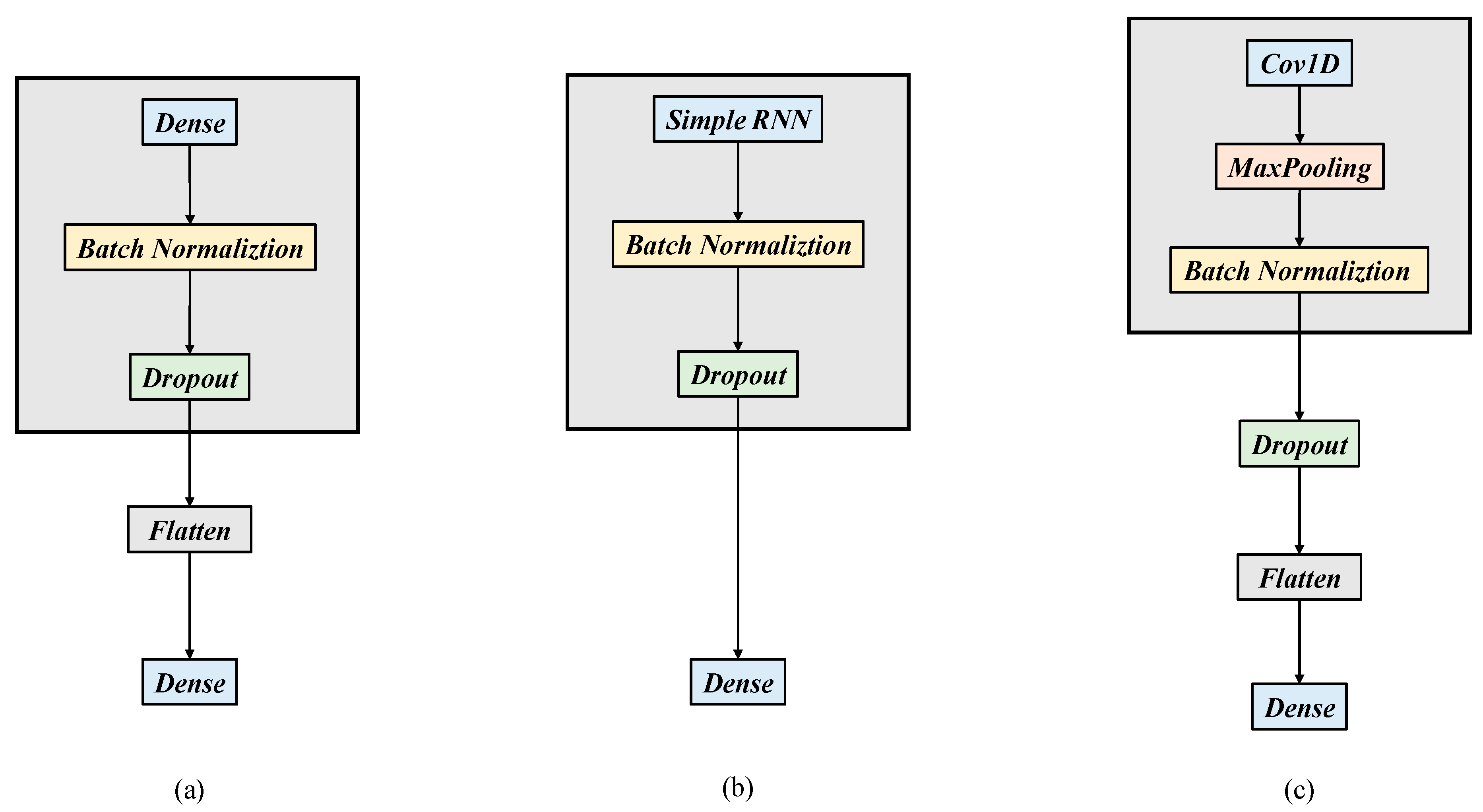
The various architectures of the neural network are shown in Figure 3. Part of the figure only shows one layer of the architecture of each deep learning network. But, we actually conducted experiments using one- and three-layer stacking architectures. At the output layer, it is worth noting that we will use excitation functions for the classification tasks, binary classification will use Sigmoid, and multivariate classification will use Softmax. We will describe the detailed parameter quantities of each neural network in the following sections.

3.1.1. DNN

The architecture of DNN is shown in Figure 3a, which mainly consists of the input Dense layer, Batch Normalization (BN) layer, Dropout layer, Flatten layer, and output Dense layer. The number of parameters in each layer and the corresponding number of nodes are shown in Table 5. In order to reduce the occurrence of overfitting, we add a BN layer and a Dropout layer to each layer, normalize each batch during the training process, and the Dropout layer randomly discards neurons at a certain proportion in each layer. Both effectively prevent neurons from becoming overly dependent on certain features.

3.1.2. RNN

The architecture of RNN is shown in Figure 3b. Similar to DNN, it also consists of a Simple RNN, BN layer, and Dropout layer. But, there is no Flatten layer in RNN. This is because, in RNN, the input can be a sequence, such as a text sentence or a time series, and the RNN layer is designed to be able to process sequence data. Therefore, there is no need to add a Flatten layer to convert the dimensions of the data. The number of parameters in each layer and the corresponding number of nodes are shown in Table 6.

3.1.3. CNN

The architecture of CNN is shown in Figure 3c, which mainly consists of Conv1D and MaxPooling layers. Unlike DNN and RNN where each hidden layer contains a BN layer and Dropout layer, CNN only introduces a BN layer and Dropout layer before the output layer. This design choice is attributed to the effectiveness of MaxPooling layers 1 and 2 in preventing overfitting. These layers facilitate feature extraction after convolution, emphasizing key data and minimizing irrelevant noise. Table 7 outlines the details of the number of parameters per layer and the corresponding number of nodes of CNN.

3.1.4. LSTM

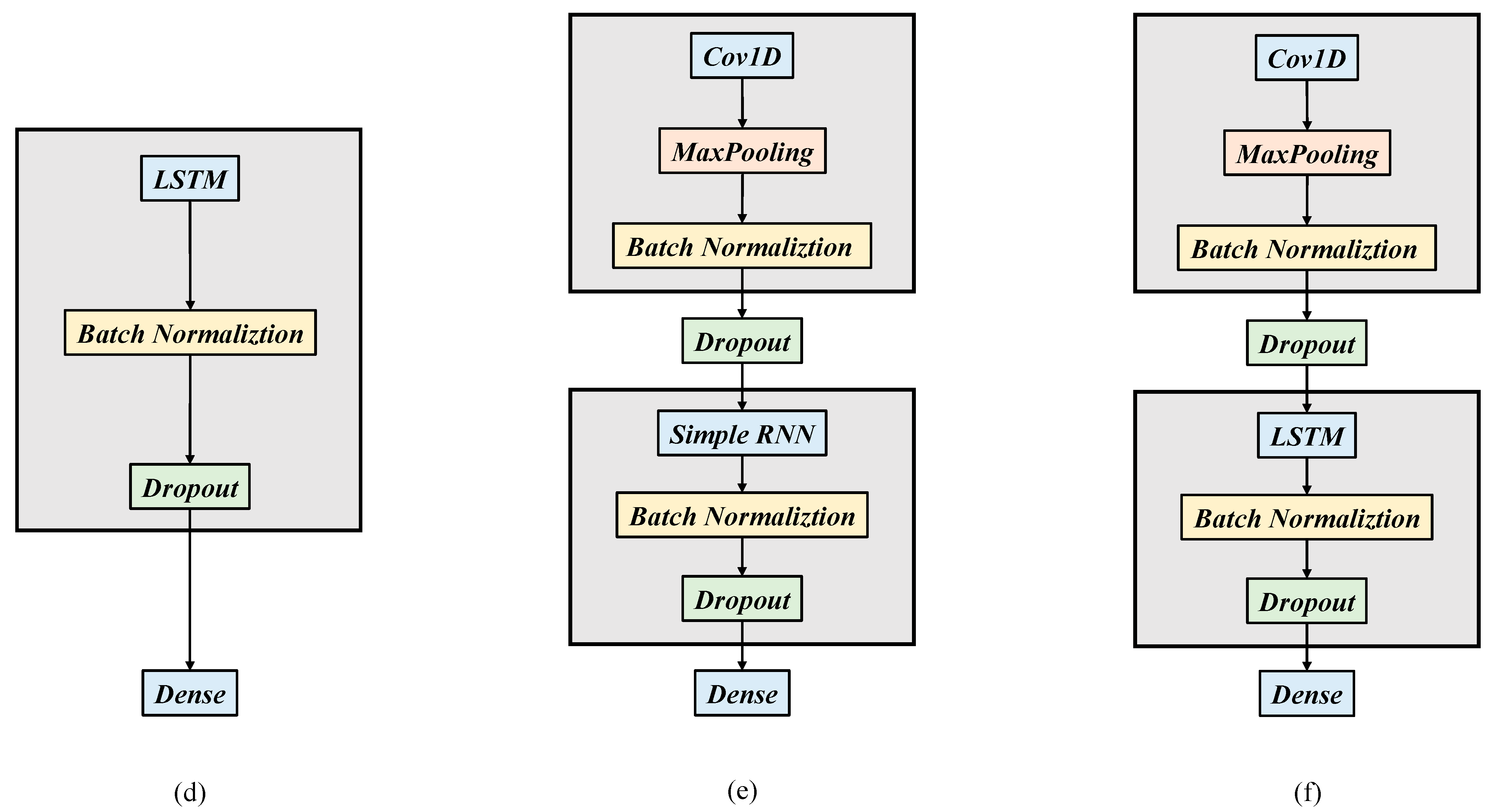
The architecture of LSTM is shown in Figure 3d. LSTM is a variant of RNN designed to better handle long sequence dependencies and overcome the vanishing gradient problem of traditional RNN. The number of parameters in each layer and the corresponding number of nodes are shown in Table 7. The architecture of CNN + RNN is shown in Figure 3e. In this architecture, there are two architectures: one with one convolutional layer and one recurrent layer, and one with three convolutional layers and three recurrent layers. The number of parameters in each layer and the corresponding number of nodes are shown in Table 8.

3.1.5. CNN + RNN

The architecture of CNN + RNN is shown in Figure 3e. In this architecture, there are two architectures: one with one convolutional layer and one recurrent layer, and one with three convolutional layers and three recurrent layers. The number of parameters in each layer and the corresponding number of nodes are shown in Table 9.

3.1.6. CNN + LSTM

The architecture of CNN + RNN is shown in Figure 3f. In this architecture, there are two architectures: one with one convolutional layer and one recurrent layer, and one with three convolutional layers and three recurrent layers. The number of parameters in each layer and the corresponding number of nodes are shown in Table 10.

3.2. Transformer

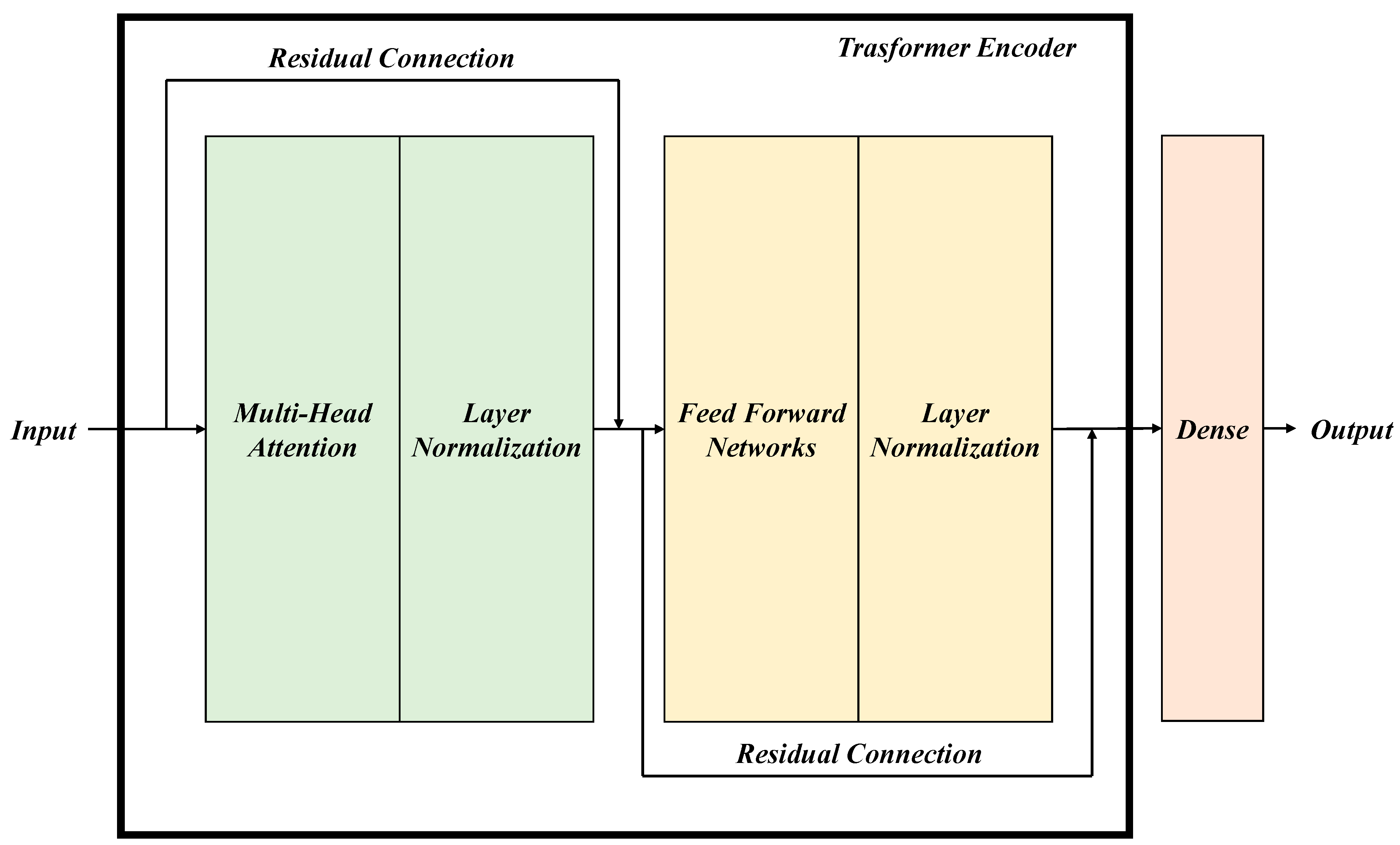
The architecture of the Transformer used in this paper is shown in Figure 4, and the detailed parameters are shown in Table 11. The main architecture of Transformer includes an encoder and a decoder, but for binary and multivariate classification tasks involving a single output sequence, the decoder is unnecessary. Therefore, only encoders [7] are used in our architecture.
Additionally, two structures can be omitted for classification purposes. First, word embedding, which converts language vocabulary into a vector space for deep learning analysis, is unnecessary for our model. The material we are classifying is already in numeric form and converted to integers, thus eliminating the need for word embeddings. Secondly, positional encoding (Positional Encoding) used to determine the relative and absolute positions of tokens in sentences is not needed for our dataset. The length and composition of similar “sentences” in our data are fixed, making this structure not necessary [5].

3.2.1. Self Attention

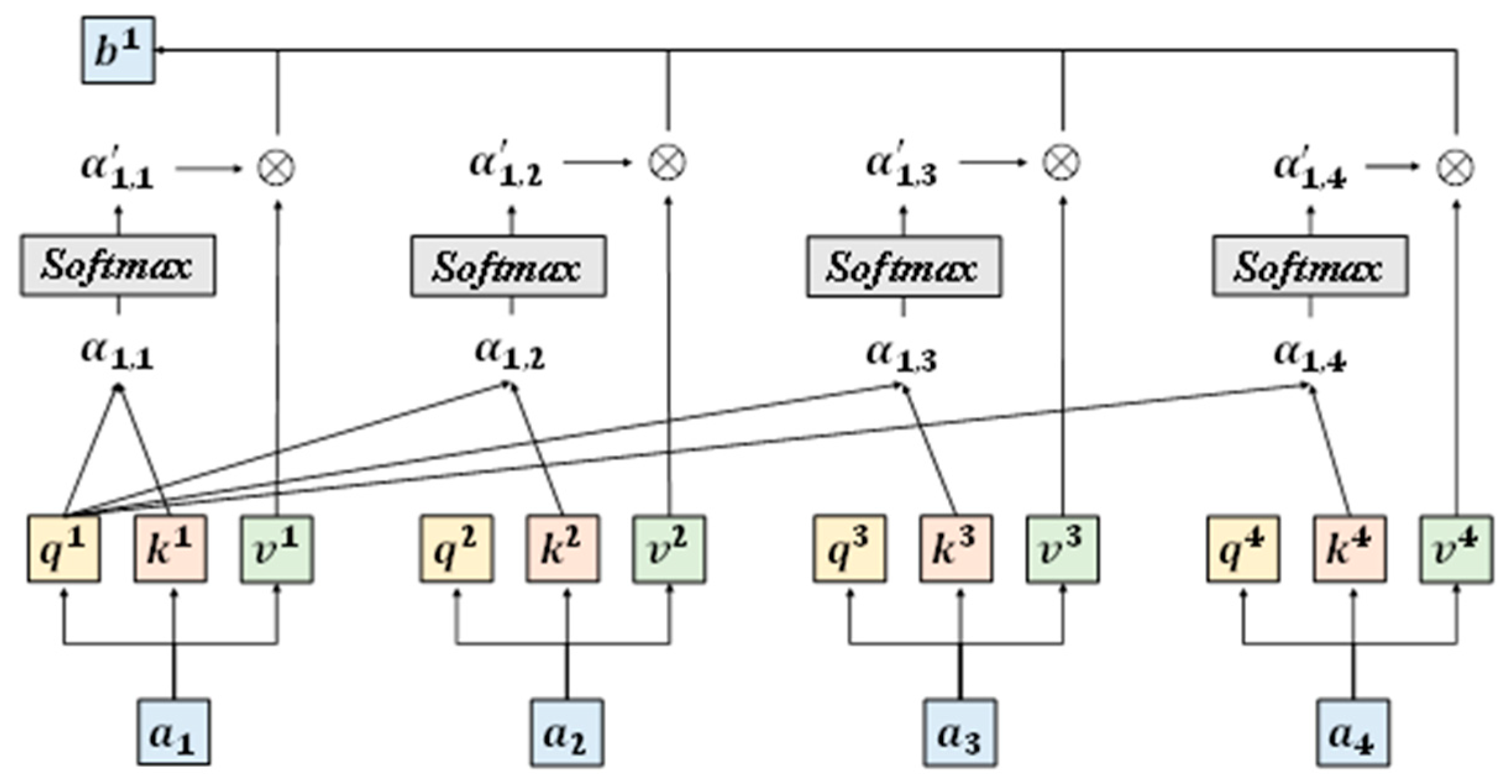
The most important structures in Transformer are the self-attention mechanism and the multi-head attention mechanism. The schematic diagram of finding one of the outputs b 1 is shown in Figure 5.
First, we assume that the input is a sequence of four vectors a 1 , a 2 , a 3 , a 4 , and then multiply these four vectors by three transformation matrices W Q ,   W K and W V to get each q i , k i and v i corresponding to each input vector, that is:
q i = W Q a i
k i = W k a i
v i = W v a i
where   i = 1 ,   2 ,   3 ,   4 .
After getting these three elements, we can start attention, as shown in Figure 5. Here, we take the output b 1 as an example.
First, we perform Scaled Dot Product on q 1 with k 1 , k 2 , k 3 and k 4 , and we can get α 1 , 1 , α 1 , 2 ,   α 1 , 3 and α 1 , 4 .
Then, we perform Softmax on α 1 , 1 ,     α 1 , 2 , α 1 , 3 and α 1 , 4 , we can get α 1 , 1 ,   α 1 , 2 , α 1 , 3 and α 1 , 4 , and then α 1 , 1 ,     α 1 , 2 .
α 1 , 1 = q 1 k 1
α 1 , 2 = q 1 k 2
α 1 , 3 = q 1 k 3
α 1 , 4 = q 1 k 4
α 1 , 3 and α 1 , 4 are multiplied by v 1 , v 2 ,     v 3 and v 4 , respectively, and finally the four results are added to obtain the output b 1 , that is:
b 1 = i = 1 4 α 1 , i v i = i = 1 4 Softmax α 1 , i v i
As for b 2 , b 3 and b 4 , we can refer to Formula (8) and express it as the following formula:
b 2 = i = 1 4 α 2 , i v i
b 3 = i = 1 4 α 3 , i v i
b 4 = i = 1 4 α 4 , i v i

3.2.2. Multi-Head Attention

There is an advanced version of self-attention called the multi-head attention mechanism. In the previous chapter, the input was multiplied only once by the transformation matrices W Q ,   W K , and W v , and then its corresponding q   , k   , and v   values.
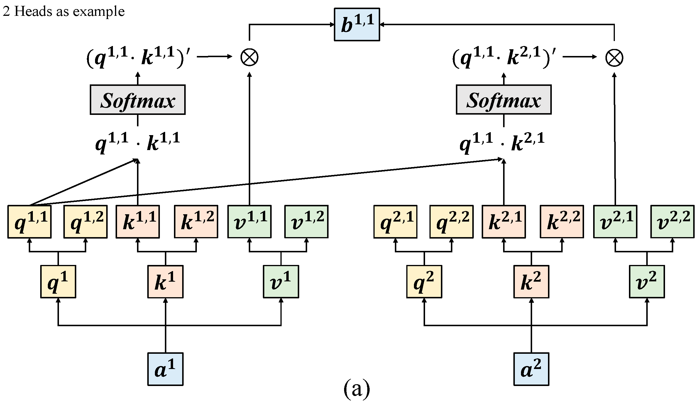
In the multi-head attention mechanism, taking two inputs a 1 and a 2 as an example, q , k , and v will be multiplied again by a transformation matrix. Assuming there are two attention heads, two types of q , k , and v will be obtained, respectively. As shown in Figure 6a, the first attention head q 1 , 1 will perform an attention calculation with k 1 , 1 , then it will perform Softmax, and then it will multiply by v 1 , 1 . Next, q 1 , 1 will be calculated with k 2 , 1 for attention, then Softmax, and finally multiplied by v 2 , 1 . Finally, adding the previous two results gives b 1 , 1 , that is:
b 1 , 1 = i = 1 n Softmax q 1 , 1 k n , 1 v n , 1
where n is 2, which is the number of heads.
Then, as shown in Figure 6b, the second attention head q 1 , 2 will perform an attention calculation with k 1 , 2 , then it will perform Softmax, and finally it will multiply by v 1 , 2 . Then, q 1 , 2 performs an attention calculation with k 2 , 2 , then it performs Softmax, and finally it multiplies v 2 , 2 . Finally, adding the previous two results gives b 1 , 2 , that is:
b 1 , 2 = i = 1 n Softmax q 1 , 2 k n , 1 v n , 1
Finally, these two outputs are concatenated and multiplied by an output transformation matrix W O to obtain the final output b 1 , as shown in Figure 6c.

3.2.3. Feed Forward Network

In our architecture, the main classification task is performed in a feed forward network. The feed forward network lies behind the multi-head attention mechanism and consists of two fully connected layers. The activation function of the first layer is Relu, and no activation function is used in the second layer.

3.2.4. Layer Normalization

Layer Normalization is a technique that normalizes each input feature independently, aiming to eliminate scale differences between different features and maintain output stability. Layer normalization helps control the output of each layer to keep it within a smaller range, helping to prevent gradient explosion. Sometimes, it can accelerate the convergence of the model and improve the training speed. Compared with Batch Normalization, Layer Normalization does not need to consider batch information.

3.2.5. Residual Connection

In neural networks, complex features are learned by stacking multiple layers. However, as the number of network layers increases, the gradient may gradually decrease, making the training process difficult. The idea of residual connections is to introduce skip connections, allowing the network to directly skip one or more layers and add the input signal to the output signal. In this way, even in deep networks, the information of the original input signal can still be propagated directly to deeper layers, thus helping to alleviate the vanishing gradient problem.

4. Experimental Results

4.1. Experimental Environment

The equipment specifications and environment settings used in this article are shown in Table 12. Since simply using tensorflow will cause the training speed to be too slow; this article chooses to use tensorflow-gpu to run our model to speed up the training. The hyperparameters of the six neural network models are shown in Table 13. Due to the large size of the dataset, we increased the batch size to 1024.

4.2. Experimental Metrics

We employ four metrics to evaluate the model’s predictions of the number of accurate and inaccurate outcomes. These metrics are as follows: (1) True Positives (TPs), which represent the number of correctly classified benign samples; (2) False Positives (FPs), which represent the number of attack samples that are incorrectly predicted to be benign; (3) True Negatives (TNs), which represent the correct number of classified attack samples; and (4) False Negatives (FNs), indicating the number of benign samples that are incorrectly predicted as attacks. These four metrics produce four evaluation metrics: accuracy, precision, recall, and F1-Score. Accuracy measures the proportion of correctly classified samples. Precision measures the accuracy of predicting benign samples, while recall measures the accuracy of identifying benign samples. The F1-Score is an indicator of the classification model’s performance and is the harmonic mean of precision and recall. The formulas for these metrics are summarized below:
A c c u r a c y = T P + T N T P + T N + F P + F N
P r e c i s i o n = T P T P + F P
R e c a l l = T P T P + F N
F 1 - S c o r e = 2 × P r e c i s i o n × R e c a l l P r e c i s i o n + R e c a l l

4.3. Experimental Result

The accuracy results of DNN are shown in Table 14, and the evaluation results of DNN are shown in Table 15.
The accuracy results of RNN are shown in Table 16, and the evaluation results of RNN are shown in Table 17.
The accuracy results of CNN are shown in Table 18, and the evaluation results of CNN are shown in Table 19.
The accuracy results of LSTM are shown in Table 20, and the evaluation results of LSTMare shown in Table 21.
The accuracy results of CNN + RNN are shown in Table 22, and its evaluation results are shown in Table 23.
The accuracy results of CNN + LSTM are shown in Table 24, and its evaluation results are shown in Table 25.
The accuracy results of Transformer are shown in Table 26 and its evaluation results are shown in Table 27 and Table 28.

4.4. Accuracy Figure

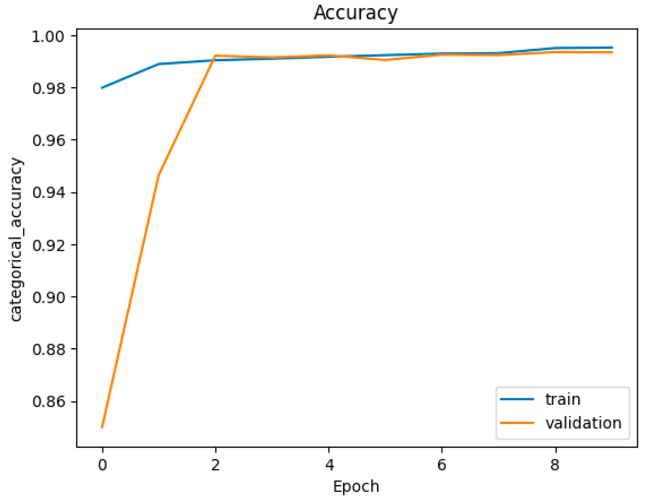
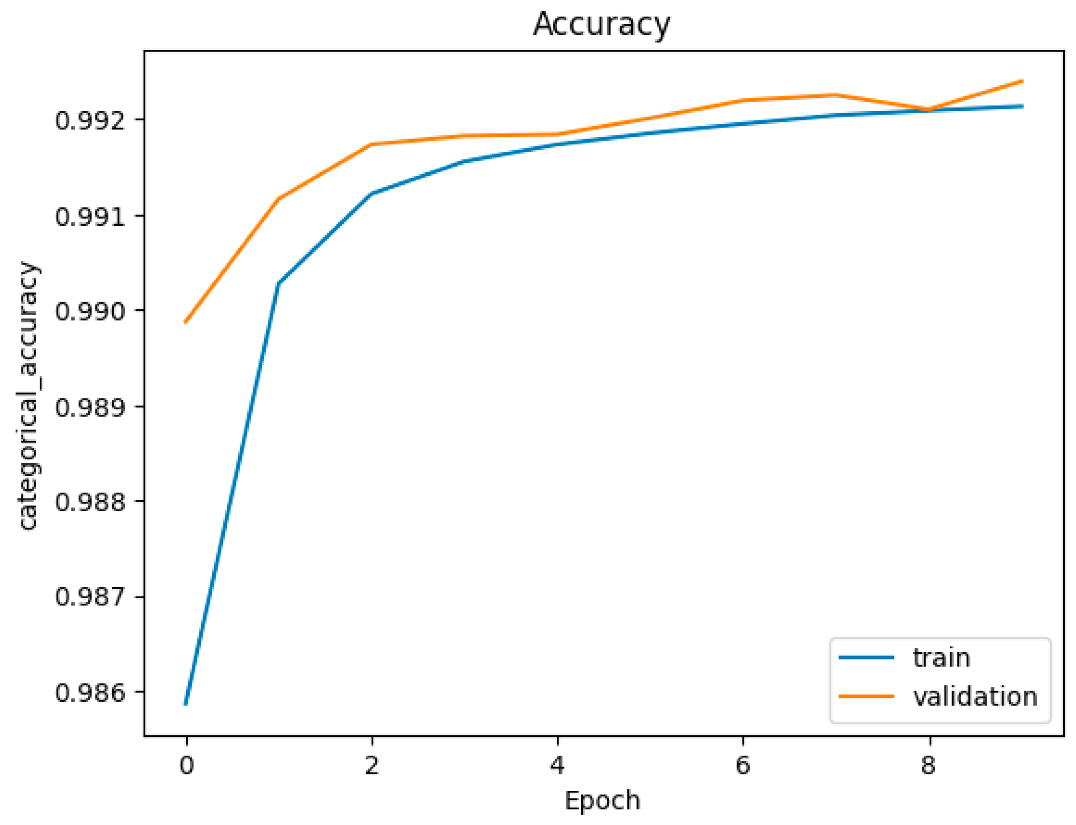
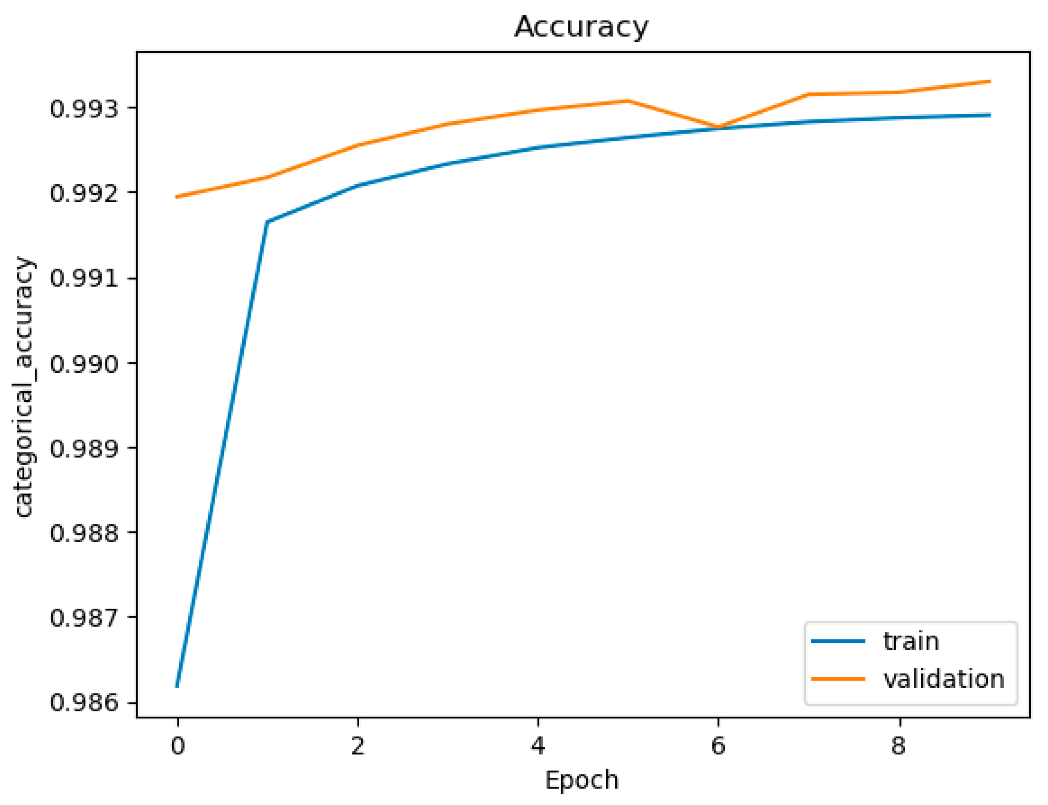
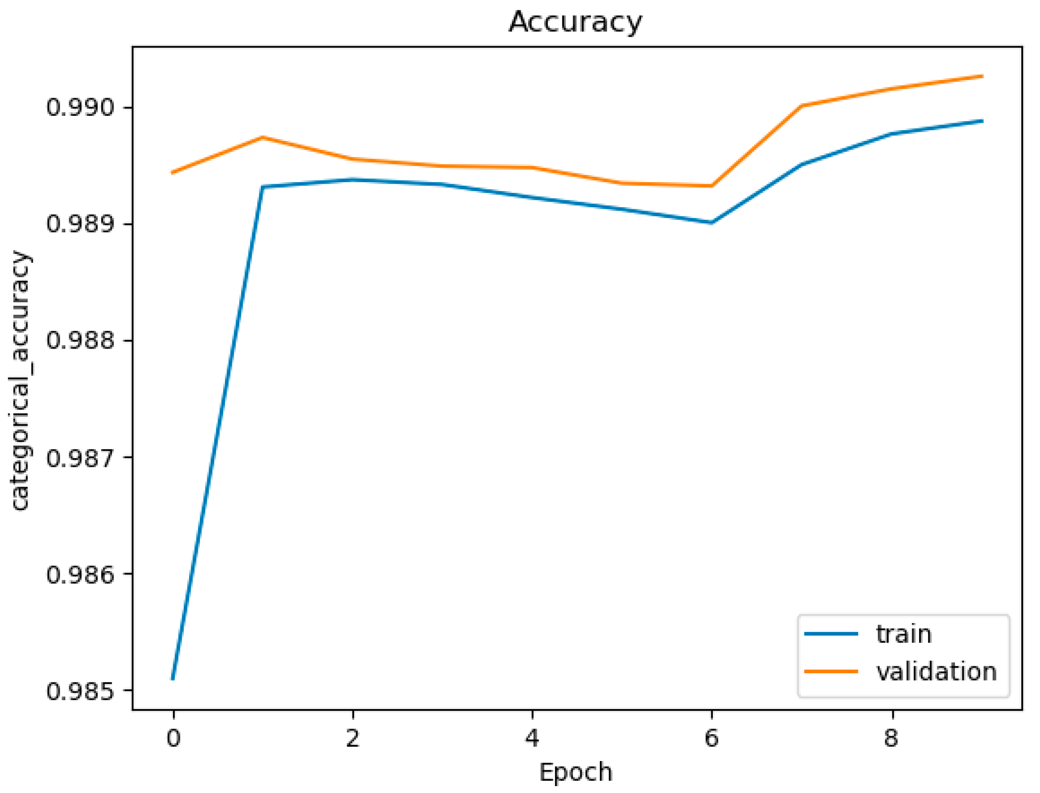
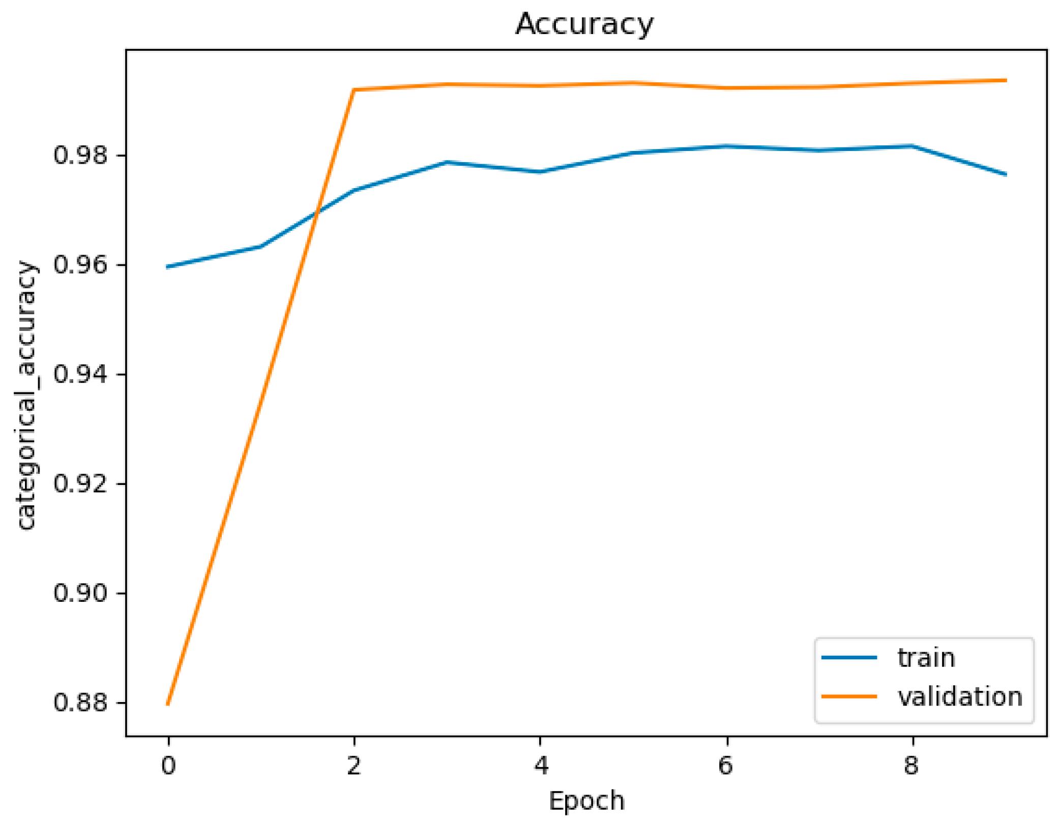
In this subsection, we show the comparison between the validation and training accuracy in every model. In Figure 7, Figure 8, Figure 9, Figure 10, Figure 11, Figure 12 and Figure 13, we provide the most complex case for each model (DNN, RNN, CNN, LSTM, CNN + RNN, CNN + LSTM, Transformer, etc.). As shown in Figure 7, Figure 8, Figure 9, Figure 10, Figure 11, Figure 12 and Figure 13, there is no overfitting.

4.5. Time Consumption

The time consumption of each model is show in Table 29.

4.6. Confusion Matrices

In this subsection, we show the confusion matrix in every model. In Table 30, Table 31, Table 32, Table 33, Table 34, Table 35 and Table 36 we provide the most complex case for each model (DNN, RNN, CNN, LSTM, CNN + RNN, CNN + LSTM, Transformer, etc.).

5. Conclusions

This research is based on the CIC-IoT-2023 dataset and conducts an in-depth discussion and analysis of IoT network intrusion detection. We apply deep learning methods to improve the detection performance of abnormal behaviors and intrusions. Compared with other papers, we further use the Transformer model and further use multi-class classification. The experimental results show that in binary classification, DNN and CNN + LSTM have the highest accuracy, while in multi-class classification, the Transformer model has the highest accuracy. This proves the potential application value of deep learning methods in IoT network intrusion detection. In the future, the dataset can be reconstructed and balanced to avoid the unpredictable situation of minority category attacks, so that these 34 categories can be directly used for classification to improve the generalization ability of the model and remove some features that have no impact on model classification to improve classification efficiency.
The method used in this study brings new possibilities to the field of IoT network intrusion detection. It is hoped that the results of this study can provide a valuable reference for the development of the field of IoT security.

Author Contributions

Conceptualization, S.-M.T. and Y.-C.W.; methodology, S.-M.T. and Y.-C.W.; software and data curation, Y.-Q.W.; funding acquisition, S.-M.T. All authors have read and agreed to the published version of the manuscript.

Funding

This research was funded by National Science and Technology Council, Taiwan grant number NSTC 112-2221-E-027-079-MY2.

Data Availability Statement

The data can be shared up on request. The data are not publicly available due to privacy restrictions.

Conflicts of Interest

The authors declare no conflict of interest.

References

  1. Abbas, S.; Al Hejaili, A.; Sampedro, G.A.; Abisado, M.A.; Almadhor, A.M.; Shahzad, T.; Ouahada, K. A novel federated edge learning approach for detecting cyberattacks in IoT infrastructures. IEEE Access 2023, 11, 112189–112198. [Google Scholar] [CrossRef]
  2. Asharf, J.; Moustafa, N.; Khurshid, H.; Debie, E.; Haider, W.; Wahab, A. A review of intrusion detection systems using machine and deep learning in Internet of Things: Challenges solutions and future directions. Electronics 2020, 9, 1177. [Google Scholar] [CrossRef]
  3. Dadkhah, S.; Mahdikhani, H.; Danso, P.K.; Zohourian, A.; Truong, K.A.; Ghorbani, A.A. Towards the development of a realistic multidimensional IoT pofiling dataset. In Proceedings of the 2022 19th Annual International Conference on Privacy, Security & Trust (PST), Fredericton, NB, Canada, 22–24 August 2022; pp. 1–11. [Google Scholar]
  4. Talpur, A.; Gurusamy, M. Machine learning for security in vehicular networks: A comprehensive survey. IEEE Commun. Surv. Tutor. 2022, 24, 346–379. [Google Scholar] [CrossRef]
  5. Li, Q.F.; Liu, Y.Q.; Niu, T.; Wang, X.M. Improved Resnet Model Based on Positive Traffic Flow for IoT Anomalous Traffic Detection. Electronics 2023, 12, 3830. [Google Scholar] [CrossRef]
  6. Wang, Y.C.; Yng, Y.C.; Chen, H.X.; Tseng, S.M. Network anomaly intrusion detection based on deep learning approach. Sensors 2023, 23, 2171. [Google Scholar] [CrossRef] [PubMed]
  7. Ahmed, S.W.; Kientz, F.; Kashef, R. A modified transformer neural network (MTNN) for robust intrusion detection in IoT networks. In Proceedings of the 2023 International Telecommunications Conference (ITC-Egypt), Alexandria, Egypt, 18–20 July 2023; pp. 663–668. [Google Scholar]
  8. Mezina, A.; Burget, R.; Travieso-González, C.M. Network Anomaly Detection with Temporal Convolutional Network and U-Net model. IEEE Access 2021, 9, 143608–143622. [Google Scholar] [CrossRef]
  9. He, M.S.; Wang, X.J.; Wei, P.; Yang, L.; Teng, Y.L.; Lyu, R.J. Reinforcement learning meets network intrusion detection: A transferable and adaptable framework for anomaly behavior identification. IEEE Trans. Netw. Serv. Manag. 2024, 21, 2477–2492. [Google Scholar] [CrossRef]
  10. Jony, A.I.; Arnob, A.K.B. A long short-term memory based approach for detecting cyber attacks in IoT using CIC-IoT2023 dataset. J. Edge Comput. 2024, 3, 28–42. [Google Scholar] [CrossRef]
  11. Jaradat, A.S.; Nasayreh, A.; Al-Na’amneh, Q.; Gharaibeh, H.; Al Mamlook, R.E. Genetic optimization techniques for enhancing web attacks classification in machine learning. In Proceedings of the IEEE International Conference on 11 Dependable 2023, Autonomic & Secure Computing, Abu Dhabi, United Arab Emirates, 14–17 November 2023; pp. 0130–0136. [Google Scholar]
  12. Guo, G.; Pan, X.; Liu, H.; Li, F.; Pei, L.; Hu, K. An IoT intrusion detection system based on TON IoT network dataset. In Proceedings of the 2023 IEEE 13th Annual Computing and Communication Workshop and Conference (CCWC), Las Vegas, NV, USA, 8–11 March 2023; pp. 0333–0338. [Google Scholar]
  13. Neto, E.C.P.; Dadkhah, S.; Ferreira, R.; Zohourian, A.; Lu, R.; Ghorbani, A.A. CICIoT2023: A real-time dataset and benchmark for large-scale attacks in IoT environment. Sensors 2023, 23, 5941. [Google Scholar] [CrossRef]
  14. Shtayat, M.M.; Hasan, M.K.; Sulaiman, R.; Islam, S.; Khan, A.U.R. An explainable ensemble deep learning approach for intrusion detection in industrial Internet of Things. IEEE Access 2023, 11, 115047–115061. [Google Scholar] [CrossRef]
  15. Vaswani, A.; Shazeer, N.; Parmar, N.; Uszkoreit, J.; Jones, L.; Gomez, A.N.; Kaiser, L.; Polosukhin, I. Attention is all you need. In Advances in Neural Information Processing Systems; MIT Press: Cambridge, MA, USA, 2023; Volume 30. [Google Scholar]
  16. Haque, S.; EI-Moussa, F.; Komninos, N.; Muttukrishnan, R. A systematic review of data-driven attack detection trends in IoT. Sensors 2023, 23, 7191. [Google Scholar] [CrossRef] [PubMed]
  17. Le, T.T.H.; Wardhani, R.W.; Putranto, D.S.C.; Jo, U.; Kim, H. Toward enhanced attack detection and explanation in intrusion detection system-based IoT environment data. IEEE Access 2023, 11, 131661–131676. [Google Scholar] [CrossRef]
Figure 1. Architecture diagram of this paper.
Futureinternet 16 00284 g001
Figure 2. Distribution of converted labels containing benign traffic.
Futureinternet 16 00284 g002
Figure 3. (a) Architecture diagram of DNN, (b) architecture diagram of RNN, (c) architecture diagram of CNN, (d) architecture diagram of LSTM, (e) architecture diagram of CNN + RNN, and (f) architecture diagram of CNN + LSTM.
Futureinternet 16 00284 g003aFutureinternet 16 00284 g003b
Figure 4. Transformer encoder architecture diagram.
Futureinternet 16 00284 g004
Figure 5. The schematic diagram of finding one of the outputs b 1 .
Futureinternet 16 00284 g005
Figure 6. (a) The schematic diagram of finding one of the output b 1 , 1 ; (b) the schematic diagram of finding one of the output b 1 , 2 ; and (c) the schematic diagram of adding two results.
Futureinternet 16 00284 g006aFutureinternet 16 00284 g006b
Figure 7. Accuracy figure of DNN with (layer = 3, Node = 768, multi-class).
Futureinternet 16 00284 g007
Figure 8. Accuracy figure of RNN (with layer = 3, node = 768, multi-class classification).
Futureinternet 16 00284 g008
Figure 9. Accuracy figure of CNN (with layer = 3, node = 768, multi-class classification).
Futureinternet 16 00284 g009
Figure 10. Accuracy figure of LSTM (with layer = 3, node = 768, multi-class classification).
Futureinternet 16 00284 g010
Figure 11. Accuracy figure of CNN + RNN (with layer = 3, node = 768, multi-class classification).
Futureinternet 16 00284 g011
Figure 12. Accuracy figure of CNN + LSTM (with layer = 3, node = 768, multi-class classification).
Futureinternet 16 00284 g012
Figure 13. Accuracy figure of Transformer (with Dense Dimension = 2048, Number of Heads = 1, Number of Layers = 1, multi-class classification).
Futureinternet 16 00284 g013
Table 1. Related works/baseline schemes.
PaperDatasetClassificationDL MethodAccuracyInference Time 1
[1]CIC-IoT-2023BinaryDNN based on Federated Learning99.00%
[6]CIC-IDS-2018Binary, Multi-classDNN, RNN, CNN, LSTM,
CNN + LSTM, and CNN + RNN
98.85%Multi-Class:
LSTM: 3.451 (ms)
CNN + LSTM: 4.31 (ms)
[7]ToN-IoTBinaryLSTM, RNN, and Transformer87.79%Binary Class
LSTM: 27 (s)
RNN: 35 (s)
[9]CIC-IoT-2023Multi-classDeep Reinforcement Learning95.60%
[10]CIC-IoT-2023Multi-classLTSM98.75%
[11]CIC-IoT-2023Not MentionedGradient Boost, MLP,
Logistic Regression, and KNN
95.00%
[13]CIC-IoT-2023Binary, Multi-classDNN99.44%, 99.11%
[8]KD999Multi-classCNN, Autoencoder, FCN
RNN, U-Net, TCN, and TCN + LSTM
97.7%Multi-Class
CNN: 5 (min/epoch)
TCN + LSTM: 11 (min/epoch)
1 Inference time is copy from references.
Table 2. The number of each label containing benign traffic.
LabelQuantitysLabelQuantitysLabelQuantitys
DDoS-ICMP_Flood7,200,504Mirai-greeth_flood991,866DoS-HTTP_Flood71,864
DDoS-UDP_Flood5,412,287Mirai-udpplain890,576Vulnerability Scan37,382
DDoS-TCP_Flood4,497,667Mirai-greip_flood751,682DDoS-SlowLoris23,246
DDoS-PSHACK_Flood4,094,755DDoS-ICMP_Fragmentation452,489DictionaryBruteForce13,064
DDoS-SYN_Flood4,059,190MITM-ArpSpoofing307,593BrowserHijacking5859
DDoS-RSTFINFlood4,045,190DDoS-UDP_Fragmentation286,925CommandInjection5409
DDoS-SynonymousIP_Flood3,598,138DDoS-ACK_Fragmentation285,104SQL Injection5245
DoS-UDP_Flood3,318,595Recon-HostDiscovery178,911XSS3946
DoS-TCP_Flood2,671,445Recon-OSScan134,378Backdoor_Malware3218
DoS-SYN_Flood2,028,834Recon-PortScan98,259Recon-PingSweep2262
Benign1,098,195DDoS-HTTP_Flood71,864Uploading_Attack1252
Table 3. The features used in CIC-IoT-2023.
FeatureName
1Flow duration
2Header Length
3Protocol
4Type
5Duration
6Rate Mrate Drate
7fin flag number
8syn flag number
9rst flag number
10psh flag number
11ack flag number
12ece flag number
13cwr flag number
14ack count
15syn count
16fin count
17urg count
18rst count
19HTTP
20HTTPS
21DNS
22Telnet
23SMTP
24SSH
25IRC
26TCP
27UDP
28DHCP
29ARP
30ICMP
31IPv
32LLC
33Tot sum
34Min
35Max
36AVG
37Std
38Tot size
39IAT
40Number
41Magnitude
42Radius
43Covariance
44Variance
45Weight
46Flow duration
Table 4. The number of neurons and units of each of the neural networks.
LayersNeuronsUnits
1256256
512512
768768
325664 + 64 + 128
512128 + 128 + 256
768256 + 256 + 256
Table 5. Number of parameters and nodes of DNN.
LayersNeuronsParameters
BinaryMulti-Class
125613,31315,112
51226,62530,216
76839,93745,320
325619,52119,976
51263,61764,520
768146,945148,744
Table 6. Number of parameters and nodes of RNN.
LayersNeuronsParameters
BinaryMulti-Class
125678,84980,648
512288,769292,360
768629,761635,144
325644,09744,552
512161,921162,824
768343,553345,352
Table 7. Number of parameters and nodes of CNN.
LayersNeuronsParameters
BinaryMulti-Class
125613,31315,112
51226,62530,216
76839,93745,320
325619,52119,976
51263,61764,520
768146,945148,744
Table 8. Number of parameters and nodes of LSTM.
LayersNeuronsParameters
BinaryMulti-Class
1256311,553313,352
5121,147,3931,150,984
7682,507,5212,512,904
3256173,121173,576
512354,433619,528
7681,364,2251,366,024
Table 9. Number of parameters and nodes of CNN + RNN.
LayersNeuronsParameters
BinaryMulti-Class
125678,849133,160
512288,769365,864
768629,761729,640
325644,09786,568
512161,921215,336
768343,553397,864
Table 10. Number of parameters and nodes of CNN + LSTM.
LayersNeuronsParameters
BinaryMulti-Class
1256420,041428,840
5121,346,8491,350,440
7682,790,9452,796,328
3256246,625247,080
512756,641757,544
7681,479,7131,481,512
Table 11. Number of parameters of Transformer.
Dense Dimension
(FFN)
Number of HeadsNumber of Layers
(Encoder)
Parameters
BinaryMulti-Class
2561132,73333,062
128 20,82921,158
512 56,54156,870
1024 104,157104,486
2048 199,389199,718
2 41,33541,664
4 58,53958,868
8 94,94793,276
241,38141,710
458,67759,006
894,26993,598
Table 12. Number of parameters of Transformer.
ProjectProperties
OSWindows 11
CPUIntel® Core™ i7-13700 Processor
GPUNVIDA Geforce RTX 4080
Memory128 GB
Disk1TB SSD
Python3.7.16
NVIDIA CUDA11.3.1
FrameworkTensorflow-gpu 2.5 & 2.6
Table 13. Number of parameters of Transformer.
HyperparameterValue
Batch Size1024
Epochs10
Learning Rate0.001
Dropout0.1
Table 14. The accuracy results of DNN.
LayersNeuronsAccuracy (%)
BinaryMulti-Class
125699.4897.35
51299.4797.73
76899.5399.13
325699.5699.16
51299.5699.23
76899.5699.36
Table 15. The evaluation results of DNN.
LayerNodePrecision (%)Recall (%)F1-Score (%)
BinaryMulti-ClassBinaryMulti-ClassBinaryMulti-Class
125699.5197.3599.4897.3599.4997.30
51299.5197.7499.4897.7399.4997.66
76899.4999.1299.4799.1399.4899.10
325699.5499.1799.5399.1699.5499.12
51299.5799.2499.5699.2399.5699.18
76899.5799.3599.5699.3699.5799.32
Table 16. The accuracy results of RNN.
LayersNeuronsAccuracy (%)
BinaryMulti-Class
125699.4999.21
51299.4999.22
76899.4899.24
325699.5399.26
51299.5099.27
76899.5099.28
Table 17. The evaluation results of RNN.
LayerNodePrecision (%)Recall (%)F1-Score (%)
BinaryMulti-ClassBinaryMulti-ClassBinaryMulti-Class
125699.5199.2199.4999.2199.5099.17
51299.5099.2399.4999.2299.4999.19
76899.5199.2399.4899.2499.4999.21
325699.5499.2699.5399.2699.5399.21
51299.5099.2799.5099.2799.5099.24
76899.5299.2899.5099.2899.5199.23
Table 18. The evaluation results of CNN.
LayerNodePrecision (%)Recall (%)F1-Score (%)
BinaryMulti-ClassBinaryMulti-ClassBinaryMulti-Class
125699.5199.2199.4999.2199.5099.17
51299.5099.2399.4999.2299.4999.19
76899.5199.2399.4899.2499.4999.21
325699.5499.2699.5399.2699.5399.21
51299.5099.2799.5099.2799.5099.24
76899.5299.2899.5099.2899.5199.23
Table 19. The evaluation results of CNN.
LayerNodePrecision (%)Recall (%)F1-Score (%)
BinaryMulti-ClassBinaryMulti-ClassBinaryMulti-Class
125699.3096.1199.2796.0699.2895.93
51299.2997.8399.2797.7399.2897.64
76899.3191.9599.2490.9199.2789.88
325699.5099.1899.4899.1999.4899.15
51299.5199.2199.4899.2399.4999.1
76899.5299.2399.4899.2599.5099.21
Table 20. The accuracy results of LSTM.
LayersNeuronsAccuracy (%)
BinaryMulti-Class
125699.5199.28
51299.5199.28
76899.5099.28
325699.5499.32
51299.5499.21
76899.5299.34
Table 21. The evaluation results of LSTM.
LayerNodePrecision (%)Recall (%)F1-Score (%)
BinaryMulti-ClassBinaryMulti-ClassBinaryMulti-Class
125699.5299.2799.5199.2899.5199.24
51299.5399.2899.5199.2899.5299.25
76899.5399.2899.5099.2899.5199.24
325699.5599.3199.5499.3299.5499.28
51299.5599.3199.5499.3199.5499.28
76899.5499.3299.5499.3499.5299.31
Table 22. The accuracy results of CNN + RNN.
LayersNeuronsAccuracy (%)
BinaryMulti-Class
125699.3799.15
51299.2999.19
76899.4599.11
325699.4699.16
51299.4299.07
76899.1599.03
Table 23. The evaluation results of CNN + RNN.
LayerNodePrecision (%)Recall (%)F1-Score (%)
BinaryMulti-ClassBinaryMulti-ClassBinaryMulti-Class
125699.4499.1599.3799.1599.3999.10
51299.3699.1999.2999.1999.3299.15
76899.4899.1299.4599.1199.4799.04
325699.4899.1599.4699.1699.4799.12
51299.4399.0799.4299.0799.4399.00
76899.2399.0299.1599.0399.1898.98
Table 24. The accuracy results of CNN + LSTM.
LayersNeuronsAccuracy (%)
BinaryMulti-Class
125699.5699.33
51299.4698.70
76899.5599.34
325699.5399.31
51299.4999.26
76899.4899.26
Table 25. The evaluation results of CNN + LSTM.
LayerNodePrecision (%)Recall (%)F1-Score (%)
BinaryMulti-ClassBinaryMulti-ClassBinaryMulti-Class
125699.5799.3199.5699.3399.5699.30
5129.5798.7099.5698.7099.5698.66
76899.5799.3399.5599.3499.5699.31
325699.5599.2999.5399.3199.5499.28
51299.4999.2599.4999.2699.4999.22
76899.4899.2599.4899.2699.4899.22
Table 26. The accuracy results of Transformer.
Dense Dimension
(FFN)
Number of HeadsNumber of Layers
(Encoder)
Accuracy (%)
BinaryMulti-Class
2561199.5199.12
128 99.5097.54
512 99.5199.40
1024 99.5199.36
2048 99.5299.21
2 99.5099.19
4 99.5098.96
8 99.5199.32
299.5099.34
499.4999.23
899.4899.24
Table 27. The precision of Transformer.
Dense Dimension
(FFN)
Number of HeadsNumber of Layers
(Encoder)
BinaryMulti-Class
2561199.5294.03
128 99.5398.72
512 99.5299.27
1024 99.5499.31
2048 99.5499.33
2 99.5398.88
4 99.5299.23
8 99.5395.03
299.5399.25
499.5299.32
899.4999.11
Table 28. The recall of Transformer.
Dense Dimension
(FFN)
Number of HeadsNumber of Layers
(Encoder)
BinaryMulti-Class
2561199.5093.68
128 99.5198.72
512 99.5199.27
1024 99.5299.43
2048 99.5299.33
2 99.5098.88
4 99.5094.94
8 99.5198.88
299.5099.24
499.4999.30
899.4899.11
Table 29. Time consumption of each model (per sample).
ModelBinary Testing Time (μs)Multi-Class Testing Time (μs)
DNN3.83.8
RNN77
CNN12.312.3
LSTM88
CNN + RNN1515
CNN + LSTM1818
Transformer55
Table 30. Confusion matrix figure of DNN (with layer = 3, node = 768, multi-class classification).
ActualBenign Traffic1,073,13287287800130316,6478
DDos4783,980,302271213380012149
Dos2218,8088,071,7167900347915
Recon82,7585445105220,880155013843,66415
Web-Based536707346231931212,7871
Brute Force250802193815374948520
Spoofing56,55713214113,20891945415,40525
Mirai913,504289117500182,619,129
Benign TrafficDDosDosReconWeb-BasedBrute ForceSpoofingMirai
Table 31. Confusion matrix figure of RNN (with layer = 3, node = 768, multi-class classification).
ActualBenign Traffic1,057,0737417,20440123,8660
DDos5183,980,261246311980096491
Dos2672728,083,199320046163
Recon83,296131237236,622196933,08310
Web-Based82000051752746087080
Brute Force408900383429229828122
Spoofing108,72624724,98622014352,5243
Mirai18350561100332,633,656
Benign TrafficDDosDosReconWeb-BasedBrute ForceSpoofingMirai
Predicted
Table 32. Confusion matrix figure of CNN (with layer = 3, node = 768, multi-class classification).
ActualBenign Traffic1,034,44414722,3621274741,1922
DDos8383,979,98432387640063428
Dos3662288,084,36820003749
Recon78,798209340236,72979016135,93024
Web-Based60771254852960710,2970
Brute Force356400358478240134370
Spoofing101,54123424,34988098359,6054
Mirai538063600162,633,654
Benign TrafficDDosDosReconWeb-BasedBrute ForceSpoofingMirai
Predicted
Table 33. Confusion matrix figure of LSTM (with layer = 3, node = 768, multi-class classification).
ActualBenign Traffic1,049,17916317,2452443431,4722
DDos4683,980,598240513352047136
Dos2465318,084,05428103763
Recon68,01172329247,281121217937,1282
Web-Based523010482655201692351
Brute Force3258103384142286434150
Spoofing88,611293021,8801797170373,96522
Mirai11865381900252,633,166
Benign TrafficDDosDosReconWeb-BasedBrute ForceSpoofingMirai
Predicted
Table 34. Confusion matrix figure of CNN + RNN (with layer = 3, node = 768, multi-class classification).
ActualBenign Traffic1,043,23567320,08981234,7153
DDos10883,962,688160,0783626022901768
Dos4229,6738,058,272152130471180
Recon95,6934048638217,211551436,490416
Web-Based79957058121501095131
Brute Force47721036415190427410
Spoofing131,00795027,7612030327,41523
Mirai2910,57612921130021612,620,934
Benign TrafficDDosDosReconWeb-BasedBrute ForceSpoofingMirai
Predicted
Table 35. Confusion matrix figure of CNN + LSTM (with layer = 3, node = 768, multi-class classification).
ActualBenign Traffic1,042,72031625,9293672629,1160
DDos3383,980,79426117780383258
Dos1564358,084,20710103040
Recon66,965173127251,565138615532,68947
Web-Based427361621454651084100
Brute Force3036103710177274034000
Spoofing93,7241092826,392253277363,6384
Mirai73683170001032,633,545
Benign TrafficDDosDosReconWeb-BasedBrute ForceSpoofingMirai
Predicted
Table 36. Confusion matrix figure of Transformer (with layer = 3, node = 768, multi-class classification).
ActualBenign Traffic1,050,0211264123,943611122,82866
DDos1383,975,35720313208106883262
Dos4625,2508,064,5004980060384
Recon59,53123092257,60128735,00780
Web-Based551323049607361069711
Brute Force33006025892231848481
Spoofing68,286613023,988379333392,81590
Mirai3779679212002622,625,772
Benign TrafficDDosDosReconWeb-BasedBrute ForceSpoofingMirai
Predicted
Disclaimer/Publisher’s Note: The statements, opinions and data contained in all publications are solely those of the individual author(s) and contributor(s) and not of MDPI and/or the editor(s). MDPI and/or the editor(s) disclaim responsibility for any injury to people or property resulting from any ideas, methods, instructions or products referred to in the content.