Article

Prophet–CEEMDAN–ARBiLSTM-Based Model for Short-Term Load Forecasting

1
Electric Power Science Research Institute, Yunnan Power Grid Co., Ltd., Kunming 650000, China
2
College of Electrical Engineering, Hunan University, Changsha 410000, China
*
Author to whom correspondence should be addressed.
Future Internet 2024, 16(6), 192; https://doi.org/10.3390/fi16060192
Submission received: 24 April 2024 / Revised: 13 May 2024 / Accepted: 17 May 2024 / Published: 31 May 2024

Abstract

:
Accurate short-term load forecasting (STLF) plays an essential role in sustainable energy development. Specifically, energy companies can efficiently plan and manage their generation capacity, lessening resource wastage and promoting the overall efficiency of power resource utilization. However, existing models cannot accurately capture the nonlinear features of electricity data, leading to a decline in the forecasting performance. To relieve this issue, this paper designs an innovative load forecasting method, named Prophet–CEEMDAN–ARBiLSTM, which consists of Prophet, Complete Ensemble Empirical Mode Decomposition with Adaptive Noise (CEEMDAN), and the residual Bidirectional Long Short-Term Memory (BiLSTM) network. Specifically, this paper firstly employs the Prophet method to learn cyclic and trend features from input data, aiming to discern the influence of these features on the short-term electricity load. Then, the paper adopts CEEMDAN to decompose the residual series and yield components with distinct modalities. In the end, this paper designs the advanced residual BiLSTM (ARBiLSTM) block as the input of the above extracted features to obtain the forecasting results. By conducting multiple experiments on the New England public dataset, it demonstrates that the Prophet–CEEMDAN–ARBiLSTM method can achieve better performance compared with the existing Prophet-based ones.

1. Introduction

Short-term load forecasting (STLF) is a method for predicting consumption in a particular area [1]. In the power industry, STLF has evolved into a crucial tool. With the growing use of renewable energy sources, such as hydroelectricity and wind energy, STLF has also become an important part of modern power grids [2]. Starting from power generation to distribution, all enterprises require load forecasting. The reason for this is that it helps form a sensible power generation plan [3,4].
Scholars have been performing research about short-term electricity load forecasting [5]. There are various research models for STLF, including statistical learning models, machine learning models, and deep learning models [6]. The above models have their own characteristics, but they also have limitations.
Statistical learning methods primarily utilize historical time series data for load forecasting, offering a relatively faster computational speed. Common statistical approaches include the Autoregressive Integrated Moving Average method (ARIMA) [7] and exponential smoothing (ES) [8]. ARIMA can fit stable electricity load data. However, it cannot identify unstable characteristics of electricity loads, limiting its forecasting performance. Elsaraiti et al. [9] adopted ARIMA to predict the load data for the subsequent day. The simulations show that ARIMA can predict the change trend of the electricity load. Dittmer et al. [10] adopted the ARIMA method to fit the load data of biogas plants. Goudarzi et al. [11] proposed an ensemble model incorporating ARIMA and support vector regression (SVR) to capture the relationship between input and output data. This model aims to generate accurate load-forecasted results for buildings. Jagait et al. [12] proposed an adaptive forecasting framework consisting of a Recurrent Neural Network (RNN) and ARIMA. The above method can learn the features influencing load variations from new data, producing accurate forecasted results of the electricity load in the presence of concept drift. Wang et al. [13] adopted the exponential smoothing (ES) method to forecast the electricity load of universities and improve the efficiency of power utilization.
With the development of machine learning, significant achievements have been made in the field of STLF [14,15,16,17,18].
The machine learning method has achieved a higher forecasting accuracy in STLF [14,15,16,17,18]. Machine learning models can use historical data to model the relationship between inputs and outputs [16,17,18,19]. Jiang et al. [20] employed a distribution system STLF approach, which consists of support vector regression (SVR) and a parameter optimization model for accurate STLF. Hybrid optimization involves grid traversal and particle swarm optimization. The experiment demonstrates that the above hybrid model can produce accurate forecasted results. Chen et al. [21] adopted weather data as input data for the SVR method to forecast the load for the two hours before a disaster’s occurrence. The model can improve the operational performance of smart grids and power companies, ensuring the stable operation of the smart grid. Li et al. [22] adopted the Ensemble Empirical Mode Decomposition (EMD) algorithm to decompose the input series into distinct components. The multivariate linear regression method was used to predict the low-frequency components, while a Long Short-Term Memory (LSTM) network predicted the high-frequency components. The final forecast was obtained by integrating these components. Lu et al. [23] employed Empirical Mode Decomposition (EMD) to decompose the input series into different frequency components, followed by Extreme Gradient Boosting to forecast building loads. Liu et al. [24] developed a hybrid method combining Random Forest (RF), an enhanced Sparrow Search Algorithm, and LSTM. RF was used to reduce input data dimensionality, and the improved Sparrow Search Algorithm optimized model parameters to ensure precise forecasting, predictive performance, and generalization ability.
Compared with common machine learning methods, deep neural networks have the capability to enhance the forecasting performance by learning the essential information from electricity load data through multiple layers [25,26,27,28]. Ijaz et al. [29] designed a forecasting model which consists of Artificial Neural Network (ANN) layers and Long Short-Term Memory (LSTM). Initially, the model employs an ANN layer with 11 neurons to capture the trends of the electricity load data. Subsequently, the above information is applied as the input data for the LSTM to obtain the forecasted results. Shakeel et al. [30] proposed the STLF model consisting of LightGBM and FB-Prophet. The model incorporates a location encoding layer into the FB-Prophet method, capturing the nonlinear components. Subsequently, the grid search approach is employed to tune the parameters of the LightGBM model, enhancing the forecasting performance. Chen et al. [31] used the Prophet algorithm to extract the trend information of the electricity load series. Subsequently, the LSTM method was utilized to extract the temporal features for forecasting the peak power of the distribution network. The experiments demonstrated that the forecasting performance of the Prophet–LSTM method surpassed that of the Prophet and LSTM methods. Son et al. [32] adopted the Prophet model to decompose the electricity load into periodic and trend components. Then, the Gated Recurrent Unit (GRU) method was employed to learn the nonlinear relationship between the input data and forecasted result. Lu et al. [33] used the Prophet method to extract periodic and trend components from electricity load data. They then applied Ensemble Empirical Mode Decomposition (EEMD) to extract specific modal components from the residuals. Finally, an LSTM network was used to learn the temporal features of these components, yielding the final output. Deep Neural Networks (DNNs) improve in forecasting performance with increased depth; however, beyond a certain point, they often suffer from overfitting, which limits their forecasting ability [34]. Residual learning can mitigate this issue by using shortcut connections to enhance the DNN framework, facilitating effective training. Lu et al. [34] developed an innovative residual learning approach that integrates Bidirectional Long Short-Term Memory (BiLSTM) networks with fully connected layers to improve forecasting performance. Li et al. [35] adopted the CEEMDAN method to decompose input data into different components. They used sample entropy (SE) to reconstruct these components into two sequences, capturing trend characteristics and nonlinear fluctuations. These sequences were then fed into an LSTM network to produce the final output.
In summary, scholars have conducted numerous studies about electricity load forecasting, and the statistical learning-based method can effectively fit the stable load data. Statistical learning-based methods effectively fit stable load data but struggle with nonlinear load data. Machine learning methods can handle nonlinear load data, enhancing forecasting performance, yet they cannot predict complex load variation trends. While individual deep learning methods can alleviate these above issues, they often exhibit poor accuracy in long-term forecasts. Additionally, most studies focus on modeling factors influencing electricity load changes, neglecting the intrinsic value of electricity data, which hinders model performance.
This paper proposes a forecasting model that integrates the Prophet method, Complete Ensemble Empirical Mode Decomposition with Adaptive Noise (CEEMDAN), and an advanced residual Bidirectional Long Short-Term Memory (ARBiLSTM) block. The Prophet method extracts periodic and trend components from the electricity load series. The CEEMDAN method is utilized to decompose unstable residual component into multiple stable components, identifying uncertain characteristics of the load series. Subsequently, the model designs an advanced residual BiLSTM (ARBiLSTM) block to learn the temporal features of the different components and generate the forecasting results for the following day. The primary contributions of this paper are outlined as follows:
  • The paper proposes the forecasting model based on Prophet-CEEMDAN-ARBiLSTM. The model can decompose the original electricity load series into different components without considering the external factors affecting the change in the load data. Then, these components are used as inputs of the ARBiLSTM block to generate the final output.
  • The paper proposes an advanced residual BiLSTM (ARBiLSTM) block achieved by restructuring the BiLSTM layer into a dense connected structure. The ARBiLSTM block effectively enhances the forecasting ability of the method and relieves the gradient vanishing.
  • The effectiveness of the proposed method is verified using real data, and the experiments show that the Prophet-CEEMDAN-ARBiLSTM yields higher accuracy than existing models.
The remainder of this paper is organized as follows. Section 2 presents the Prophet-CEEMDAN-ARBiLSTM model. Section 3 details the training process of the proposed model and provides the comparative results with existing models. Section 4 concludes the research of this paper.

2. Method

2.1. Proposed Ensemble Model

Electricity load data often display complexity and randomness, requiring effective utilization for accurate forecasting. It is necessary to leverage electricity load data for accurate electricity load forecasting. Therefore, this paper proposes the Prophet-CEEMDAN-ARBiLSTM model for electricity load forecasting, as illustrated in Figure 1. The model first employs the Prophet approach to decompose the electricity load sequence, yielding the trend components, periodic components, and residual terms, effectively addressing the impact of excessive data fluctuations. Subsequently, the CEEMDAN algorithm is employed to further decompose the residual data, generating multiple Intrinsic Mode Functions (IMFs) and a final residue. This method enhances the performance to recognize the detailed information, thereby improving the sensitivity to intricate information. Simultaneously, this paper proposes a novel ARBiLSTM block designed with Batch Normalization (BN), BiLSTM, PReLU activation layer, and residual structure. The ARBiLSTM block takes the feature information from the previous 24 h as input data and predicts the electricity load of the following day.

2.2. Prophet

The Prophet forecasting method is an advanced time series method based on traditional decomposition technology, consisting of the trend term, seasonality term, and holiday term. The approximation is expressed below.
y t = g t + s t + h t + ε t ,      
where g t is the trend term, s t is the seasonality term, and h t is the impact of holidays on data behavior. ε t represents the error that the Prophet does not consider.
The Prophet method comprises two types of trend methods: the nonlinear saturating growth method and the piecewise linear method. The linear growth method is adopted, and it is expressed as:
g ( t ) = ( k + a ( t ) T δ ) t ( n + a t ) T γ ,
where k denotes the growth rate, n denotes the offset variable, δ denotes the growth rate correction vector, γ denotes the changepoint correction vector, and a t denotes the correction parameter vector.
The electricity load series usually comprise different types of seasonal features. Choosing Fourier series to approximate periodicity, the seasonal model can be mathematically expressed. The Prophet uses the Fourier series to approximate the periodicity of the load series. The calculation formula of the seasonal model is as follows:
s t = n = 1 N a n cos 2 π n t P + b n sin 2 π n t P ,          
where P represents the seasonal period, the value of yearly seasonality P is 365, and the value of weekly seasonality P is 7.

2.3. CEEMDAN

Both EMD and EEMD typically incur significant computational costs. To address this issue, Huang et al. [35] introduced the Complete Ensemble Empirical Mode Decomposition with Adaptive Noise (CEEMDAN) method, which mitigates these computational challenges and enhances the completeness of the resulting sequences. The steps of CEEMDAN are as follows:
  • Incorporate the finite number of the adaptive Gaussian white noise n i t to improve the original sequence x t , and it is expressed as:
    X i t = x t + ω 0 · n i t ,
    where X i t denotes the sequence data resulting from the i -th addition of Gaussian white noise, and ω 0 denotes the noise coefficient.
  • Perform EMD decomposition on X i t with mean values for the first Intrinsic Mode Function (IMF) component c i 1 t , and it is expressed as:
    I M F 1 = 1 M i = 1 M c i 1 ,
    where c i 1 denotes the first IMF resulting from the i th addition of Gaussian white noise decomposition, and M denotes the total amount of the noise additions.
Afterwards, CEEMDAN subtracts I M F 1 from the input data x t to obtain the first residual sequence in the following:
r 1 = x t I M F 1 ,
3.
Continue the EMD decomposition for r 1 t + ω 1 E 1 n i t to obtain the second IMF component, and it is expressed as:
I M F 2 = 1 M i = 1 M E 1 r 1 t + ω 1 E 1 n i t ,
where E j . represents the j th IMF component.
4.
Iterate the following steps to acquire the remaining IMF components, as follows:
r k t = r k 1 t I M F k I M F k + 1 = 1 M i = 1 M E 1 r k t + ω k E k n i t   ,
where k represents the overall quantity of IMF components.
The final residual sequence is expressed as:
res = x t i = 1 k I M F i .

2.4. Advanced Residual BiLSTM Block

The paper adopts an advanced residual BiLSTM (ARBiLSTM) block to capture temporal information influencing load variations from features extracted by Prophet and CEEMDAN. The ARBiLSTM block integrates batch normalization, a BiLSTM layer, and PReLU activation, as presented in Figure 2. The ARBiLSTM block can enhance its approximation capabilities by replacing ReLU with PReLU. In addition, the ARBiLSTM block adopts the shortcut connections, which can alleviate the degradation of the model and make the ARBiLSTM block surpass traditional BiLSTM-based methods. The following section will detail the theory of BiLSTM and further explain the residual structure and PReLU activation.
In contrast to LSTM, the BiLSTM method facilitates bidirectional data flow, featuring two distinct hidden layers that connect to the inputs and outputs [1]. One hidden layer in BiLSTM comprises a forward LSTM, which transfers data from the input load series to the output load series. Simultaneously, a backward LSTM transfers future information from the output load series to the input load series. This process extracts long-term dependencies and enhances forecasting performance [1]. The hidden state of Bi-LSTM at time t includes the forward h t f and the backward h t b . In addition, H t represents the ultimate hidden output of the BiLSTM layer, derived from the amalgamation of the forward and backward outputs. The updating formulas for h t f , h t b , and H t are as follows.
h t f = LSTM f h t 1 , x t , c t 1 , t 1 , T ,
h t b = LSTM b h t 1 , x t , c t 1 , t 1 , T ,
H t = h t f , h t b .
The design of the residual architecture effectively mitigates a notable challenge in deep learning methods known as the degradation problem. This issue arises when increasing network depth fails to improve forecasting performance beyond a certain threshold. The introduction of “shortcut connections” allows the model to skip certain layers without adding parameters or computational complexity. When network degradation occurs, the model not only preserves performance equivalent to shallower depths but also effectively mitigates degradation.
PReLU function serves as an enhanced activation layer. Compared with the widely adopted ReLU, PReLU enhances the approximation capabilities of the methods and further relieves model degradation. The formulation of ReLU f R is defined as:
y = f R x = m a x 0 , x ,        
where x and y represent the inputs and outputs, respectively. Nevertheless, due to the risk of neuron deactivation, ReLU may be vulnerable, potentially resulting in non-updatable gradient states and exacerbating degradation. Thus, the PreLU is designed to address the above issue. The formula for PReLU f R is defined as:
y i = f P R x i = m a x 0 , x i + β i m i n 0 , x i ,      
where x i and y i represent the inputs and outputs, respectively. β i is the trainable parameter between 0 and 1, co-updated with other layers, contributing to the convergence of the loss function.
Compared with ReLU, PReLU incorporates non-zero slopes on the negative axis, mitigating the risk of neuron inactivation and concurrently improving the generalization ability. Moreover, PreLU incorporates a negligible number of parameters in the method, serving as a preventive measure against overfitting issues.
In summary, the application of PReLU within the shortcut connection can boost the learning ability of the ARBiLSTM block. In addition, the introduction of a residual structure effectively alleviates model degradation. By replacing ReLU with PReLU, the ARBiLSTM block integrates an activation layer that enhances the model’s generalization ability.

3. Experiment Results and Analysis

3.1. Data

3.1.1. Data Collection

The paper employs real data from the New England region to evaluate the generalization ability of the methods. During the data collection process, the sensor records the hourly data points. The dataset contains the hourly data for 4324 days from 2003 to 2014, and the total number size is 103,776. The paper adopts the hourly data from March 2003 to December 2005 as the training set, while the test set consists of data from the next year.

3.1.2. Data Decomposition

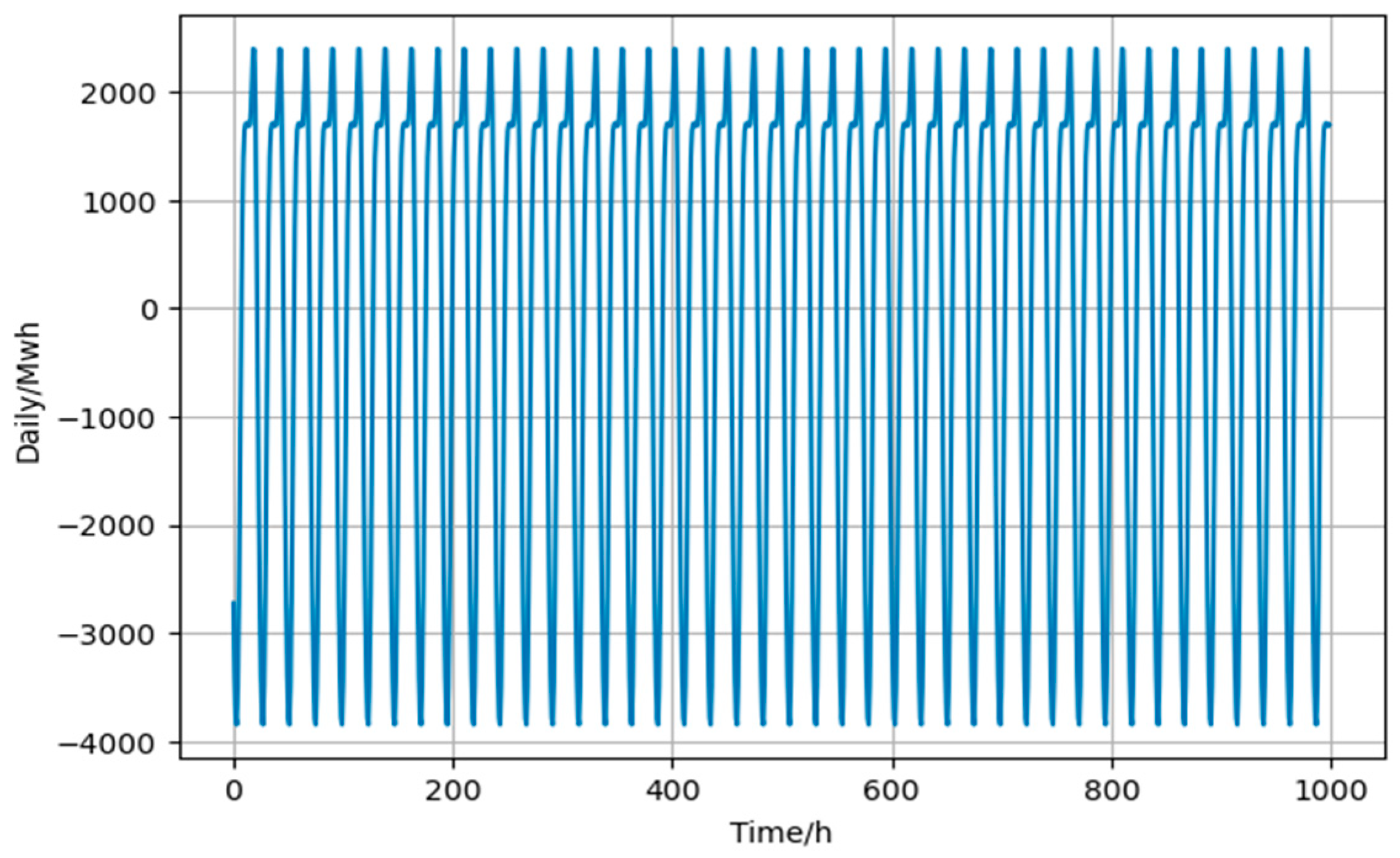
This paper adopts the Prophet algorithm to extract trend features, which illustrates the periodic variation trend in the trend features of electricity load data, as depicted in Figure 3. Simultaneously, the daily and weekly cycle features, along with residuals, are extracted from the electricity load data, as shown in Figure 4 and Figure 5. Specifically, Figure 4 presents the localized view of the daily cycle feature, providing the clearer depiction of the 24 h periodic variation. Figure 5 presents the localized view of the weekly cycle feature, highlighting the 24 × 7 h periodic variation. The residuals are obtained after extracting the trend and cycle information. The result of the CEEMDAN decomposition is shown in Figure 6, presenting the decomposition of the residuals into 14 Intrinsic Mode Functions (IMFs).

3.1.3. Input Matrix

The electricity load data are not only influenced by the current state but also by the preceding moments. Consequently, this paper utilizes a sliding window to construct a data matrix as input for the forecasting model. The calculation process is outlined as follows:
X = x 1 1 x 1 2 x 1 n x 2 1 x 2 2 x 2 n x m 1 x m 2 x m n
Y = y 1 y 2 y m
( y t + 1 , y t + 2 , , y 2 t ) = f x 1 1 x 1 2 x 1 n x 2 1 x 2 2 x 2 n x m 1 x m 2 x m n  
( y t + 2 , y t + 3 , , y 2 t + 1 ) = f x 2 1 x 2 2 x 2 n x 3 1 x 3 2 x 3 n x t + 1 1 x t + 1 2 x t + 1 n  
where x t n denotes the feature values, which are derived from the decomposition of electricity load data. n denotes the number of features for each data point, and m denotes the total number of data points. y t stands for the actual electricity load data, t represents the sliding window length, f denotes the forecasting method, and ( y t + 1 , y t + 2 , , y 2 t ) represents the forecasting value. The forecasting process is illustrated in Figure 7.

3.1.4. Model Settings

This paper uses the mean absolute error (MAE), mean absolute percentage error (MAPE) and root mean square error (RMSE) for performance comparison.
M A E = 1 N i = 1 N y i y i ^ ,
M A P E = 1 N i = 1 N y i y i ^ y i ,
R M S E = 1 N i = 1 N y i y i ^ ,
where y i ^ is the forecasted load value, y i is the actual load value, and N is the number of samples.

3.1.5. Model Settings

The paper compares three models including LSTM, Prophet-LSTM, and Prophet-EEMD-LSTM, validating the performance of the Prophet-CEEMDAN-ARBiLSTM. The parameters of these models are summarized as follows:
(1)
Prophet-GRU [32]: The model first employs the Prophet approach to decompose the input series, yielding the trend components, periodic components, and residual terms. Then, GRU is used to learn the temporal information of the above components to obtain the final output. The unit size of GRU is 32. The dropout rate is set as 0.1, and the learning rate is 0.001 in this paper.
(2)
Prophet-LSTM [33]: Different from the Prophet-GRU, LSTM is used to capture the long- and short-term dependencies from input data. The unit size of LSTM is 32 in this paper. For dropout, the dropout rate is set as 0.1. The learning rate is 0.001.
(3)
Prophet-EEMD-LSTM [33]: Different from above method, the Prophet-EEMD-LSTM adopts the EEMD to decompose the residual data, producing the multiple Intrinsic Mode Functions (IMFs) and the final residue. Then, the above components are used as the input of the LSTM to produce the final output. The unit size of LSTM is 16. For dropout, the dropout rate is set as 0.1. The learning rate is 0.001.
(4)
Prophet-CEEMDAN-ARBiLSTM: Different from the Prophet-EEMD-LSTM, the CEEMDAN method promotes the performance of the model to recognize the complex signals, thereby improving the sensitivity to the intricate information. In addition, the designed ARBiLSTM can help the model learn the temporal features influencing the variation in the load sequence and produce more accurate forecasting results. The unit size of BiLSTM in the ARBiLSTM block is 16. For dropout, the dropout rate is set as 0.1. The learning rate is 0.001.

3.2. Effectiveness Evaluation of Proposed Method

The forecasting accuracy of the whole proposed method is compared with the proposed method removing CEEMDAN (Prophet-ARBiLSTM), the proposed method removing Prophet (CEEMDAN-ARBiLSTM), and the proposed method removing ARBiLSTM (Prophet-CEEMDAN-Dense), validating the effectiveness of the Prophet-CEEMDAN-ARBiLSTM model. Figure 8 illustrates the training losses of these methods. Compared to Prophet-ARBiLSTM, CEEMDAN-ARBiLSTM, and Prophet-CEEMDAN-Dense, the Prophet-CEEMDAN-ARBiLSTM model demonstrates a significant reduction in training loss. It indicates that the forecasted model incorporating Prophet, CEEMDAN, and ARBiLSTM indeed enhances forecasting performance significantly.
This study further compares the next 24 h forecasting value of different modules in Prophet-CEEMDAN-ARBiLSTM on the test set, as presented in Table 1. Comparing the data from rows 1 and 4, it is evident that the ARBiLSTM block significantly contributes to the forecasting performance. The MAPE, MAE, and RMSE exhibit reductions of 3.83%, 578.11, and 760.82, respectively. The enhanced performance can be attributed to the residual connections and BiLSTM. Through these connections, temporal information is directly propagated to the subsequent BiLSTM layer, enabling the extraction of temporal features from adjacent and preceding layers, thereby promoting performance. Moreover, comparing the data from rows 3 and 4, it is apparent that the Prophet algorithm demonstrates notable performance in reducing forecasting errors, with MAPE, MAE, and RMSE decreasing by 0.71%, 112.35, and 143.57, respectively. It indicates that the Prophet algorithm can learn the periodic and trend information, thereby enhancing the model generalization ability. Finally, the comparison of rows 2 and 4 demonstrates that the utilization of the CEEMDAN algorithm can result in the reduction in the forecasting errors, with MAPE, MAE, and RMSE decreasing by 1.34%, 216.28, and 324.93, respectively.

3.3. Comparison with Other Existing Models

The paper compares the forecasting values with the existing methods, validating the forecasting accuracy of the models. Simultaneously, the sliding window t is set to 24 for predicting the load of the next 24 h, and the resulting curve of the models is depicted in Figure 9. It can be observed from Figure 9 that the MAE values of ARIMA and ETS are higher than other benchmark models at most time points. This shows that the above models can only capture the overall trend of load change in one day, and they cannot identify the fine change in load series.
The MAE values of Prophet-LSTM and Prophet-GRU are close at most time points. It demonstrates that the Prophet-LSTM can effectively leverage the historical electricity load data to forecast future load values, yielding an accurate forecasted result. However, the LSTM method cannot accurately fit the volatile load data, leading to the reduction in the forecasting accuracy. The Prophet-GRU can enhance the performance of the electricity load. Nevertheless, it struggles to precisely capture the random features of the load data, limiting the forecasting performance. The Prophet-EEMD-LSTM model employs EEMD to mitigate uncertainty in electricity load data, but there is room for improvement in extracting random load features. It can be observed from Figure 9 that the MAE values of Prophet-CEEMDAN-ARBiLSTM are lower than those of Prophet-EEMD-LSTM at most time points. It shows that the Prophet-CEEMDAN-ARBiLSTM adopts the CEEMDAN method to decompose the uncertain input data, effectively forecasting the uncertain changing trends. Moreover, the ARBiLSTM block extracts temporal features influencing load variations from the input series. Consequently, Prophet-CEEMDAN-ARBiLSTM produces accurate forecasting results.
The proposed method is compared with Prophet-LSTM, Prophet-GRU, and Prophet-EEMD-LSTM to validate the performance of Prophet-CEEMDAN-ARBiLSTM, as presented in Table 2. It can be seen that the most superior accuracy is found with the Prophet-CEEMDAN-ARBiLSTM model. Compared to Prophet-EEMD-LSTM, the performance metrics show a reduction of 0.26% in MAPE, a decrease of 48.94 in MAE, and a decrease of 79.76 in RMSE. Compared to Prophet-LSTM, the reductions are 1.61% in MAPE, 258.45 in MAE, and 375.58 in RMSE. Compared to Prophet-GRU, the reductions are 1.57% in MAPE, 254.23 in MAE, and 370.6 in RMSE. These results indicate that Prophet-CEEMDAN-ARBiLSTM effectively leverages the strengths of Prophet, CEEMDAN, and ARBiLSTM, thereby promoting generalization ability.
Figure 10 illustrates the MAE comparison for the models across different seasons. It can be observed from Figure 10a that each model possesses a large MAE from 5 a.m. to 7 a.m. However, the MAE values of the proposed method and Prophet-EEMD-LSTM are significantly lower than those of other benchmark models. Figure 10b shows that the benchmark models have a large MAE from 12 a.m. to 3 p.m., indicating that they struggle to accurately forecast the minimum electricity load. In contrast, Prophet-CEEMDAN-ARBiLSTM demonstrates lower MAE values during this period. The reason is that the Prophet and CEEMDAM method effectively decomposes the components that capture the load variation. Additionally, the ARBiLSTM can learn temporal features affecting changes in load data. Figure 10c shows that Prophet-LSTM and Prophet-GRU exhibit significant MAE from 11 a.m. to 5 p.m. The reason is that the features extracted by Prophet cannot accurately learn the change trend of the electricity load. Compared with these models, the proposed model and Prophet-EEMD-LSTM can produce more accurate forecast results. Figure 10d demonstrates that Prophet-GRU produces a large forecasting error at 3 p.m., indicating the challenge in forecasting the maximum load. In summary, Prophet-CEEMDAN-ARBiLSTM achieves a low MAE. It indicates that Prophet-CEEMDAN-ARBiLSTM can effectively forecast the electricity load data of different seasons. Figure 11 shows that the proposed method effectively fits actual electricity load data on the weekdays and weekends. These experiments show that Prophet-CEEMDAN-ARBiLSTM outperforms other models during various time periods, highlighting its high generalization capability.

4. Conclusions

The paper proposes a novel load forecasting model, Prophet-CEEMDAN-ARBiLSTM, for predicting the load of the next day. The ARBiLSTM block enhances forecasting accuracy and mitigates the gradient vanishing issue. Additionally, this paper tests the generalization ability of different models on the New England dataset.
The results indicate that Prophet-CEEMDAN-ARBiLSTM combines the strengths of Prophet, CEEMDAN, and BiLSTM. Moreover, it outperforms existing models in forecasting performance across different time periods. However, this paper only considers a single forecasting factor, limiting the model’s generalization ability. Future research should incorporate additional information such as temperature, humidity, and calendar information to enhance forecasting ability.

Author Contributions

Conceptualization, J.Y.; Data curation, X.Z.; Funding acquisition, J.Y.; Investigation, J.Y.; Resources, F.R.; Software, X.Z.; Writing—original draft preparation, W.C. All authors have read and agreed to the published version of the manuscript.

Funding

This research was funded by Electric Power Science Research Institute, Yunnan Power Grid Co., Ltd., grant number 0562002023030301PD00004.

Data Availability Statement

Public datasets were applied in the paper. These data can be found here: https://www.iso-ne.com/isoexpress/web/reports/load-and-demand/ (accessed on 5 November 2023).

Conflicts of Interest

Jindong Yang and Xiran Zhang are hired by the Yunnan Power Grid Co., Ltd. The authors declare that no conflicts of interest exist in the paper.

References

  1. Guo, Y.; Li, Y.; Qiao, X.; Zhang, Z.; Zhou, W.; Mei, Y.; Lin, J.; Zhou, Y.; Nakanishi, Y. BiLSTM Multitask Learning-Based Combined Load Forecasting Considering the Loads Coupling Relationship for Multienergy System. IEEE Trans. Smart Grid. 2022, 13, 3481–3492. [Google Scholar] [CrossRef]
  2. Sharma, A.; Sachin, K.J. A Novel Two-Stage Framework for Mid-Term Electric Load Forecasting. IEEE Trans. Ind. Informat. 2024, 20, 247–255. [Google Scholar] [CrossRef]
  3. Dong, J.; Luo, L.; Lu, Y.; Zhang, Q. A Parallel Short-Term Power Load Forecasting Method Considering High-Level Elastic Loads. IEEE Trans. Instrum. Meas. 2023, 72, 1–10. [Google Scholar] [CrossRef]
  4. Wang, C.; Zhou, Y.; Wen, Q.; Wan, Y. Improving Load Forecasting Performance via Sample Reweighting. IEEE Trans. Smart Grid. 2023, 14, 3317–3320. [Google Scholar] [CrossRef]
  5. Zhao, P.; Cao, D.; Wang, Y.; Chen, Z.; Hu, W. Gaussian Process-Aided Transfer Learning for Probabilistic Load Forecasting Against Anomalous Events. IEEE Trans. Power Syst. 2023, 38, 2962–2965. [Google Scholar] [CrossRef]
  6. Xiao, J.W.; Liu, P.; Fang, H.; Liu, X.K.; Wang, Y.W. Short-Term Residential Load Forecasting with Baseline-Refinement Profiles and Bi-Attention Mechanism. IEEE Trans. Smart Grid. 2024, 15, 1052–1062. [Google Scholar] [CrossRef]
  7. Conejo, A.; Plazas, M.; Espinola, R.; Molina, A. Day-ahead electricity price forecasting using the wavelet transform and ARIMA models. IEEE Trans. Power Syst. 2005, 20, 1035–1042. [Google Scholar] [CrossRef]
  8. Mariana, R.M.; Laurențiu, D.M.; Ștefanesc, V. Studies on energy consumption using methods of exponential smoothing. In Proceedings of the International Symposium on Advanced Topics in Electrical Engineering (ATEE), Bucharest, Romania, 28–30 March 2019; pp. 1–4. [Google Scholar]
  9. Elsaraiti, M.; Ali, G.; Musbah, H.; Merabet, A.; Little, T. Time series analysis of electricity consumption forecasting using ARIMA model. In Proceedings of the 2021 IEEE Green Technologies Conference (GreenTech), Denver, CO, USA, 7–9 April 2021; pp. 259–262. [Google Scholar]
  10. Dittmer, C.; Lemmer, A. Power demand forecasting for demand-driven energy production with biogas plants. Renew. Energy 2021, 163, 1871–1877. [Google Scholar] [CrossRef]
  11. Goudarzi, S.; Anisi, M.H.; Kama, N. Predictive modelling of building energy consumption based on a hybrid nature-inspired optimization algorithm. Energy Build. 2019, 196, 83–93. [Google Scholar] [CrossRef]
  12. Jagait, R.K.; Fekri, M.N.; Grolinger, K.; Mir, S. Load Forecasting Under Concept Drift: Online Ensemble Learning with Recurrent Neural Network and ARIMA. IEEE Access. 2021, 9, 98992–99008. [Google Scholar] [CrossRef]
  13. Wang, R.; Zhang, W.; Deng, W.; Zhang, R.; Zhang, X. Study on prediction of energy conservation and carbon reduction in universities based on exponential smoothing. Sustainability 2022, 14, 11903. [Google Scholar] [CrossRef]
  14. Wu, Z.; Zhao, X.; Ma, Y.; Zhao, X. A hybrid model based on modified multi-objective cuckoo search algorithm for short-term load forecasting. Appl. Energy 2019, 237, 896–909. [Google Scholar] [CrossRef]
  15. Wu, D.; Wang, B.; Precup, D.; Boulet, B. Multiple kernel learning based transfer regression for electric load forecasting. IEEE Trans. Smart Grid. 2020, 11, 1183–1192. [Google Scholar] [CrossRef]
  16. Cordeiro, C.M.; Villanueva, D.; Eguía, O.P.; Martínez, C.M.; Ramos, S. Load Forecasting with Machine Learning and Deep Learning Methods. Appl. Sci. 2023, 13, 7933. [Google Scholar] [CrossRef]
  17. Zhang, Z.; Dong, Y.; Hong, W.C. Long Short-Term Memory-Based Twin Support Vector Regression for Probabilistic Load Forecasting. IEEE Trans. Neural Netw. Learn. Syst. 2023, 1–15. [Google Scholar] [CrossRef] [PubMed]
  18. Li, Y.; Zhu, N.; Hou, Y. A novel hybrid model for building heat load forecasting based on multivariate Empirical modal decomposition. Build. Environ. 2023, 237, 110317. [Google Scholar] [CrossRef]
  19. Sayed, H.A.; William, A.; Said, A.M. Smart Electricity Meter Load Prediction in Dubai Using MLR, ANN, RF, and ARIMA. Electronics 2023, 12, 389. [Google Scholar] [CrossRef]
  20. Jiang, H.; Zhang, Y.; Muljadi, E.; Zhang, J.J.; Gao, D.W. A Short-Term and High-Resolution Distribution System Load Forecasting Approach Using Support Vector Regression with Hybrid Parameters Optimization. IEEE Trans. Smart Grid. 2018, 9, 3341–3350. [Google Scholar] [CrossRef]
  21. Chen, Y.; Xu, P.; Chu, Y.; Li, W.; Wu, Y.; Ni, L.; Bao, Y.; Wang, K. Short-Term Electrical Load Forecasting Using the Support Vector Regression (SVR) Model to Calculate the Demand Response Baseline for Office Buildings. Appl. Energy 2017, 195, 659–670. [Google Scholar] [CrossRef]
  22. Jian, L.; Daiyu, D.; Junbo, Z.; Dong, C.; Wei, H. A Novel Hybrid Short-Term Load Forecasting Method of Smart Grid Using MLR and LSTM Neural Network. IEEE Trans. Ind. Inform. 2021, 17, 2443–2452. [Google Scholar]
  23. Lu, H.; Cheng, F.; Ma, X. Short-term prediction of building energy consumption employing an improved extreme gradient boosting model: A case study of an intake tower. Energy 2020, 203, 117756. [Google Scholar] [CrossRef]
  24. Liu, Z.; Yu, J.; Feng, C.; Su, Y.; Dai, J.; Chen, Y. A hybrid forecasting method for cooling load in large public buildings based on improved long short-term memory. J. Build. Eng. 2023, 76, 107238. [Google Scholar] [CrossRef]
  25. Rubasinghe, O.; Zhang, X.; Chau, T.K.; Chow, Y.H.; Fernando, T. A Novel Sequence to Sequence Data Modelling Based CNN-LSTM Algorithm for Three Years Ahead Monthly Peak Load Forecasting. IEEE Trans. Power Syst. 2020, 39, 1932–1947. [Google Scholar] [CrossRef]
  26. Chaojie, L.; Zhao, D.; Lan, D.; Henry, P.; Zihang, Q.; Guo, C.; Deo, P. Interpretable Memristive LSTM Network Design for Probabilistic Residential Load Forecasting. IEEE Trans. Circuits Syst. I Regul. Pap. 2022, 69, 2297–2310. [Google Scholar]
  27. Muzumdar, A.A.; Modi, C.N.; Vyjayanthi, C. Designing a Robust and Accurate Model for Consumer-Centric Short-Term Load Forecasting in Microgrid Environment. IEEE Syst. J. 2022, 16, 2448–2459. [Google Scholar] [CrossRef]
  28. Liu, Y.; Liang, Z.; Li, X. Enhancing Short-Term Power Load Forecasting for Industrial and Commercial Buildings: A Hybrid Approach Using TimeGAN, CNN, and LSTM. IEEE Open J. Ind. Electron. Soc. 2023, 4, 451–462. [Google Scholar] [CrossRef]
  29. Ijaz, K.; Hussain, Z.; Ahmad, J.; Ali, S.F.; Adnan, M.; Khosa, I. A Novel Temporal Feature Selection Based LSTM Model for Electrical Short-Term Load Forecasting. IEEE Access. 2022, 10, 82596–82613. [Google Scholar] [CrossRef]
  30. Shakeel, A.; Chong, D.; Wang, J. District heating load forecasting with a hybrid model based on LightGBM and FB-prophet. J. Clean. Prod. 2023, 409, 137130. [Google Scholar] [CrossRef]
  31. Kim, T.Y.; Cho, S.B. Research on Peak Load Prediction of Distribution Network Lines Based on Prophet-LSTM Model. Sustainability 2023, 15, 11667. [Google Scholar] [CrossRef]
  32. Son, N.; Shin, Y. Short-and Medium-Term Electricity Consumption Forecasting Using Prophet and GRU. Sustainability 2023, 15, 15860. [Google Scholar] [CrossRef]
  33. Lu, Y.; Sheng, B.; Fu, G.; Luo, R.; Chen, G.; Huang, Y. Prophet-EEMD-LSTM based method for predicting energy consumption in the paint workshop. Appl. Soft Comput. 2023, 143, 110447. [Google Scholar] [CrossRef]
  34. Ko, M.S.; Lee, K.; Kim, J.K.; Hong, C.W.; Dong, Z.Y.; Hur, K. Deep Concatenated Residual Network with Bidirectional LSTM for One-Hour-Ahead Wind Power Forecasting. IEEE Trans. Sustain. Energy 2021, 12, 1321–1335. [Google Scholar] [CrossRef]
  35. Li, K.; Huang, W.; Hu, G. Ultra-short term power load forecasting based on CEEMDAN-SE and LSTM neural network. Energy Build. 2023, 279, 112666. [Google Scholar] [CrossRef]
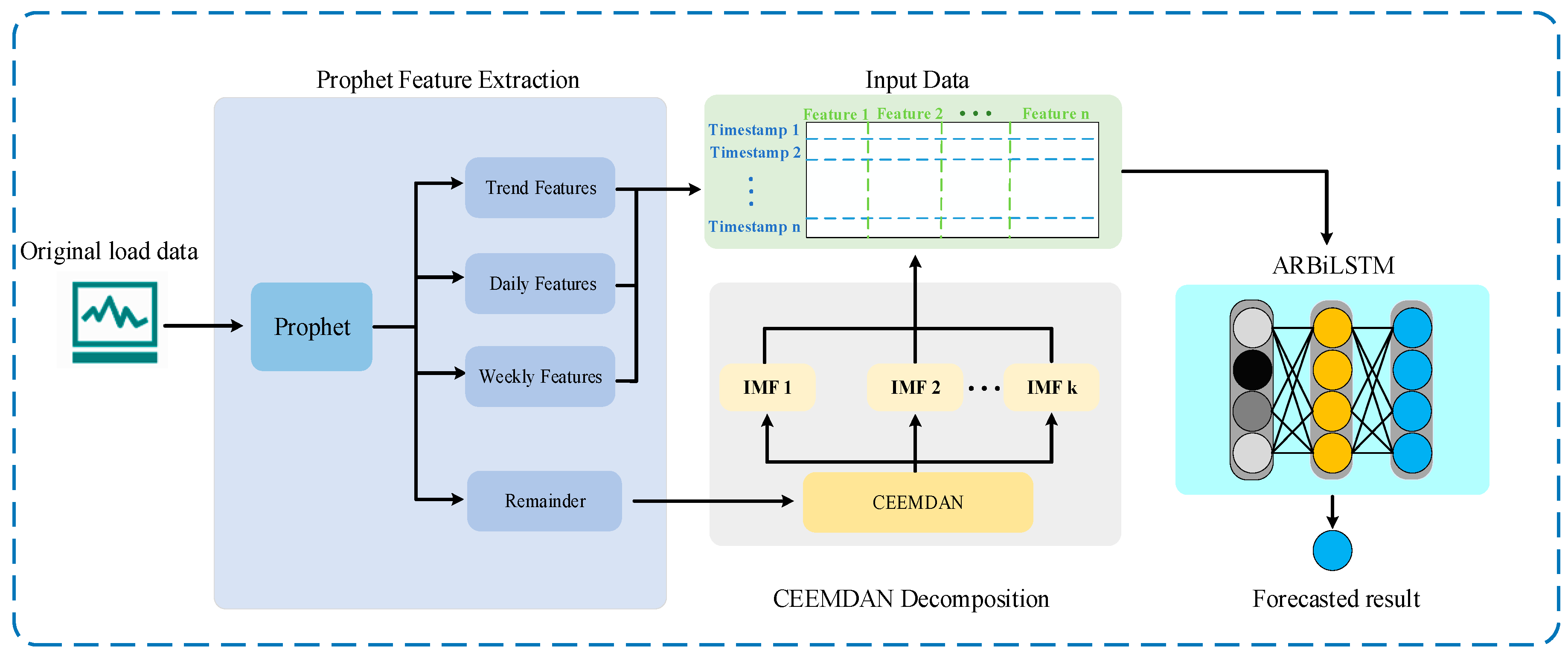
Figure 1. The proposed forecast method, including Prophet, CEEMDAN, and ARBiLSTM block.
Futureinternet 16 00192 g001
Figure 2. Advanced residual BiLSTM (ARBiLSTM): BN, batch normalization; BiLSTM, Bidirectional Long Short-Term Memory layer.
Futureinternet 16 00192 g002
Figure 3. Trend feature data.
Futureinternet 16 00192 g003
Figure 4. Part of daily feature data.
Futureinternet 16 00192 g004
Figure 5. Part of weekly feature data.
Futureinternet 16 00192 g005
Figure 6. CEEMDAN decomposition results.
Futureinternet 16 00192 g006
Figure 7. Sliding window to produce the input–output matrix.
Futureinternet 16 00192 g007
Figure 8. The losses of the Prophet-ARBiLSTM, the CEEMDAN-ARBiLSTM, the Prophet-CEEMDAN-Dense, and the Prophet-CEEMDAN-ARBiLSTM.
Futureinternet 16 00192 g008
Figure 9. Forecast error comparison of the methods in one year.
Futureinternet 16 00192 g009
Figure 10. Forecast error comparison of the methods in different seasons. (a) Spring. (b) Summer. (c) Autumn. (d) Winter.
Futureinternet 16 00192 g010
Figure 11. Forecast results comparison of the methods on weekday and weekend. (a) Weekday. (b) Weekend.
Futureinternet 16 00192 g011
Table 1. Effectiveness validation of the modules on the test set.
MethodMAPE (%)MAE (Mwh)RMSE (Mwh)
Prophet-CEEMDAN-Dense5.49812.681091.77
Prophet-ARBiLSTM3.00450.85655.88
CEEMDAN-ARBiLSTM2.37346.92474.52
Prophet-CEEMDAN-ARBiLSTM1.66234.57330.95
Table 2. Performance comparison of the different methods.
MethodMAPE (%)MAE (Mwh)RMSE (Mwh)
ARIMA7.731138.591364.69
ETS5.47814.561095.98
Prophet-LSTM3.27493.02706.53
Prophet-GRU3.23488.8701.55
Prophet-EEMD-LSTM1.92283.51410.71
Prophet-CEEMDAN-ARBiLSTM1.66234.57330.95
Disclaimer/Publisher’s Note: The statements, opinions and data contained in all publications are solely those of the individual author(s) and contributor(s) and not of MDPI and/or the editor(s). MDPI and/or the editor(s) disclaim responsibility for any injury to people or property resulting from any ideas, methods, instructions or products referred to in the content.