Refined Semi-Supervised Modulation Classification: Integrating Consistency Regularization and Pseudo-Labeling Techniques

Abstract

Automatic modulation classification (AMC) plays a crucial role in wireless communication by identifying the modulation scheme of received signals, bridging signal reception and demodulation. Its main challenge lies in performing accurate signal processing without prior information. While deep learning has been applied to AMC, its effectiveness largely depends on the availability of labeled samples. To address the scarcity of labeled data, we introduce a novel semi-supervised AMC approach combining consistency regularization and pseudo-labeling. This method capitalizes on the inherent data distribution of unlabeled data to supplement the limited labeled data. Our approach involves a dual-component objective function for model training: one part focuses on the loss from labeled data, while the other addresses the regularized loss for unlabeled data, enhanced through two distinct levels of data augmentation. These combined losses concurrently refine the model parameters. Our method demonstrates superior performance over established benchmark algorithms, such as decision trees (DTs), support vector machines (SVMs), pi-models, and virtual adversarial training (VAT). It exhibits a marked improvement in the recognition accuracy, particularly when the proportion of labeled samples is as low as 1–4%.

1. Introduction

In the modern era of digital interconnectedness, wireless communication systems are pivotal in forging effective channels that link individuals, devices, and data across vast distances [1,2]. These systems, dependent on the transmission and reception of signals, are critical for seamless communication. Initially, the field of wireless communication was characterized by a restricted suite of modulation schemes and a cooperative nature, where entities engaged in communication mutually agreed on the schemes to be employed. This era did not demand signal recognition at the receiving end. As wireless communication systems have progressed, expanding in diversity and intricacy, the implementation of multiple modulation schemes has become commonplace. This development underscores the need for precise classification of these varied schemes, a task skillfully managed by automatic modulation classification (AMC) [3,4]. AMC has an integral role in non-cooperative communication scenarios, acting as a link between signal detection and demodulation. Here, non-cooperative communication refers to instances where an external party gains access to a communication system with no prior approval from the original communicating parties, without affecting their ongoing communication. AMC’s utility spans military and civilian sectors. In military applications, it is instrumental in identifying and analyzing electromagnetic signals, which can reveal the functionalities of enemy electronics and assess their threat levels. Moreover, AMC processes this intelligence, bolstering reconnaissance efforts. In civilian applications, AMC’s ability to distinguish between modulation schemes is fundamental to efficient device communication and vital for smart, efficient, and reliable systems. A clear example is in smart home ecosystems, where wireless communication integrates smart appliances and security systems. Through AMC, these devices can discern and accurately process communication signals, ensuring secure data transmission and operational reliability.

In situations where many parameters of the transmitted data and receiver are not known, such as signal power, carrier frequency, and phase offset, automatic modulation classification is a challenging task [5]. Traditional methods can be broadly grouped into two categories: likelihood theory-based AMC (LB-AMC) [6,7,8] and feature-based AMC (FB-AMC) [9,10,11]. The pivotal concept underlying the LB-AMC method involves establishing a likelihood function based on the statistical attributes of the signal model. This determines an optimal discrimination threshold. By evaluating the signal’s likelihood ratio against the threshold, a modulation scheme can be identified. LB-AMC has been shown to achieve optimal performance in Bayesian estimation, as it minimizes the probability of erroneous classification. Nevertheless, its elevated computational complexity poses a challenge to its practical adoption, as it may not satisfy the requirements of real-time processing and a low cost. Notably, when the parameters remain unknown, the recognition accuracy may be significantly affected. Currently, the FB-AMC method has emerged as the predominant approach. Its main principle is to select suitable features and carry out feature extraction from the received signal. Subsequently, a trained classifier classifies the extracted feature information. In comparison with LB-AMC, its algorithm complexity is significantly diminished. In particular, it can be perceived as a mapping relationship from the signal space to the feature space. It morphs a high-dimensional signal space into a lower-dimensional feature space, simplifying calculations. Additionally, the features extracted from the received signal can exhibit differences between diverse modulation schemes. The features should be precise to achieve superior recognition performance. Selection of excellent statistical features is paramount for FB-AMC. The features selected can be grouped into the following categories: time-domain features based on instantaneous amplitude, phase, and frequency [12]; frequency-domain features based on a cyclic spectrum [13] and higher-order cumulants [14]; and transform-domain features based on constellation diagrams [15] and wavelet transforms [16]. Traditional classifiers like support vector machines (SVMs) [17] and decision tree (DT) [18] struggle to learn complex feature representations from data. In addition, feature extraction necessitates artificial design, which lead to significant human resource engagement. Feature engineering is indeed a laborious task requiring specialized expertise. Most crucially, the designed features may be confined to specific modulation schemes.

Deep learning algorithms have demonstrated substantial advantages in applications such as image recognition, speech recognition, and facial recognition. Concurrently, they are employed in the field of wireless communication for tasks like spectrum prediction [19], specific emitter identification [20,21,22,23,24], and automatic modulation classification [25,26]. Deep learning AMC (DL-AMC) methods are data-driven approaches [26]. The depth of the network used is much deeper than the previous network. This allows them to extract more complex features. Unlike previous approaches, it can automatically extract features from raw data and makes effective decisions without manual intervention. These methods include convolutional neural networks (CNNs) [27,28] and recurrent neural networks (RNNs) [29]. The core idea of a CNN is to extract features from input data through a series of convolution layers, pooling layers, and fully connected layers. An RNN is a deep learning model that excels in processing sequential data. Its core idea is to introduce recurrent units into the network, making the output of the network dependent not only on the current step but also on the output of the previous step. For deep learning methods, sample annotation is expensive and their performance highly depends on the quality of the data.

Motivated by this, some methods such as few-shot learning [30], conditional generative adversarial networks (CGANs) [31], and semi-supervised learning have been considered. Few-shot learning’s objective is to develop precise models with fewer samples. A CGAN is a type of generative adversarial network that involves the conditional generation of images by a generator model. This enables discernible image generation of a specified type. Semi-supervised learning employs minimal labeled data, coupled with substantial unlabeled data for training, as shown in Figure 1. In this paper, we propose a semi-supervised automatic modulation classification (SSL-AMC) method based on consistency regularization and pseudo-labeling. Consistency regularization effectively mitigates overfitting by requiring model output consistency amidst slight data variations. The common method is input perturbation, which involves making small random changes to input data. This can encourage the model to produce stable responses to minor variations. Pseudo-labeling is a semi-supervised learning method that leverages the model’s predictions on unlabeled data and adds them as pseudo-labels to the unlabeled data, overcoming the problem of sparsely labeled data. We use a wide residual network (WRN) as a backbone network. A WRN is a variant of convolution neural networks that introduces a wider network structure based on residual networks; i.e., it increases the number of channels. Our experimental results demonstrate that the proposed method achieves a high recognition accuracy with limited labeled signal samples. The main contributions of this paper are summarized as follows:

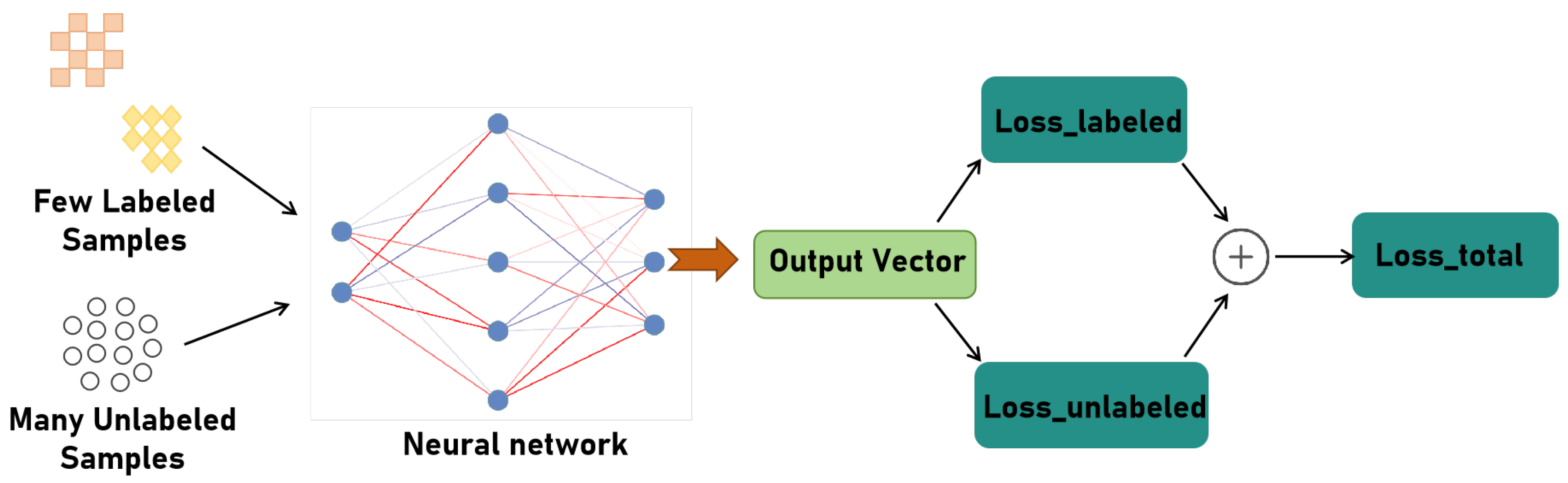
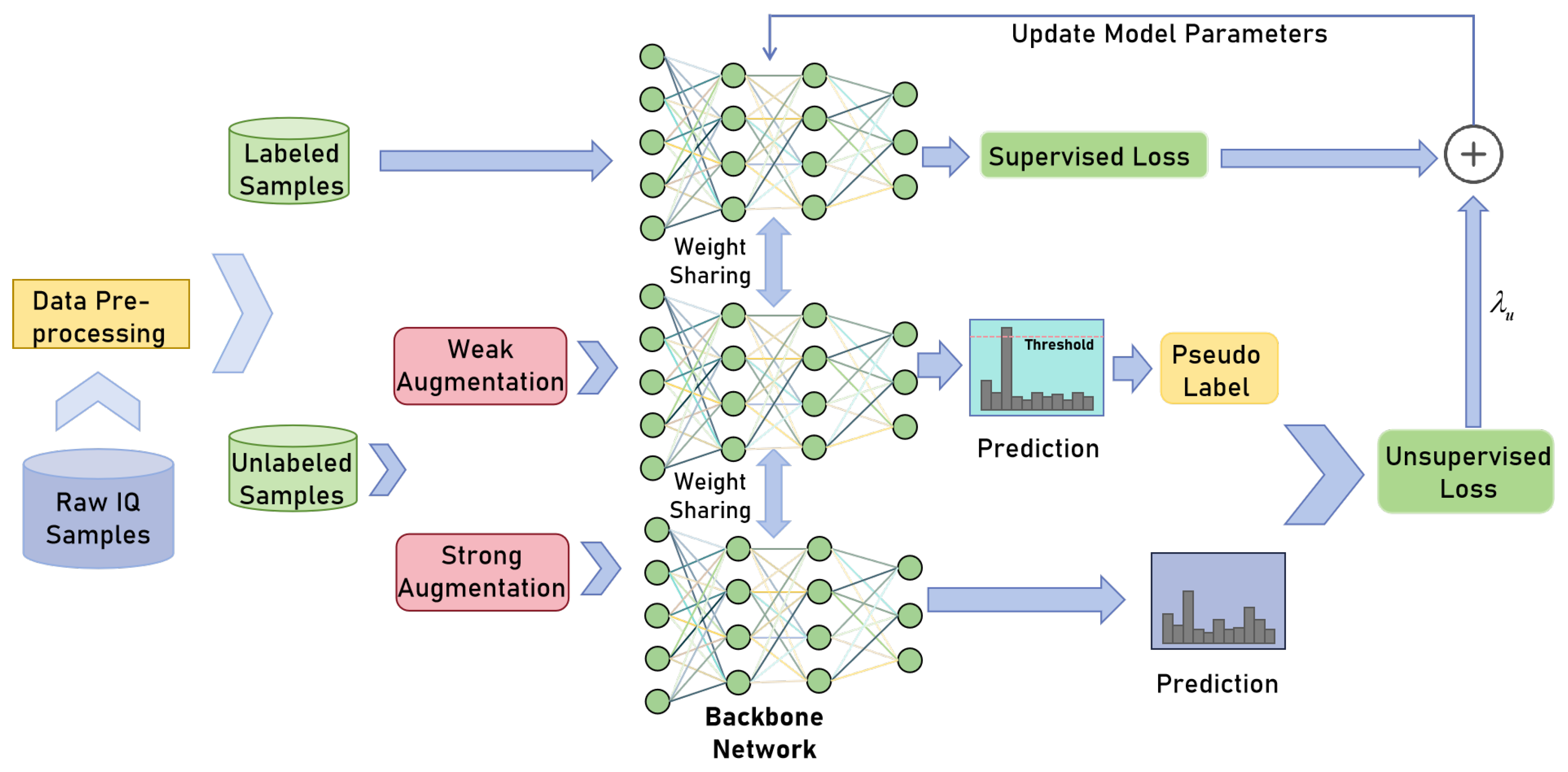
• We present a semi-supervised AMC method based on consistency regularization and pseudo-labeling. Consistency regularization is used to encourage the model to extract generalized features from the signal data. Pseudo-labeling is used to make manual predictions for unlabeled data. Both methods are alternatively used to improve the identification performance.

2. Related Works

2.1. Traditional AMC Methods

The likelihood-theory-based approach is proposed, which introduces the basic concept of the likelihood function and explains how to build likelihood functions from the known statistical properties of a signal. It also discusses how to apply the likelihood ratio method under different channel conditions. As a result of the computational complexity of LB-AMC, researchers have turned their attention to FB-AMC. Many feature extraction algorithms, such as cyclic features, high-order moments, and high-order cumulants, and transform domain features, such as wavelet transforms, exist. Azzouz et al. [32] select time-domain features such as instantaneous frequency, amplitude, and phase to extract the features. Their method achieves the identification of modulation schemes such as ASK, BPSK, and FSK. Y. Han et al. [33] select second-order, fourth-order, sixth-order, and eighth-order cyclic cumulants as features. This method achieves recognition of modulation schemes such as ASK, BPSK, QAM, and APSK. C. Chou et al. [34] choose constellation images as the feature; different modulation schemes present different distribution shapes and densities in constellation images. This method can identify BPSK, QPSK, and 8PSK in the presence of inter-symbol interference (ISI). S. Li et al. [35] choose the cyclic spectrum and the quadratic cyclic spectrum as features. The cyclic spectrum can be used to detect the periodic frequency components of the signal and the quadratic cyclic spectrum is more sensitive to the nonlinear characteristics of the signal. This method can classify PSK, FSK, QAM, MSK, and OFDM modulation schemes in the presence of a multipath effect. It can be seen that the computational complexity of FB-AMC is much reduced. However, FB-AMC has a high demand for features. Feature extraction is dependent on expert experience. Researchers are searching for an algorithm that can automatically extract features.

2.2. AMC Methods Based on Deep Learning

In [36], an eye diagram of the original signal is used as an input to Lenet-5, thus linking the AMC problem to the field of image recognition. Convolutional networks for radio recognition are proposed in [37]. Simulations on the DeepSig dataset called RML2016.10A [37] show that recognition accuracy is higher than that of FB-AMC. The RML2016.10A dataset is generated based on the GNU Radio environment. The dataset includes eleven modulation signals, each of which consists of twenty signal-to-noise ratios (SNRs). Each SNR has 1000 samples. In [38], an LSTM-based AMC method is shown to outperform CNN models for small- or medium-sized received signals. In [39], long symbol rate signals are studied, and it is found that a stacked autoencoder can achieve better performance by increasing the simulation time. Wang et al. [27] design two CNNs to recognize different modulation schemes. The first CNN is trained with IQ-sampled signals. This network can distinguish QAMs from other modulation schemes; i.e., this network cannot distinguish between 16QAM and 64QAM. The second CNN is trained with a constellation image and can distinguish between 16QAM and 64QAM. Tu et al. [40] propose a novel CNN-based AMC method. They use a pruning technique to reduce the convolution parameters and the floating point operations per second (FLOPs). Experiments show that the convolution layer of this CNN, compared to the original CNN, reduces the convolution parameters without significant losses in recognition accuracy.

2.3. Semi-Supervised Learning and Its Applications

Semi-supervised learning has emerged as an imperative branch of machine learning. It seeks to enhance models using labeled and unlabeled data. Semi-supervised learning regards unlabeled data as a valuable source of information, and it is capable of amplifying the model’s generalization capability and mitigating the risk of overfitting. Semi-supervised learning is based on the notion that unlabeled data can provide additional information to model training. It enables the discovery of more comprehensive and robust feature representation. In recent years, a number of semi-supervised methods have emerged. Lee et al. [41] proposed a novel pseudo-labeling approach. The key concept of this methodology is to consider the model’s forecast of unlabeled signal samples as “labels” for unlabeled data. This approach alleviates the model overfitting problem triggered by insufficient labeled samples. Its disadvantage is that the predictive ability of the model is not strong during the initiation phase of model training. This may reduce the quality of the pseudo-labels, resulting in a decrease in recognition accuracy. Valpola et al. [42] proposed the mean teacher technique. Its core principle involves generating a teacher network by moving the average of the model parameters.

In the context of labeled data, the loss is calculated and updated through back propagation. As for unlabeled data, the loss is calculated by utilizing both the student network and teacher network. The loss is composed of two components. Supervised loss guarantees the compatibility of labeled training samples. Unsupervised loss ensures that predictions of student networks are as similar as possible to predictions of teacher networks. By carefully minimizing both parts of the loss, the generalization ability of the model can be improved. David et al. [43] integrated a variety of semi-supervised algorithms, including consistency regularization, entropy minimization, and conventional regularization techniques. Their principal goal is to implement K times data augmentation for unlabeled data. Then, K new data are acquired and K diverse predicted probability distributions are derived by feeding data into the identical classifier. These K probability distributions are averaged to obtain the average classification probability. Ultimately, the predicted labels for unlabeled data are determined using the sharp algorithm.

3. System Model and Data Preprocessing

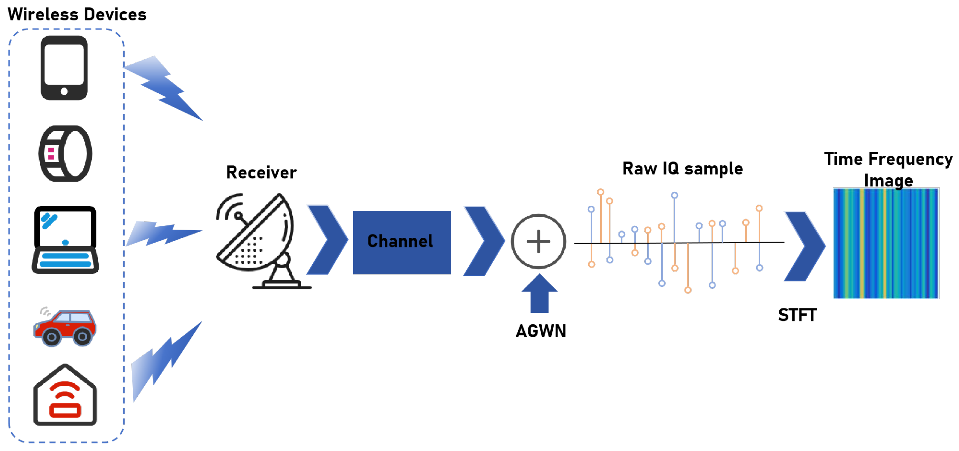
3.1. System Model

The semi-supervised-learning-based AMC system model is shown in Figure 2. At the transmitter side, the input signal $i\left(t\right)$ is modulated to obtain a modulated signal $s\left(t\right)$. The modulated signal $s\left(t\right)$ is affected by noise and channel fading during transmission. At the receiver side, the received signal $x\left(t\right)$ can be expressed as:

$$x\left(t\right)=s\left(t\right)\ast h\left(t\right)+n\left(t\right)$$

(1)

where $h\left(t\right)$ denotes the multi-path channel and ∗ stands for the convolution operation. $n\left(t\right)$ denotes additive noise. The additive noise can be broadly classified into four categories according to its source, namely radio interference, industrial noise, atmospheric interference, and internal noise. The implementation of semi-supervised AMC typically comprises three stages. Initially, we deploy receivers to receive signals from wireless devices, ideally performing data preprocessing on received signals. Here, processing involves scrutinizing and processing the acquired signals to derive an excellent representation of the signals (time-frequency images, constellation images, or more complex features). The objective is to construct more precise, robust, and comprehensive models. Subsequently, supervised and unsupervised losses are effectively constructed, independently adhering to the proposed semi-supervised algorithm. The supervised loss is derived by contrasting the predicted values of labeled samples with their authentic labels. The unsupervised loss is obtained by training on unlabeled signal samples. Specifically, two distinct levels of perturbation are implemented for unlabeled samples. Thereafter, two different probability distributions are generated by the model. The unsupervised loss is calculated by assessing these two probability distributions. Both the supervised and unsupervised losses collaboratively update the model parameters. Lastly, time-frequency signal images for the test are fed into the trained model. The model is capable of achieving the segregation of twenty modulation schemes.

3.2. Data Preprocessing

The dataset utilized in the experiment comprises twenty modulation schemes, namely BPSK, QPSK, 8PSK, 16QAM, 32QAM, 64QAM, 128QAM, 256QAM, GFSK, CPFSK, PAM4, B-FM, DSB-AM, SSB-AM, APSK, OQPSK, 2ASK, 4ASK, 2FSK, and 4FSK. Each modulation scheme contains 1000 samples. The dimension of each sample is (4096 × 2). These samples belong to the IQ sequence signal. Given the outstanding achievements of deep learning in the image recognition field, numerous research methodologies have adapted signal recognition methods for image recognition problems. Our manuscript utilizes the short-time Fourier transform (STFT) [44] to transform diverse modulated signals into the format of time-frequency images. The operating principle of the short-time Fourier transform involves separating the input signal into multiple overlapping windows. The data within each window are referred to as a frame, and the Fourier transform is applied to data within each frame to obtain information in the frequency domain. The output is a two-dimensional matrix where the horizontal axis represents time and the vertical axis represents frequency. From the time-frequency images, one can discern the energy distribution of the signal at different intervals of time and frequencies. We obtain time-frequency signal images; the dimension of each time-frequency image is (64,64,3), where 64, 64, and 3 refer to the length, width, and number of channels of the time-frequency image, respectively. The processed signal samples can be directly input into the convolution neural network. The data preprocessing process is illustrated in Figure 3.

3.3. Problem Description

Let X and Y denote the sample space and category space, respectively. $x_k\in X$ represents the input sample, i.e., signal samples with IQ format. $y\in Y$ denotes the real category corresponding to the modulation scheme.

3.3.1. AMC Problem

The automatic modulation classification task is an intermediate step between signal reception and demodulation, where the received signal is transformed into a baseband complex-valued signal sequence $X=\left\{x\right(0),x(1),\dots ,x(k-1\left)\right\}$ by the receiver. K is the number of sampling points. The received modulation signals are I/Q signals, which include a real part I and an imaginary part Q, which can be expressed as:

$$I=\left[real\right(x\left(0\right)),\dots ,real(x(K-1)\left)\right]$$

(2)

$$Q=\left[imag\right(x\left(0\right)),\dots ,imag(x(K-1)\left)\right]$$

(3)

After data preprocessing, the time-frequency image dataset $D_t={\left\{(x_i,y_i)\right\}}_{i=1}^N$. The aim of AMC is to create a mapping function $f\in F$ and to minimize its expected error.

$$\underset{f\in F}{min}{ϵ}_{ex}=\underset{f\in F}{min}{E}_{\left(x,y\right)\sim P_{X\times Y}}L\left(f\left(x\right),y\right)$$

(4)

where $L\left(f\right(x),y)$ represents the error generated by comparing the predicted value with the true label. However, the expected error cannot be calculated directly because we only have a few signal samples. In this case, we use training data to represent the entire distribution and thus calculate an approximation of the expected error.

$$\underset{f\in F}{min}{ϵ}_{em}=\underset{f\in F}{min}{E}_{\left(x,y\right)\sim D_t}L\left(f\left(x\right),y\right)$$

(5)

However, this empirical error may be affected by factors such as randomness of data sampling and noise. It cannot fully and accurately reflect the generalization ability of the model. Thus, we must take into account the difference between the expected error and the empirical error, i.e., the generalization error $ϵ=|{ϵ}_{em}-{ϵ}_{ex}|$. If the two errors are not too different, this means that the model can generalize better on both training data and unknown data. The above equation can be rewritten as:

$$\underset{f\in F}{min}{ϵ}_{em},s.t.f\left(x_i\right)=y_i,\forall (x_i,y_i)\in D_t$$

(6)

3.3.2. Semi-Supervised AMC Problem

In the semi-supervised AMC problem, the following settings were used. The training dataset is $D_t=\{(x_1,y_1),\dots ,(x_L,y_L),x_{L+1},\dots ,x_N\}$, where L is the number of labeled training samples and $N-L$ is the number of unlabeled training samples. For ease of illustration, we use $D_l=\left\{(x_l^i,y_l^i)\right|i=1,\dots ,L\}$ to denote the labeled dataset and $D_{ul}=\left\{x_{ul}^j\right|j=1,\dots ,N-L\}$ to denote the unlabeled dataset. The correlation between $D_t$, $D_l$ and $D_{ul}$ is $D_t=D_l\cup D_{ul}$, where $N-L\gg L$.

The core idea of the semi-supervised AMC problem is to find a mapping function that minimizes the expected error. In contrast to the general machine-learning-based AMC problem, due to the sparse number of labeled signal samples, we cannot compute the expected error directly. This is a frequent concern encountered in semi-supervised tasks. Information about data distribution can be obtained from unlabeled samples. Thus, in the semi-supervised AMC task, the expected error can be approximated as:

$$\underset{f\in F}{min}{ϵ}_{em}=\underset{f\in F}{min}{E}_{\left(x,y\right)\sim D_l}L(f\left(x\right),y)+\lambda E_{\left(x\right)\sim D_{ul}}{L}_{ul}\left(·\right)$$

(7)

where $L_{ul}\left(·\right)$ represents the loss obtained by training on unlabeled signal samples. The remaining portion remains identical to prior usage. Both losses utilize the cross-entropy loss function, which is a frequently utilized loss function in image classification tasks. $\lambda$ denotes the weight value of the unsupervised loss, which impacts the classification proficiency of the model to an extent. However, the aforementioned must adhere to a significant assumption that the data distribution in the unlabeled samples is useful for the AMC problem. Specifically, labeled and unlabeled data share the same label space.

4. Our Proposed Method

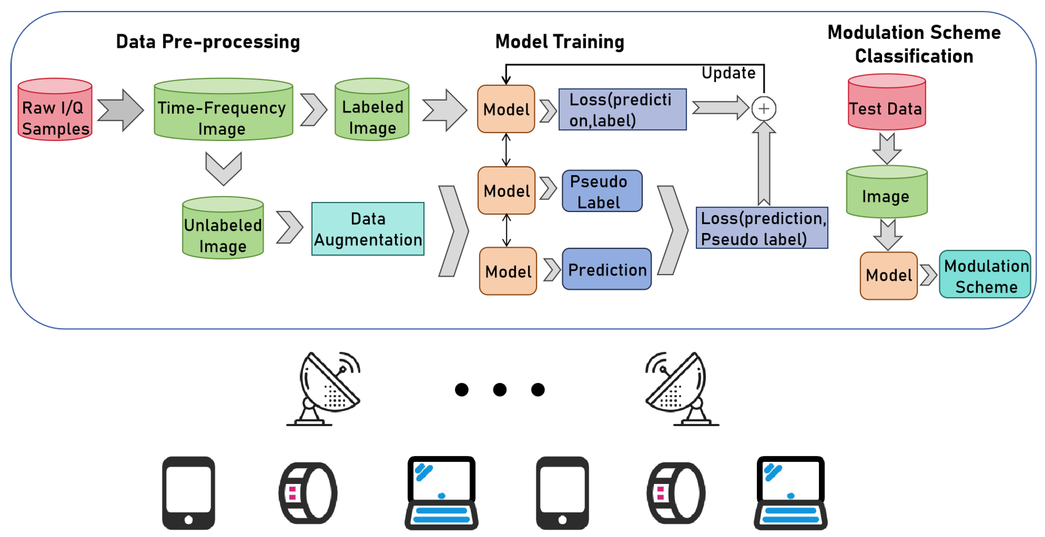
4.1. Proposed Semi-Supervised AMC Method Based on Consistency Regularization and Pseudo Labeling

The structure of our proposed semi-supervised AMC method is illustrated in Figure 4. For simplicity, our proposed method is recognized as Fixmatch. Semi-supervised learning is commonly employed for tasks where data annotation expenses are considerable or the data contain a substantial number of unlabeled samples, such as medical image analysis and agriculture and environmental surveillance. Semi-supervised learning essentially utilizes unlabeled samples to improve model performance. In this article, the fundamental concept of the proposed method is to incorporate unlabeled signal samples during model training. The specific steps are to train the model using labeled and unlabeled data, respectively, generating supervised and unsupervised losses, and backpropagating to adjust model parameters. The following discussions concentrate on how to construct supervised and unsupervised losses. The initial I/Q signals are post-processed with data to obtain the time-frequency signal images. The time-frequency signal images are divided into labeled and unlabeled signal images. The supervised loss is derived by comparing the projected value of labeled data through the model with the authentic label. It is represented as follows:

$$L_s=\frac{1}{N}\sum _{i=1}^N{L}_{ce}(y_i,P\left(y\right|x_l^i)),$$

(8)

where $P(·)$ denotes the model’s prediction, N denotes the number of labeled samples, $y_i$ denotes true labels of labeled samples, and $L_{ce}(·)$ denotes the cross-entropy loss function. It is a loss function used in classification tasks to measure the difference between model predictions and true labels.

We design unsupervised loss employing two semi-supervised methods, including consistency regularization and pseudo-labeling. We initially modify unlabeled signal samples twice with varying degrees of perturbation, which we refer to as weak data augmentation and strong data augmentation, respectively. Data augmentation is a technique that expands the training samples. The objective of data augmentation is to fortify the robustness of the model by modifying the data space. “Strong” and “weak” here denote the degree of perturbation of the data. The strong augmented and weak augmented images are fed into the model to obtain model predictions. $A(·)$ denotes strong data augmentation, which generally consists of operations including color transformation, contrast enhancement, etc. $\alpha (·)$ denotes weak data augmentation, which consists of operations including flipping. Since unlabeled samples do not possess labels, we utilize the weak augmentation branch to devise “pseudo-labels” for these unlabeled samples. The principle of pseudo-labeling [41] is to utilize the model itself to obtain artificial labels for unlabeled samples, which typically use hard labels, i.e., one-hot labels acquired by employing the argmax function. One-hot labels are only retained for labels whose maximum class probability surpasses the threshold. The formulation for pseudo-labeling is as follows:

$${\widehat{q}}_j=argmax\left(p\left(y|\alpha \left(x_{ul}^j\right)\right)\right).$$

(9)

After obtaining the pseudo-labels, we obtain model predictions for the branch of strong data augmentation. The unsupervised loss is obtained by comparing model predictions for the branch of strong data augmentation with pseudo-labels. The reason for constructing the unsupervised loss in this way is that this embodies the idea of consistency regularization. Consistency regularization is an important part of current mainstream SSL, and is based on the assumption that the same image with different perturbations through the network will output the same prediction. The unsupervised loss $L_{ul}$ can be expressed as:

$$L_{ul}=\frac{1}{N-L}\sum _{j=1}^{N-L}\mathbb{A}(max\left(p\left(y\right|\alpha \left(x_{ul}^j\right))\right)\ge \tau )L_{ce}({\widehat{q}}_j,q_j),$$

(10)

where $N-L$ represents the number of unlabeled modulation signal samples. $\tau$ denotes the confidence threshold. $\mathbb{A}(·)$ is a function. It takes the value of 1 if the maximum class probability is greater than the threshold, otherwise, it takes the value of 0. The value of the confidence threshold directly affects the quality of pseudo-labels. Setting the threshold too high results in a small number of samples used for training, and setting the threshold too low results in the introduction of a lot of erroneous information. In this paper, weak data augmentation consists of a standard flip-and-shift operation, with a 50% probability of flipping and a 12.5% probability of shifting. Employing only weak data augmentation could lead to overfitting of the training process and failure to extract crucial features. Strong data augmentation can cause severe distortion of signal images but still retains sufficient features to recognize the modulation schemes. Strong data augmentation applies the Randaugment [45] augmentation strategy and cutout [46] augmentation. The Randaugment methodology represents a variant of the Autoaugment [47] strategy, which employs a random sampling strategy to reduce the network’s dependence on the degree of coupling between augmentations. Specifically, there is a list of 14 augmented techniques in Randaugment, along with a range of augmented magnitudes. N augmented methods are randomly selected from this list. A random magnitude M is chosen. Subsequently, the chosen augmented techniques and magnitude are implemented on the training signal image, where each augmented technique has a 50% probability of being utilized. The cutout strategy encourages the model to learn robust features by randomly masking a portion of the training image. It can successfully avert interference from noise or unexpected features. The combination of Randaugment and cutout effectively suppresses the noise introduced by Randaugment, thereby further enhancing the model’s understanding of key features [48]. The overall loss of model training is the sum of supervised and unsupervised losses. The overall loss can be expressed as:

$$L_{total}=L_s+{\lambda }_u{L}_{ul},$$

(11)

where ${\lambda }_u$ denotes the weight value of the unsupervised loss. In experiments, the value of this parameter is usually set to 1.0.

After calculating the total training loss through forward propagation, back-propagation (BP) is performed. The goal of back-propagation is to compute the gradient of the model’s loss function with respect to model parameters. The gradient represents the rate of change in the loss function for each model parameter. It specifies the direction that causes the loss function to fall the fastest in the model parameter space. By continuously updating the model parameters, the model’s predictions gradually approach the ground truth. In this paper, we select the wide residual network (WRN) [49] as the backbone network for extracting features from time-frequency images. The WRN has residual blocks and jump connections. Each residual block is composed of multiple convolution layers and batch normalization layers. The WRN retains the advantages of residual networks in preventing gradient vanishing.

4.2. Benchmark Methods

4.2.1. Decision-Tree-Based AMC Method

Decision tree is a machine learning algorithm for classification and regression problems. It is based on a set of decision rules to classify data. In essence, the approach is an FB-AMC method. The decision tree model is represented as a tree structure, where each internal node represents a feature. Each branch represents a decision rule. A leaf node represents a category label. The construction of a decision tree is based on the principle of recursive partitioning. Starting from the root node, optimal feature and segmentation thresholds are chosen to divide the dataset into different subsets. Then, the same operation is performed recursively on each subset until a certain termination condition (the number of samples in a node is less than a certain threshold) is reached. In this paper, we compute 26 statistical characteristics for the real and imaginary parts of the modulated signal separately. Thus, each sample has 52 statistical characteristics. Finally, a decision tree with 52 statistical characteristics for threshold judgment is formed.

4.2.2. VAT-Based AMC Method

Virtual adversarial training (VAT) [50] is a regularization method in semi-supervised learning. VAT is used to enhance the robustness of the conditional label distribution around the input data points to local perturbations. Unlike adversarial training, VAT introduces virtual adversarial directions. Adversarial directions can be defined on unlabeled data points even in the absence of label information.

5. Simulation Results and Discussion

5.1. Experimental Setup

Our server uses a Geforce GTX 2080Ti GPU to perform calculations. Firstly, the original signal with dimensions of (4096, 2) is converted into time-frequency images with dimensions of (64, 64) on MATLAB. The time-frequency images are fed into Python for subsequent processing. The environment in Python is the torch 1.4.0 deep learning framework. We use sklearn 0.24.2 tool to test the model. The dataset we use contains 20,000 time-frequency images with twenty modulation schemes. Each modulation scheme includes 1000 time-frequency images and the dimensions of each time-frequency image are $64\times 64\times 3$. We set the proportion of labeled samples to 1%, 2%, 3%, 4%, and 5%, respectively. The specific parameter settings are shown in

Table 1. Experimental setup.

Parameter	Value
Dimension of the original signal	$4096\times 2$
Input data dimension	$64\times 64\times 3$
The number of training samples	16,000
The number of testing samples	4000
The proportion of labeled samples	1%, 2%, 3%, 4%, 5%
Arch	WideResnet
Optimizer	SGD
Initial learning rate	0.3
Threshold	0.95
Unlabeled loss weight ${\lambda }_u$	1.0

.

5.2. Experimental Results and Analysis

As shown in Figure 5 and

Table 2. Experimental results when the proportion is 1%.

Methods	Accuracy	Recall	F1-Score
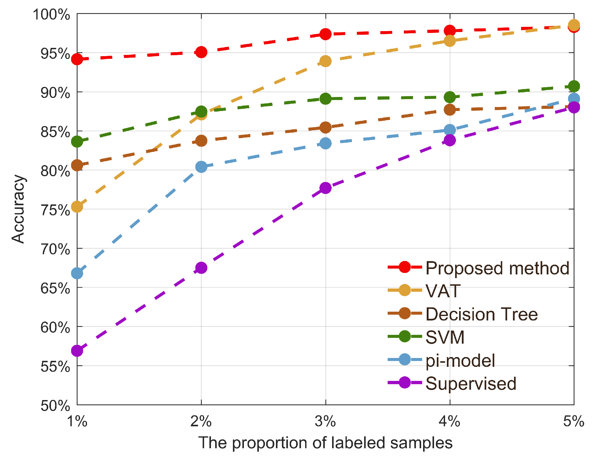
Supervised	0.569	0.596	0.619
Decision Tree	0.806	0.822	0.816
SVM	0.836	0.864	0.863
pi-model	0.668	0.688	0.694
VAT	0.753	0.768	0.772
Proposed method	0.941	0.945	0.939

, our proposed method achieves the best results with a labeled sample proportion of 1–4%. This indicates that semi-supervised learning methods based on pseudo-labeling and consistency regularization perform well in the AMC domain. We find that both semi-supervised learning methods (pi-model, VAT, proposed method) and machine learning methods (decision tree, support vector machine) have a higher classification accuracy than supervised learning methods when the number of labeled samples is small (1–5% of labeled samples). These supervised learning methods only use a backbone network for classification. This suggests that deep-learning-based methods are driven by data, and their classification accuracy is greatly affected in the case of insufficient data samples. The machine-learning-based method is not affected much by the number of data samples. However, it requires hand-designed features, which limits the improvement to the recognition accuracy. We found that the classification accuracy of both semi-supervised learning methods (VAT and Pi-model) is not good when the sample size is extremely small (1% of labeled samples). However, at this point, the recognition accuracy of our proposed semi-supervised method exceeds 94%. This suggests that our proposed method is suitable for scenarios where the number of labeled samples is extremely low. We find that the recognition accuracy of all methods increases as the sample size increases. This is because our proposed method learns the distribution of data not only in unlabelled data but also in labeled data. The greater the amount of labeled data, the more prior knowledge is gained. The recognition performance of the model is improved.

6. Limitations and Future Work

There are two limitations to our work. Related future work is also proposed. Firstly, the purpose of this paper is to demonstrate the efficiency of the proposed semi-supervised approach in automatic modulation classification. Our work has only been validated on one dataset. In practical applications, the data size and class number are not fixed. Therefore, the generalization ability of our proposed method needs further verification. Secondly, our work only classifies known modulation schemes. In practical applications, collected unlabeled signal samples will inevitably include unknown modulation schemes. In future work, we will consider automatic modulation classification in open-set scenarios.

7. Conclusions

In practical automatic modulation classification tasks, the amount of labeled data is very low. To solve this problem, in this paper, we propose a semi-supervised AMC method based on consistency regularization and pseudo-labeling. The proposed method transforms the modulation classification problem into an image classification task. We introduce both strong and weak data augmentation for consistency regularization operations and introduce pseudo-labeling techniques to construct artificial labels. Consistency regularization typically involves two branches handling different perturbations, with a loss function designed to harmonize the predicted outcomes of both branches. Our experimental results show that, compared to five benchmark algorithms, our proposed method achieves a better recognition accuracy when the number of labeled samples is limited. We believe that the proposed approach can help with practical automatic modulation classification tasks.

References

- Zheng, S.; Zhou, X.; Zhang, L.; Qi, P.; Qiu, K.; Zhu, J.; Yang, X. Toward next-generation signal intelligence: A hybrid knowledge and data-driven deep learning framework for radio signal classification. IEEE Trans. Cogn. Commun. Netw. 2023, 9, 564–579. [Google Scholar] [CrossRef]
- Ohtsuki, T. Machine learning in 6G wireless communications. IEICE Trans. Commun. 2023, 106, 75–83. [Google Scholar] [CrossRef]
- Dobre, O.A.; Abdi, A.; Bar-Ness, Y.; Su, W. Survey of automatic modulation classification techniques: Classical approaches and new trends. IET Commun. 2007, 1, 137–156. [Google Scholar] [CrossRef]
- Lin, Y.; Tu, Y.; Dou, Z.; Chen, L.; Mao, S. Contour stella image and deep learning for signal recognition in the physical layer. IEEE Trans. Cogn. Commun. Netw. 2021, 7, 34–46. [Google Scholar] [CrossRef]
- Meng, F.; Chen, P.; Wu, L.; Wang, X. Automatic modulation classification: A deep learning enabled approach. IEEE Trans. Veh. Technol. 2018, 67, 10760–10772. [Google Scholar] [CrossRef]
- Huan, C.; Polydoros, A. Likelihood methods for MPSK modulation classification. IEEE Trans. Commun. 1995, 43, 1493–1504. [Google Scholar] [CrossRef]
- Wei, W.; Mendel, J.M. Maximum-likelihood classification for digital amplitude-phase modulations. IEEE Trans. Commun. 2000, 48, 189–193. [Google Scholar] [CrossRef]
- Hong, L.; Ho, K.C. Antenna array likelihood modulation classifier for BPSK and QPSK signals. In Proceedings of the Military Communications Conference 2002, Anaheim, CA, USA, 7–10 October 2002; pp. 647–651. [Google Scholar]
- Dobre, O.A.; Abdi, A.; Bar-Ness, Y.; Su, W. Selection combining for modulation recognition in fading channels. In Proceedings of the MILCOM 2005–2005 IEEE Military Communications Conference, Atlantic City, NJ, USA, 17–20 October 2005; pp. 2499–2505. [Google Scholar]
- Swami, A.; Sadler, B.M. Hierarchical digital modulation classification using cumulants. IEEE Trans. Commun. 2000, 48, 416–429. [Google Scholar] [CrossRef]
- Ho, K.C.; Prokopiw, W.; Chan, Y.T. Modulation identification by the wavelet transform. In Proceedings of the Military Communications Conference 1995, San Diego, CA, USA, 5–8 November 1995; pp. 886–890. [Google Scholar]
- Chan, Y.T.; Gadbois, L.G. Identification of the modulation type of a signal. Signal Process. 1989, 16, 149–154. [Google Scholar] [CrossRef]
- Xie, L.; Wan, Q. Cyclic Feature-Based Modulation Recognition Using Compressive Sensing. IEEE Wirel. Commun. Lett. 2017, 6, 402–405. [Google Scholar] [CrossRef]
- Wu, H.-C.; Saquib, M.; Yun, Z. Novel Automatic Modulation Classification Using Cumulant Features for Communications via Multipath Channels. IEEE Trans. Wirel. Commun. 2008, 7, 3098–3105. [Google Scholar]
- Peng, S.; Jiang, H.; Wang, H.; Alwageed, H.; Zhou, Y.; Sebdani, M.M.; Yao, Y.D. Modulation Classification Based on Signal Constellation Diagrams and Deep Learning. IEEE Trans. Neural Netw. Learn. Syst. 2019, 30, 718–727. [Google Scholar] [CrossRef] [PubMed]
- Park, C.-S.; Choi, J.-H.; Nah, S.-P.; Jang, W.; Kim, D.Y. Automatic Modulation Recognition of Digital Signals using Wavelet Features and SVM. In Proceedings of the 2008 10th International Conference on Advanced Communication Technology, Gangwon, Republic of Korea, 17–20 February 2008; pp. 387–390. [Google Scholar]
- Park, C.-S.; Jang, W.; Nah, S.-P.; Kim, D.Y. Automatic Modulation Recognition using Support Vector Machine in Software Radio Applications. In Proceedings of the 9th International Conference on Advanced Communication Technology, Gangwon, Republic of Korea, 12–14 February 2007; pp. 9–12. [Google Scholar]
- Liu, Y.; Liang, G.; Xu, X.; Li, X. The Methods of Recognition for Common Used M-ary Digital Modulations. In Proceedings of the 2008 4th International Conference on Wireless Communications, Networking and Mobile Computing, Dalian, China, 12–14 October 2008; pp. 1–4. [Google Scholar]
- Zhang, X.L.; Guo, L.; Ben, C.; Peng, Y.; Wang, Y.; Shi, S.; Lin, Y.; Gui, G. A-GCRNN: Attention graph convolution recurrent neural network for multi-band spectrum prediction. IEEE Trans. Veh. Technol. 2023; early access. [Google Scholar] [CrossRef]
- Gui, G.; Tao, M.; Wang, C.; Fu, X.; Wang, Y. Survey of few-shot learning methods for specific emitter identification. J. Nantong Univ. 2023, 22, 1–16. [Google Scholar]
- Yao, Z.; Fu, X.; Guo, L.; Wang, Y.; Lin, Y.; Shi, S.; Gui, G. Few-shot specific emitter identification using asymmetric masked auto-encoder. IEEE Commun. Lett. 2023, 27, 2657–2661. [Google Scholar] [CrossRef]
- Liu, C.; Fu, X.; Wang, Y.; Guo, L.; Liu, Y.; Lin, Y.; Zhao, H.; Gui, G. Overcoming data limitations: A few-shot specific emitter identification method using self-supervised learning and adversarial augmentation. IEEE Trans. Inf. Forensics Secur. 2023, 19, 500–513. [Google Scholar] [CrossRef]
- Zhang, Q.Y.; Wang, Z.D.; Wu, B.Y.; Gui, G. A robust and practical solution to ADS-B security against denial-of-service attacks. IEEE Internet Things J. 2023. [Google Scholar] [CrossRef]
- Peng, Y.; Hou, C.; Zhang, Y.; Lin, Y.; Gui, G.; Gacanin, H.; Mao, S.; Adachi, A. Supervised contrastive learning for RFF identification with limited samples. IEEE Internet Things J. 2023, 10, 17293–17306. [Google Scholar] [CrossRef]
- Zhang, X.; Chen, X.; Wang, Y.; Gui, G.; Adebisi, B.; Sari, H.; Adachi, F. Lightweight automatic modulation classification via progressive differentiable architecture search. IEEE Trans. Cogn. Commun. Netw. 2023, 9, 1519–1530. [Google Scholar] [CrossRef]
- Wang, Y.; Yang, J.; Liu, M.; Gui, G. LightAMC: Lightweight Automatic Modulation Classification via Deep Learning and Compressive Sensing. IEEE Trans. Veh. Technol. 2020, 69, 3491–3495. [Google Scholar] [CrossRef]
- Wang, Y.; Liu, M.; Yang, J.; Gui, G. Data-Driven Deep Learning for Automatic Modulation Recognition in Cognitive Radios. IEEE Trans. Veh. Technol. 2019, 68, 4074–4077. [Google Scholar] [CrossRef]
- Hong, S.; Zhang, Y.; Wang, Y.; Gu, H.; Gui, G.; Sari, H. Deep Learning-Based Signal Modulation Identification in OFDM Systems. IEEE Access 2019, 7, 114631–114638. [Google Scholar] [CrossRef]
- Guo, Y.; Jiang, H.; Wu, J.; Zhou, J. Open set modulation recognition based on dual-channel LSTM model. arXiv 2020, arXiv:2002.12037. [Google Scholar]
- Zhou, Q.; Zhang, R.; Mu, J.; Zhang, H.; Zhang, F.; Jing, X. AMCRN: Few-Shot Learning for Automatic Modulation Classification. IEEE Commun. Lett. 2022, 26, 542–546. [Google Scholar] [CrossRef]
- Patel, M.; Wang, X.; Mao, S. Data augmentation with conditional GAN for automatic modulation classification. In Proceedings of the 2nd ACM Workshop on Wireless Security and Machine Learning, Virtual, 13 July 2020. [Google Scholar]
- Azzouz, E.; Nandi, A.K. Automatic modulation recognition of communication signals. IEEE Trans. Commun. 1998, 46, 431–436. [Google Scholar]
- Han, Y.; Wei, G.; Song, C.; Lai, L. Hierarchical digital modulation recognition based on higher-order cumulants. In Proceedings of the 2012 Second International Conference on Instrumentation, Measurement, Computer, Communication and Control, Harbin, China, 8–10 December 2012; pp. 1645–1648. [Google Scholar]
- Chou, Z.; Jiang, W.; Xiang, C.; Li, M. Modulation recognition based on constellation diagram for M-QAM signals. In Proceedings of the 2013 IEEE 11th International Conference on Electronic Measurement & Instruments, Harbin, China, 16–19 August 2013; pp. 70–74. [Google Scholar]
- Li, S.; Chen, F.; Wang, L. Modulation identification algorithm based on cyclic spectrum characteristics in multipath channel. J. Comput. Appl. 2012, 32, 2123–2127. [Google Scholar] [CrossRef]
- Wang, D.; Zhang, M.; Li, Z.; Li, J.; Fu, M.; Cui, Y.; Chen, X. Modulation Format Recognition and OSNR Estimation Using CNN-Based Deep Learning. IEEE Photon. Technol. Lett. 2017, 29, 1667–1670. [Google Scholar] [CrossRef]
- O’Shea, T.J.; Corgan, J.; Clancy, T.C. Convolutional radio modulation recognition networks. In Engineering Applications of Neural Networks: 17th International Conference, EANN 2016, Aberdeen, UK, 2–5 September 2016; Proceedings 17; Springer International Publishing: Berlin/Heidelberg, Germany, 2016; pp. 213–226. [Google Scholar]
- Rajendran, S.; Meert, W.; Giustiniano, D.; Lenders, V.; Pollin, S. Deep Learning Models for Wireless Signal Classification With Distributed Low-Cost Spectrum Sensors. IEEE Trans. Cogn. Commun. Netw. 2018, 4, 433–445. [Google Scholar] [CrossRef]
- Ali, A.; Yangyu, F.; Liu, S. Automatic modulation classification of digital modulation signals with stacked autoencoders. Digit. Signal Process. 2017, 71, 108–116. [Google Scholar] [CrossRef]
- Tu, Y.; Lin, Y. Deep Neural Network Compression Technique Towards Efficient Digital Signal Modulation Recognition in Edge Device. IEEE Access 2019, 7, 58113–58119. [Google Scholar] [CrossRef]
- Lee, D. Pseudo-label: The simple and efficient semi-supervised learning method for deep neural networks. Workshop Challenges Represent. Learn. ICML 2013, 3, 896. [Google Scholar]
- Tarvainen, A.; Valpola, H. Mean teachers are better role models: Weight-averaged consistency targets improve semi-supervised deep learning results. Adv. Neural Inf. Process. Syst. 2017, 30. Available online: https://proceedings.neurips.cc/paper_files/paper/2017/file/68053af2923e00204c3ca7c6a3150cf7-Paper.pdf (accessed on 18 January 2024).
- Berthelot, D.; Carlini, N.; Goodfellow, I.; Papernot, N.; Oliver, A.; Raffel, C.A. Mixmatch: A holistic approach to semi-supervised learning. Adv. Neural Inf. Process. Syst. 2019, 32, 1–11. [Google Scholar]
- Zhang, Q.; Xu, Z.; Zhang, P. Modulation scheme recognition using convolutional neural network. J. Eng. 2019, 2019, 9075–9078. [Google Scholar] [CrossRef]
- Cubuk, E.D.; Zoph, B.; Shlens, J.; Le, Q.V. RandAugment: Practical automated data augmentation with a reduced search space. In Proceedings of the 2020 IEEE/CVF Conference on Computer Vision and Pattern Recognition Workshops (CVPRW), Seattle, WA, USA, 14–19 June 2020; pp. 3008–3017. [Google Scholar]
- DeVries, T.; Taylor, G.W. Improved regularization of convolutional neural networks with cutout. arXiv 2017, arXiv:1708.04552. [Google Scholar]
- Cubuk, E.D.; Zoph, B.; Mane, D.; Vasudevan, V.; Le, Q.V. Autoaugment: Learning augmentation policies from data. arXiv 2018, arXiv:1805.09501. [Google Scholar]
- Sohn, K.; Berthelot, D.; Carlini, N.; Zhang, Z.; Zhang, H.; Raffel, C.A.; Cubuk, E.D.; Kurakin, A.; Li, C.L. FixMatch: Simplifying semi-supervised learning with consistency and confidence. Adv. Neural Inf. Process. Syst. 2020, 33, 596–608. [Google Scholar]
- Mohammed, A.; Tahir, A. A new optimizer for image classification using wide ResNet (WRN). Acad. J. Nawroz Univ. 2020, 9, 1–13. [Google Scholar] [CrossRef]
- Miyato, T.; Maeda, S.-I.; Koyama, M.; Ishii, S. Virtual Adversarial Training: A Regularization Method for Supervised and Semi-Supervised Learning. IEEE Trans. Pattern Anal. Mach. Intell. 2019, 41, 1979–1993. [Google Scholar] [CrossRef]