
Advanced Hybrid Transformer-CNN Deep Learning Model for Effective Intrusion Detection Systems with Class Imbalance Mitigation Using Resampling Techniques


Abstract
1. Introduction
- Signature-based IDS: This approach involves scrutinizing network traffic or host activity by matching it against a repository of known malicious patterns. While it excels at detecting familiar threats, its efficacy hinges on continuous updates to remain vigilant against evolving attacks. However, its dependence on established signatures renders it less effective in confronting unknown or zero-day threats, as it lacks the capacity to detect new intrusions that fall outside its predefined dataset.
- Anomaly-based IDS: These systems detect threats by recognizing deviations from established behavioral norms, rather than relying on predefined attack signatures. This makes them particularly adept at identifying zero-day attacks that exploit previously undiscovered vulnerabilities. By utilizing machine learning and deep learning algorithms, anomaly-based IDS can analyze extensive datasets, learn patterns of normal system behavior, and detect anomalies with exceptional precision. This method not only enhances adaptability to emerging threats but also minimizes false positives. In our research, we adopted this approach to improve the accuracy and responsiveness of intrusion detection.
- We create a highly efficient intrusion detection system using an advanced hybrid Transformer-CNN model, integrated with techniques such as ADASYN, SMOTE, ENN, and class weights to effectively tackle class imbalance challenges.
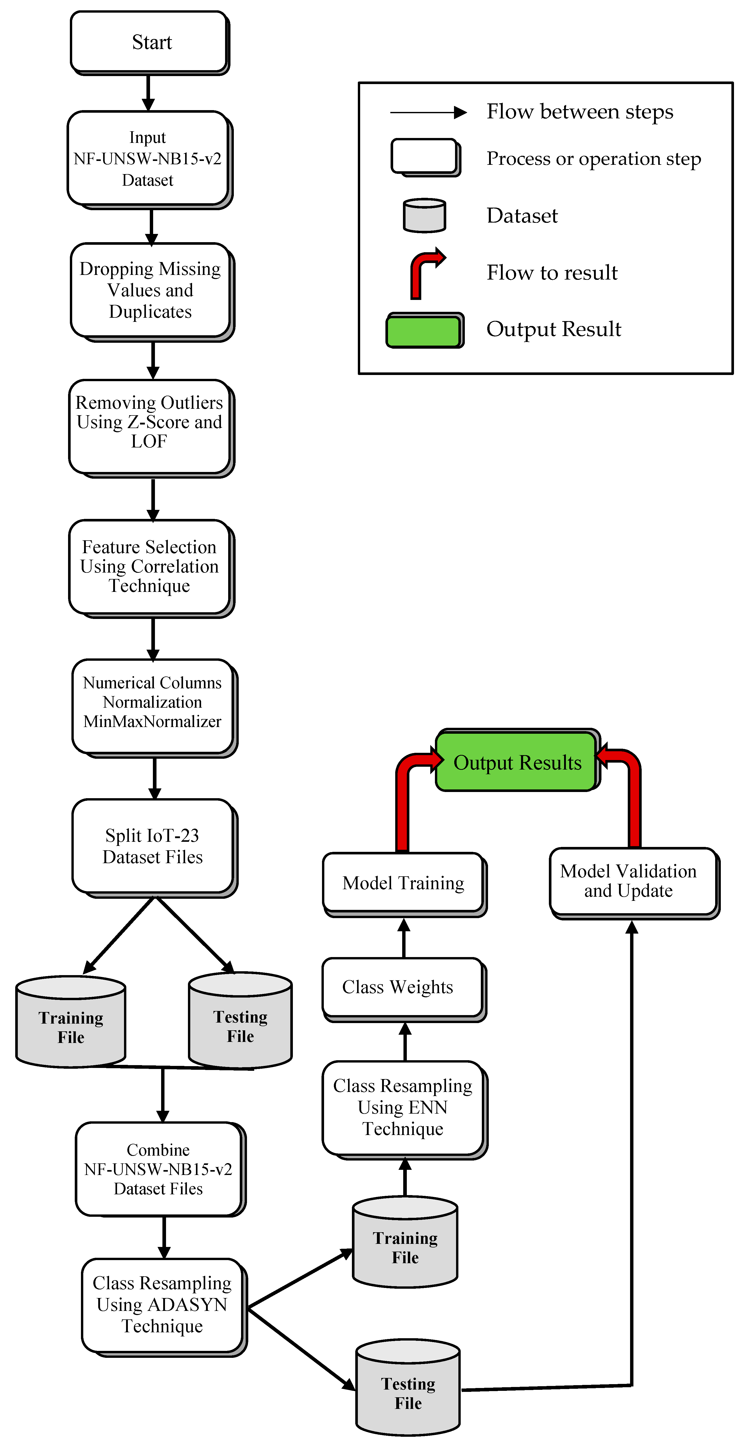
- An enhanced data preprocessing pipeline is applied, which first utilizes a combined outlier detection approach using Z-score and local outlier factor (LOF) to identify and handle outliers, followed by correlation-based feature selection. This structured approach refines model input, enhancing accuracy and reducing computational complexity.
- Using the NF-UNSW-NB15-v2 and CICIDS2017 datasets, this study highlights the exceptional performance of the proposed model, demonstrating its superiority compared to current state-of-the-art models in the field.
2. Related Work
2.1. Binary Classification
2.2. Multi-Class Classification
2.3. Class Imbalances
2.4. Challenges
3. Proposed Approach
3.1. Description of Dataset
3.2. Data Preprocessing
3.2.1. Removing Outliers Using Z-Score and Local Outlier Factor (LOF)
- (i)
- Binary Classification
- (ii)
- Multi-Class Classification
3.2.2. Feature Selection Using Correlation Technique
- (i)
- Binary Classification
- (ii)
- Multi-Class Classification
3.2.3. Normalization
3.2.4. Train-Test Dataset Split
- (i)
- Binary Classification
- (ii)
- Multi-Class Classification
3.2.5. Class Balancing
- ADASYN
- (i)
- Binary Classification
- (ii)
- Multi-Class Classification
- 2.
- ENN
- (i)
- Binary Classification
- (ii)
- Multi-Class Classification
- 3.
- Class Weights
- (i)
- Binary Classification
- (ii)
- Multi-Class Classification
3.3. Architectures of Models
3.3.1. Convolutional Neural Networks (CNN)
- (i)
- Binary Classification
- (ii)
- Multi-Class Classification
- (iii)
- Hyperparameter Configuration for the CNN Model
3.3.2. Auto Encoder (AE)
- (i)
- Binary Classification
- (ii)
- Multi-Class Classification
- (iii)
- Hyperparameter Configuration for the Auto Encoder Model
3.3.3. Deep Neural Network (DNN)
- (i)
- Binary Classification
- (ii)
- Multi-Class Classification
- (iii)
- Hyperparameter Configuration for the DNN Model
3.3.4. Transformer-Convolutional Neural Network (Transformer CNN)
- (i)
- Binary Classification
- (ii)
- Multi-Class Classification
- (iii)
- Hyperparameter Configuration for the Transformer-CNN Model
4. Results and Experiments
4.1. Dataset Description and Preprocessing Overview
4.1.1. NF-UNSW-NB15-v2 Dataset
4.1.2. CICIDS2017 Dataset
4.2. Experiment’s Establishment
4.3. Evaluation Metrics
- True Positive (TP): These are the instances that the model correctly predicted to be positive. For example, if a spam filter correctly identified an email as spam, this is a true positive.
- False Negative (FN): These are the instances that the model incorrectly predicted to be negative. In the spam filter example, if it mistakenly classified a spam email as legitimate, this is a false negative.
- True Negative (TN): These are the instances that the model correctly predicted to be negative. Returning to our spam filter, if it accurately identified a non-spam email as non-spam, this is a true negative.
- False Positive (FP): These are the instances that the model incorrectly predicted to be positive. In the spam filter context, if it mistakenly classified a legitimate email as spam, this is a false positive.
4.4. Results
- (i)
- Binary Classification
- (ii)
- Multi-Class Classification
5. Discussion
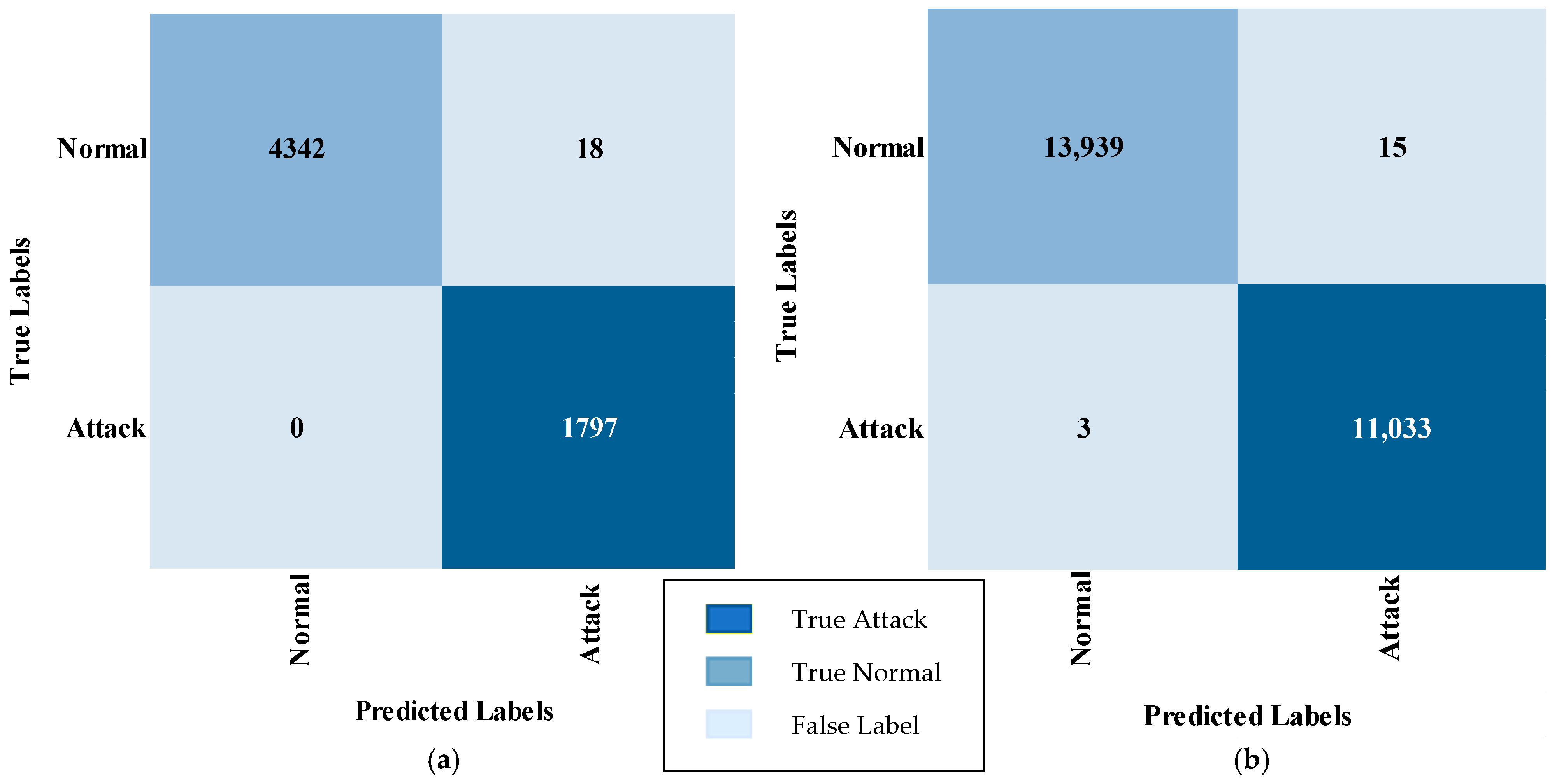
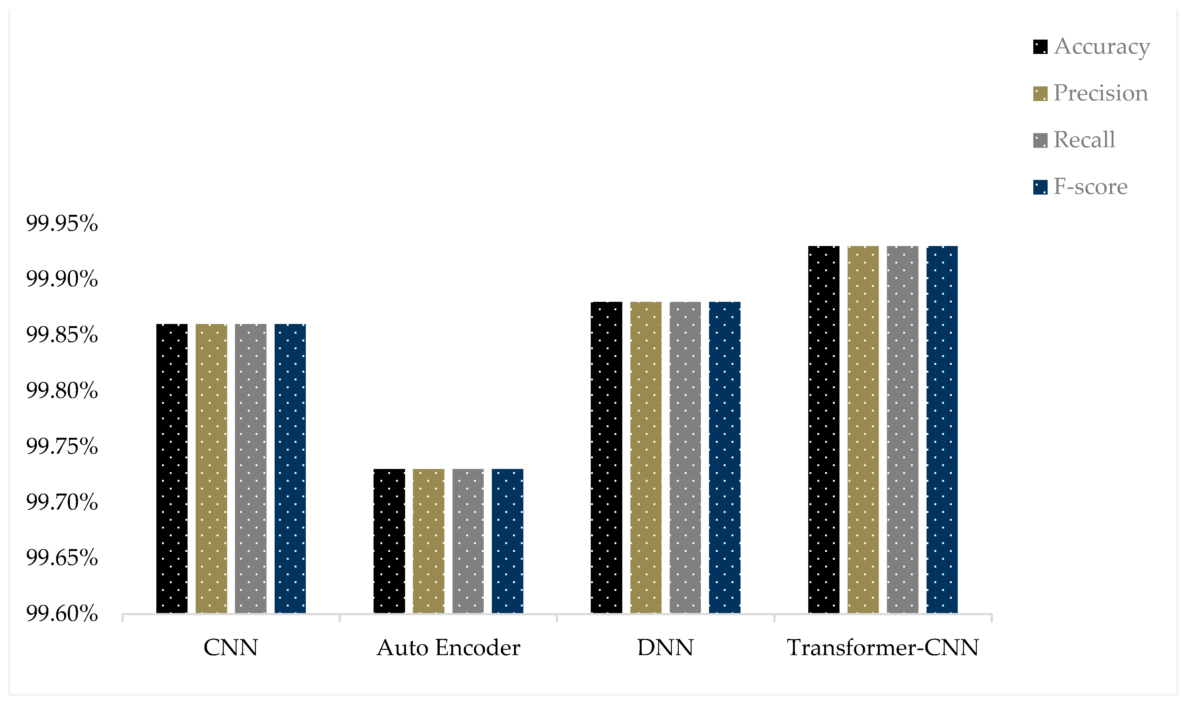
- (i)
- Binary Classification
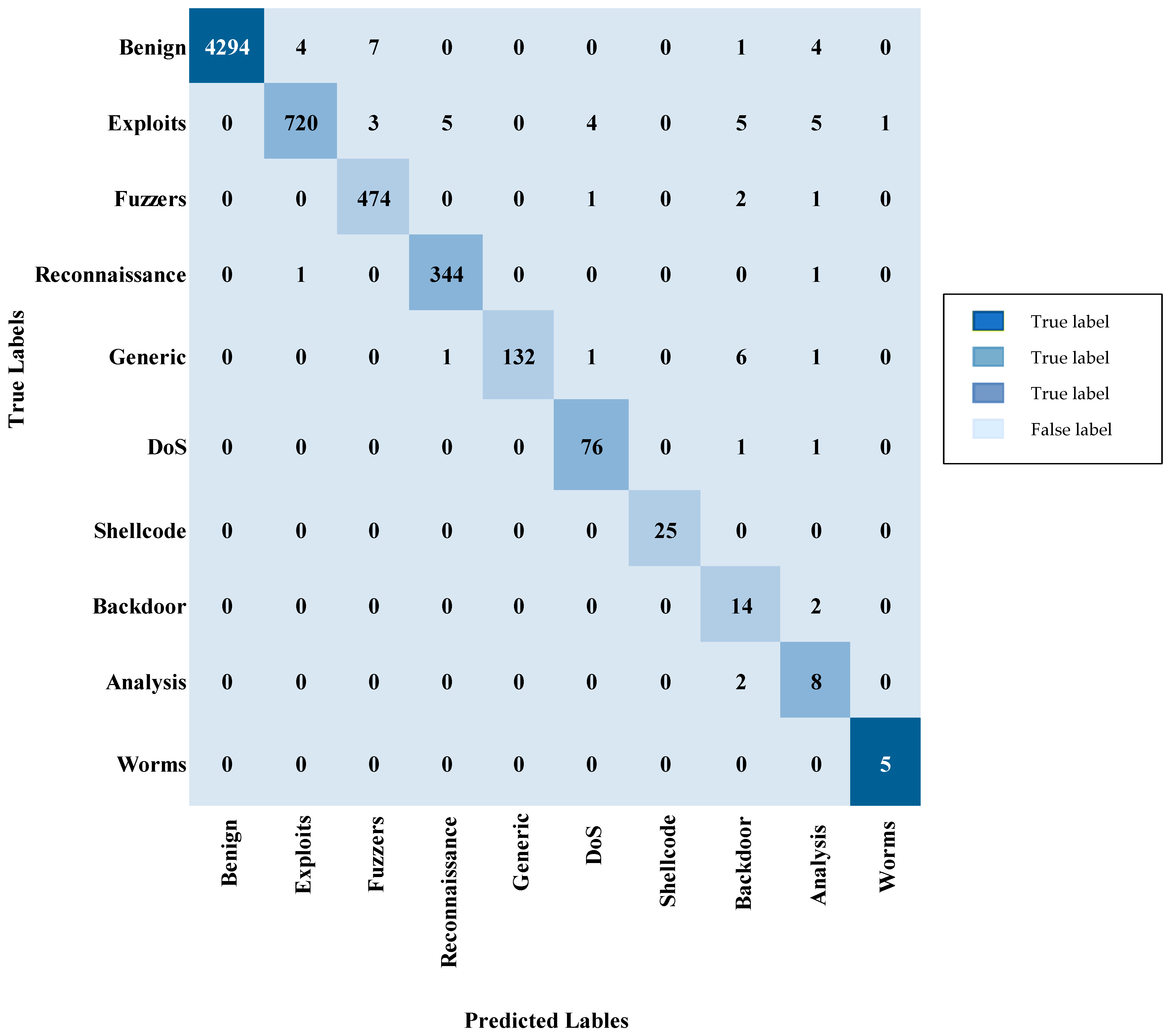
- (ii)
- Multi-Class Classification
Case Study for Zero-Day Attack
6. Limitations
- Scalability: As the volume of datasets or the complexity of network traffic grows, the computational demands on the model can intensify, which may hinder its efficiency and its capacity to manage larger datasets or adapt to changing network environments.
- Generalization: Although the Transformer-CNN exhibits impressive performance on the NF-UNSW-NB15-v2 and CICIDS2017 datasets, its efficacy across diverse types of network traffic or newly emerging attack vectors is not yet fully established. To assess its robustness and generalization capabilities, it is crucial to evaluate the model against a wider array of datasets, including KDDCup99 [36], NSL KDD [29], and more recent collections like CSE-CIC-IDS2018 [34], and IoT23 [16].
- Data Preprocessing: The execution of data preprocessing across various datasets is a vital stage that encompasses activities like addressing missing values, encoding categorical variables, normalizing or standardizing numerical features, and eliminating extraneous information. The model’s performance is significantly influenced by the quality and thoroughness of these preprocessing procedures.
- Model Adaptation: Adjusting the model for various datasets necessitates a trial-and-error approach to hyperparameter optimization. This iterative process is essential for refining the model to better match the specific characteristics and nuances of new datasets.
7. Conclusions
8. Future Work
- Broader Dataset Evaluation: Future investigations should involve testing the Transformer-CNN across a more diverse range of datasets, including KDDCup99 [36], NSL KDD [29], and newer datasets such as CSE-CIC-IDS2018 [34], and IoT23 [16]. This approach will provide insights into its robustness, generalization potential, and effectiveness in addressing emerging attack vectors.
- Data Preprocessing Refinement: The data preprocessing procedures should be meticulously refined and customized for each dataset to achieve optimal model performance. This entails experimenting with various preprocessing techniques and analyzing their effects on model results. Comprehensive discussions of these preprocessing strategies are extensively covered in Section 3.2 and 4.1 of the manuscript.
- Model Adaptation and Hyperparameter Optimization: Ongoing investigation into model adaptation techniques is essential, emphasizing the refinement of the hyperparameter optimization process tailored to various datasets. This process should undergo systematic analysis to uncover best practices for effectively adapting the model to different data environments. Detailed discussions of these aspects are presented in Section 3, specifically in Section 3.3.4.
- Scalability and Computational Efficiency: It is imperative to enhance the model’s computational efficiency and scalability, enabling it to effectively manage larger datasets and more intricate network traffic scenarios without sacrificing performance.
Author Contributions
Funding
Data Availability Statement
Conflicts of Interest
References
- Conti, M.; Dargahi, T.; Dehghantanha, A. Cyber Threat Intelligence: Challenges and Opportunities; Springer: Berlin/Heidelberg, Germany, 2018; pp. 1–6. [Google Scholar] [CrossRef]
- Faker, O.; Dogdu, E. Intrusion detection using big data and deep learning techniques. In Proceedings of the 2019 ACM Southeast Conference. ACM SE’19, Kennesaw, GA, USA, 18–20 April 2019; Association for Computing Machinery: New York, NY, USA, 2019; pp. 86–93. [Google Scholar] [CrossRef]
- Kaur, G.; Habibi Lashkari, A.; Rahali, A. Intrusion trafc detection and characterization using deep image learning. In Proceedings of the 2020 IEEE International Conference on Dependable, Autonomic and Secure Computing, International Conference on Pervasive Intelligence and Computing, International Conference on Cloud and Big Data Computing, Intl Conf on Cyber Science and Technology Congress (DASC/PiCom/CBDCom/CyberSciTech), Calgary, AB, Canada, 17–22 August 2020; pp. 55–62. [Google Scholar] [CrossRef]
- Internet Security Threat Report. Available online: https://docs.broadcom.com/doc/istr-23-2018-en (accessed on 18 July 2022).
- Cyberattacks Now Cost Companies \$200,000 on Average, Putting Many out of Business. Available online: https://www.cnbc.com/2019/10/13/cyberattacks-cost-small-companies-200k-putting-many-out-of-business.html (accessed on 13 October 2019).
- Kumar, M.; Singh, A.K. Distributed intrusion detection system using blockchain and cloud computing infrastructure. In Proceedings of the 2020 4th International Conference on Trends in Electronics and Informatics (ICOEI)(48184), Tirunelveli, India, 15–17 June 2020; pp. 248–252. [Google Scholar]
- Zhang, X.; Xie, J.; Huang, L. Real-Time Intrusion Detection Using Deep Learning Techniques. J. Netw. Comput. Appl. 2020, 140, 45–53. [Google Scholar]
- Kumar, S.; Kumar, R. A Review of Real-Time Intrusion Detection Systems Using Machine Learning Approaches. Comput. Secur. 2020, 95, 101944. [Google Scholar]
- Smith, A.; Jones, B.; Taylor, C. Enhancing Network Security with Real-Time Intrusion Detection Systems. Int. J. Inf. Secur. 2021, 21, 123–135. [Google Scholar]
- Sarhan, M.; Layeghy, S.; Portmann, M. Towards a standard feature set for network intrusion detection system datasets. Mob. Netw. Appl. 2022, 27, 357–370. [Google Scholar] [CrossRef]
- Sarhan, M.; Layeghy, S.; Moustafa, N.; Portmann, M. Cyber threat intelligence sharing scheme based on federated learning for network intrusion detection. J. Netw. Syst. Manag. 2023, 31, 3. [Google Scholar] [CrossRef]
- UNB. Intrusion Detection Evaluation Dataset (CICIDS2017), University of New Brunswick. Available online: https://www.unb.ca/cic/datasets/ids-2017.html (accessed on 30 October 2024).
- Panigrahi, R.; Borah, S. A detailed analysis of CICIDS2017 dataset for designing Intrusion Detection Systems. Int. J. Eng. Technol. 2018, 7, 479–482. [Google Scholar]
- Anderson, J.P. Computer security threat monitoring and surveillance. In Technical Report; James P. Anderson Company: Washington, DC, USA, 1980. [Google Scholar]
- Mahalingam, A.; Perumal, G.; Subburayalu, G.; Albathan, M.; Altameem, A.; Almakki, R.S.; Hussain, A.; Abbas, Q. ROAST-IoT: A novel range-optimized attention convolutional scattered technique for intrusion detection in IoT networks. Sensors 2023, 23, 8044. [Google Scholar] [CrossRef]
- ElKashlan, M.; Elsayed, M.S.; Jurcut, A.D.; Azer, M. A machine learning-based intrusion detection system for iot electric vehicle charging stations (evcss). Electronics 2023, 12, 1044. [Google Scholar] [CrossRef]
- Al Nuaimi, T.; Al Zaabi, S.; Alyilieli, M.; AlMaskari, M.; Alblooshi, S.; Alhabsi, F.; Yusof, M.F.B.; Al Badawi, A. A comparative evaluation of intrusion detection systems on the edge-IIoT-2022 dataset. Intell. Syst. Appl. 2023, 20, 200298. [Google Scholar] [CrossRef]
- Gad, A.R.; Nashat, A.A.; Barkat, T.M. Intrusion detection system using machine learning for vehicular ad hoc networks based on ToN-IoT dataset. IEEE Access 2021, 9, 142206–142217. [Google Scholar] [CrossRef]
- Al-Daweri, M.S.; Ariffin, K.A.Z.; Abdullah, S.; Senan, M.F.E.M. An analysis of the KDD99 and UNSW-NB15 datasets for the intrusion detection system. Symmetry 2020, 12, 1666. [Google Scholar] [CrossRef]
- Vitorino, J.; Praça, I.; Maia, E. Towards adversarial realism and robust learning for IoT intrusion detection and classification. Ann. Telecommun. 2023, 78, 401–412. [Google Scholar] [CrossRef]
- Othman, T.S.; Abdullah, S.M. An intelligent intrusion detection system for internet of things attack detection and identification using machine learning. Aro-Sci. J. Koya Univ. 2023, 11, 126–137. [Google Scholar] [CrossRef]
- Yaras, S.; Dener, M. IoT-Based Intrusion Detection System Using New Hybrid Deep Learning Algorithm. Electronics 2024, 13, 1053. [Google Scholar] [CrossRef]
- Vinayakumar, R.; Alazab, M.; Soman, K.P.; Poornachandran, P.; Al-Nemrat, A.; Venkatraman, S. Deep learning approach for intelligent intrusion detection system. IEEE Access 2019, 7, 41525–41550. [Google Scholar] [CrossRef]
- Farhana, K.; Rahman, M.; Ahmed, M.T. An intrusion detection system for packet and flow based networks using deep neural network approach. Int. J. Electr. Comput. Eng. 2020, 10, 5514–5525. [Google Scholar] [CrossRef]
- Zhang, C.; Chen, Y.; Meng, Y.; Ruan, F.; Chen, R.; Li, Y.; Yang, Y. A novel framework design of network intrusion detection based on machine learning techniques. Secur. Commun. Netw. 2021, 2021, 6610675. [Google Scholar] [CrossRef]
- Alsharaiah, M.; Abualhaj, M.; Baniata, L.; Al-saaidah, A.; Kharma, Q.; Al-Zyoud, M. An innovative network intrusion detection system (NIDS): Hierarchical deep learning model based on Unsw-Nb15 dataset. Int. J. Data Netw. Sci. 2024, 8, 709–722. [Google Scholar] [CrossRef]
- Jouhari, M.; Benaddi, H.; Ibrahimi, K. Efficient Intrusion Detection: Combining χ2 Feature Selection with CNN-BiLSTM on the UNSW-NB15 Dataset. arXiv 2024, arXiv:2407.14945. [Google Scholar]
- Türk, F. Analysis of intrusion detection systems in UNSW-NB15 and NSL-KDD datasets with machine learning algorithms. Bitlis Eren Üniversitesi Fen Bilim. Derg. 2023, 12, 465–477. [Google Scholar] [CrossRef]
- Muhuri, P.; Chatterjee, P.; Yuan, X.; Roy, K.; Esterline, A. Using a long short-term memory recurrent neural network (lstm-rnn) to classify network attacks. Information 2020, 11, 243. [Google Scholar] [CrossRef]
- Fu, Y.; Du, Y.; Cao, Z.; Li, Q.; Xiang, W. A deep learning model for network intrusion detection with imbalanced data. Elec-tronics 2022, 11, 898. [Google Scholar] [CrossRef]
- Yin, Y.; Jang-Jaccard, J.; Xu, W.; Singh, A.; Zhu, J.; Sabrina, F.; Kwak, J. IGRF-RFE: A hybrid feature selection method for MLP-based network intrusion detection on UNSW-NB15 dataset. J. Big Data 2023, 10, 15. [Google Scholar] [CrossRef]
- Yoo, J.; Min, B.; Kim, S.; Shin, D.; Shin, D. Study on network intrusion detection method using discrete pre-processing method and convolution neural network. IEEE Access 2021, 9, 142348–142361. [Google Scholar] [CrossRef]
- Alzughaibi, S.; El Khediri, S. A cloud intrusion detection systems based on dnn using backpropagation and pso on the cse-cic-ids2018 dataset. Appl. Sci. 2023, 13, 2276. [Google Scholar] [CrossRef]
- Basnet, R.B.; Shash, R.; Johnson, C.; Walgren, L.; Doleck, T. Towards Detecting and Classifying Network Intrusion Traffic Using Deep Learning Frameworks. J. Internet Serv. Inf. Secur. 2019, 9, 1–17. [Google Scholar]
- Thilagam, T.; Aruna, R. Intrusion detection for network based cloud computing by custom RC-NN and optimization. ICT Express 2021, 7, 512–520. [Google Scholar] [CrossRef]
- Farahnakian, F.; Heikkonen, J. A deep auto-encoder based approach for intrusion detection system. In Proceedings of the 2018 20th International Conference on Advanced Communication Technology (ICACT), Chuncheon, Republic of Korea, 11–14 February 2018; IEEE: Piscataway, NJ, USA, 2018; pp. 178–183. [Google Scholar]
- Mahmood, H.A.; Hashem, S.H. Network intrusion detection system (NIDS) in cloud environment based on hid-den Naïve Bayes multiclass classifier. Al-Mustansiriyah J. Sci. 2018, 28, 134–142. [Google Scholar] [CrossRef]
- Baig, M.M.; Awais, M.M.; El-Alfy, E.S.M. A multiclass cascade of artificial neural network for network intrusion detection. J. Intell. Fuzzy Syst. 2017, 32, 2875–2883. [Google Scholar] [CrossRef]
- Mohy-Eddine, M.; Guezzaz, A.; Benkirane, S.; Azrour, M.; Farhaoui, Y. An ensemble learning based intrusion detection model for industrial IoT security. Big Data Min. Anal. 2023, 6, 273–287. [Google Scholar] [CrossRef]
- Nicolas-Alin, S. Machine Learning for Anomaly Detection in Iot Networks: Malware Analysis on the Iot-23 Data Set. Bachelor’s Thesis, University of Twente, Enschede, The Netherland, 2020. [Google Scholar]
- Susilo, B.; Sari, R.F. Intrusion detection in IoT networks using deep learning algorithm. Information 2020, 11, 279. [Google Scholar] [CrossRef]
- Szczepański, M.; Pawlicki, M.; Kozik, R.; Choraś, M. The application of deep learning imputation and other advanced methods for handling missing values in network intrusion detection. Vietnam. J. Comput. Sci. 2023, 10, 1–23. [Google Scholar] [CrossRef]
- Kumar, P.; Bagga, H.; Netam, B.S.; Uduthalapally, V. Sad-iot: Security analysis of ddos attacks in iot networks. Wirel. Pers. Commun. 2022, 122, 87–108. [Google Scholar] [CrossRef]
- Sarhan, M.; Layeghy, S.; Portmann, M. Feature analysis for machine learning-based IoT intrusion detection. arXiv 2021, arXiv:2108.12732. [Google Scholar]
- Ferrag, M.A.; Friha, O.; Hamouda, D.; Maglaras, L.; Janicke, H. Edge-IIoTset: A new comprehensive realistic cyber security dataset of IoT and IIoT applications for centralized and federated learning. IEEE Access 2022, 10, 40281–40306. [Google Scholar] [CrossRef]
- Henry, A.; Gautam, S.; Khanna, S.; Rabie, K.; Shongwe, T.; Bhattacharya, P.; Sharma, B.; Chowdhury, S. Composition of hybrid deep learning model and feature optimization for intrusion detection system. Sensors 2023, 23, 890. [Google Scholar] [CrossRef] [PubMed]
- Aleesa, A.; Mohammed, A.A.; Mohammed, A.A.; Sahar, N. Deep-intrusion detection system with enhanced UNSW-NB15 dataset based on deep learning techniques. J. Eng. Sci. Technol. 2021, 16, 711–727. [Google Scholar]
- Ahmad, M.; Riaz, Q.; Zeeshan, M.; Tahir, H.; Haider, S.A.; Khan, M.S. Intrusion detection in internet of things using supervised machine learning based on application and transport layer features using UNSW-NB15 data-set. EURASIP J. Wirel. Commun. Netw. 2021, 2021, 10. [Google Scholar] [CrossRef]
- Mohammed, B.; Gbashi, E.K. Intrusion detection system for NSL-KDD dataset based on deep learning and recursive feature elimination. Eng. Technol. J. 2021, 39, 1069–1079. [Google Scholar] [CrossRef]
- Umair, M.B.; Iqbal, Z.; Faraz, M.A.; Khan, M.A.; Zhang, Y.D.; Razmjooy, N.; Kadry, S. A network intrusion detection system using hybrid multilayer deep learning model. Big Data 2022, 12, 367–376. [Google Scholar] [CrossRef]
- Choobdar, P.; Naderan, M.; Naderan, M. Detection and multi-class classification of intrusion in software defined networks using stacked auto-encoders and CICIDS2017 dataset. Wirel. Pers. Commun. 2022, 123, 437–471. [Google Scholar] [CrossRef]
- Shende, S.; Thorat, S. Long short-term memory (LSTM) deep learning method for intrusion detection in network security. Int. J. Eng. Res. 2020, 9, 1615–1620. [Google Scholar]
- Farhan, B.I.; Jasim, A.D. Performance analysis of intrusion detection for deep learning model based on CSE-CIC-IDS2018 dataset. Indones. J. Electr. Eng. Comput. Sci. 2022, 26, 1165–1172. [Google Scholar] [CrossRef]
- Farhan, R.I.; Maolood, A.T.; Hassan, N. Performance analysis of flow-based attacks detection on CSE-CIC-IDS2018 dataset using deep learning. Indones. J. Electr. Eng. Comput. Sci. 2020, 20, 1413–1418. [Google Scholar] [CrossRef]
- Lin, P.; Ye, K.; Xu, C.Z. Dynamic network anomaly detection system by using deep learning techniques. In Proceedings of the Cloud Computing–CLOUD 2019: 12th International Conference, Held as Part of the Services Conference Federation, SCF 2019, San Diego, CA, USA, 25–30 June 2019; Proceedings 12. Springer International Publishing: Berlin/Heidelberg, Germany, 2019; pp. 161–176. [Google Scholar]
- Liu, G.; Zhang, J. CNID: Research of network intrusion detection based on convolutional neural network. Discret. Dyn. Nat. Soc. 2020, 2020, 4705982. [Google Scholar] [CrossRef]
- Li, F.; Shen, H.; Mai, J.; Wang, T.; Dai, Y.; Miao, X. Pre-trained language model-enhanced conditional generative adversarial networks for intrusion detection. Peer-to-Peer Netw. Appl. 2024, 17, 227–245. [Google Scholar] [CrossRef]
- Wang, S.; Yao, X. Multiclass imbalance problems: Analysis and potential solutions. IEEE Trans. Syst. Man Cybern. Part B 2012, 42, 1119–1130. [Google Scholar] [CrossRef] [PubMed]
- Abdelkhalek, A.; Mashaly, M. Addressing the class imbalance problem in network intrusion detection systems using data resampling and deep learning. J. Supercomput. 2023, 79, 10611–10644. [Google Scholar] [CrossRef]
- Yang, H.; Xu, J.; Xiao, Y.; Hu, L. SPE-ACGAN: A resampling approach for class imbalance problem in network intrusion detection systems. Electronics 2023, 12, 3323. [Google Scholar] [CrossRef]
- Zakariah, M.; AlQahtani, S.A.; Al-Rakhami, M.S. Machine learning-based adaptive synthetic sampling technique for intrusion detection. Appl. Sci. 2023, 13, 6504. [Google Scholar] [CrossRef]
- Thiyam, B.; Dey, S. Efficient feature evaluation approach for a class-imbalanced dataset using machine learning. Procedia Comput. Sci. 2023, 218, 2520–2532. [Google Scholar] [CrossRef]
- AlbAlbasheer, F.O.; Haibatti, R.R.; Agarwal, M.; Nam, S.Y. A Novel IDS Based on Jaya Optimizer and Smote-ENN for Cyberattacks Detection. IEEE Access 2024, 12, 101506–101527. [Google Scholar] [CrossRef]
- Arık, A.O.; Çavdaroğlu, G.Ç. An Intrusion Detection Approach based on the Combination of Oversampling and Undersampling Algorithms. Acta Infologica 2023, 7, 125–138. [Google Scholar] [CrossRef]
- Rao, Y.N.; Suresh Babu, K. An imbalanced generative adversarial network-based approach for network intrusion detection in an imbalanced dataset. Sensors 2023, 23, 550. [Google Scholar] [CrossRef]
- Jamoos, M.; Mora, A.M.; AlKhanafseh, M.; Surakhi, O. A new data-balancing approach based on generative adversarial network for network intrusion detection system. Electronics 2023, 12, 2851. [Google Scholar] [CrossRef]
- Xu, B.; Sun, L.; Mao, X.; Ding, R.; Liu, C. IoT Intrusion Detection System Based on Machine Learning. Electronics 2023, 12, 4289. [Google Scholar] [CrossRef]
- Assy, A.T.; Mostafa, Y.; Abd El-khaleq, A.; Mashaly, M. Anomaly-based intrusion detection system using one-dimensional convolutional neural network. Procedia Comput. Sci. 2023, 220, 78–85. [Google Scholar] [CrossRef]
- Elghalhoud, O.; Naik, K.; Zaman, M.; Manzano, R. Data Balancing and cnn Based Network Intrusion Detection System; IEEE: Piscataway, NJ, USA, 2023. [Google Scholar]
- Almarshdi, R.; Nassef, L.; Fadel, E.; Alowidi, N. Hybrid Deep Learning Based Attack Detection for Imbalanced Data Classification. Intell. Autom. Soft Comput. 2023, 35, 297–320. [Google Scholar] [CrossRef]
- Thockchom, N.; Singh, M.M.; Nandi, U. A novel ensemble learning-based model for network intrusion detection. Complex Intell. Syst. 2023, 9, 5693–5714. [Google Scholar] [CrossRef]
- Jumabek, A.; Yang, S.S.; Noh, Y.T. CatBoost-based network intrusion detection on imbalanced CIC-IDS-2018 dataset. Korean Soc. Commun. Commun. J. 2021, 46, 2191–2197. [Google Scholar] [CrossRef]
- Zhu, Y.; Liang, J.; Chen, J.; Ming, Z. An improved nsga-iii algorithm for feature selection used in intrusion detection. Knowl.-Based Syst. 2017, 116, 74–85. [Google Scholar] [CrossRef]
- Jiang, J.; Wang, Q.; Shi, Z.; Lv, B.; Qi, B. Rst-rf: A hybrid model based on rough set theory and random forest for network intrusion detection. In Proceedings of the 2nd International Conference on Cryptography, Security and Privacy, Guiyang, China, 16–18 March 2018. [Google Scholar]
- Chawla, N.; Bowyer, K.; Hall, L.; Kegelmeyer, W. Smote: Synthetic minority over-sampling technique. J. Artif. Intell. Res. 2002, 16, 321–357. [Google Scholar] [CrossRef]
- Alikhanov, J.; Jang, R.; Abuhamad, M.; Mohaisen, D.; Nyang, D.; Noh, Y. Investigating the effect of trafc sampling on machine learning-based network intrusion detection approaches. IEEE Access 2022, 10, 5801–5823. [Google Scholar] [CrossRef]
- Zhang, X.; Ran, J.; Mi, J. An intrusion detection system based on convolutional neural network for imbalanced network trafc. In Proceedings of the 2019 IEEE 7th International Conference on Computer Science and Network Technology (ICCSNT), Dalian, China, 19–20 October 2019; pp. 456–460. [Google Scholar]
- Gupta, N.; Jindal, V.; Bedi, P. CSE-IDS: Using cost-sensitive deep learning and ensemble algorithms to handle class imbalance in Network-based intrusion detection systems. Comput. Secur. 2021, 112, 102499. [Google Scholar] [CrossRef]
- Mbow, M.; Koide, H.; Sakurai, K. Handling class imbalance problem in intrusion detection system based on deep learning. Int. J. Netw. Comput. 2022, 12, 467–492. [Google Scholar] [CrossRef] [PubMed]
- Patro, S.G.; Sahu, D.-K.K. Normalization: A preprocessing stage. arXiv 2015, arXiv:1503.06462. [Google Scholar] [CrossRef]
- Bagui, S.; Li, K. Resampling imbalanced data for network intrusion detection datasets. J. Big Data 2021, 8, 6. [Google Scholar] [CrossRef]
- Elmasry, W.; Akbulut, A.; Zaim, A.H. Empirical study on multiclass classifcation-based network intrusion detection. Comput. Intell. 2019, 35, 919–954. [Google Scholar] [CrossRef]
- El-Habil, B.Y.; Abu-Naser, S.S. Global climate prediction using deep learning. J. Theor. Appl. Inf. Technol. 2022, 100, 4824–4838. [Google Scholar]
- He, H.; Wu, D. ADASYN: Adaptive Synthetic Sampling Approach for Imbalanced Learning. In Proceedings of the 2008 Fourth International Conference on Natural Computation, Jinan, China, 18–20 October 2008. [Google Scholar]
- Wilson, D.L. Asymptotic properties of nearest neighbor rules using edited data. IEEE Trans. Syst. Man Cybern. 1972, 3, 408–421. [Google Scholar] [CrossRef]
- He, H.; Garcia, E. Learning from imbalanced data. In IEEE Transactions on Knowledge and Data Engineering; IEEE: Piscataway, NJ, USA, 2009. [Google Scholar]
- Zhendong, S.; Jinping, M. Deep learning-driven MIMO: Data encoding and processing mechanism. Phys. Commun. 2022, 57, 101976. [Google Scholar] [CrossRef]
- Xin, Z.; Chunjiang, Z.; Jun, S.; Kunshan, Y.; Min, X. Detection of lead content in oilseed rape leaves and roots based on deep transfer learning and hyperspectral imaging technology. Spectrochim. Acta Part A Mol. Biomol. Spectrosc. 2022, 290, 122288. [Google Scholar] [CrossRef]
- Goodfellow, I.; Bengio, Y.; Courville, A. Deep Learning; MIT Press: Cambridge, MA, USA, 2016. [Google Scholar]
- Nair, V.; Hinton, G.E. Rectified linear units improve restricted boltzmann machines. In Proceedings of the 27th International Conference on Machine Learning (ICML-10), Haifa, Israel, 21–24 June 2010; pp. 807–814. [Google Scholar]
- Srivastava, N.; Hinton, G.; Krizhevsky, A.; Sutskever, I.; Salakhutdinov, R. Dropout: A simple way to prevent neural networks from overfitting. J. Mach. Learn. Res. 2014, 15, 1929–1958. [Google Scholar]
- Bishop, C.M.; Nasrabadi, N.M. Pattern Recognition And Machine Learning; Springer: New York, MY, USA, 2006; Volume 4. [Google Scholar]
- Nielsen, M.A. Neural Networks and Deep Learning. In Chapter 1 Explains the Basics of Feedforward Operations in Neural Networks; Determination Press: San Francisco, CA, USA, 2015. [Google Scholar]
- Glorot, X.; Bordes, A.; Bengio, Y. Deep Sparse Rectifier Neural Networks. In Proceedings of the Fourteenth International Conference on Artificial Intelligence and Statistics, Fort Lauderdale, FL, USA, 11–13 April 2011. [Google Scholar]
- Vaswani, A.; Noam, S.; Niki, P.; Jakob, U.; Llion, J.; Aidan, N.G.; Lukasz, K.; Illia, P. Attention Is All You Need.(Nips), 2017. arXiv 2017, arXiv:1706.03762. [Google Scholar]
- Lei Ba, J.; Kiros, J.R.; Hinton, G.E. Layer normalization. arXiv 2016, arXiv:1607.06450. [Google Scholar]
- Ring, M.; Wunderlich, S.; Scheuring, D.; Landes, D.; Hotho, A. A survey of network-based intrusion detection data sets. Comput. Secur. 2019, 86, 147–167. [Google Scholar] [CrossRef]
- Sharafaldin, I.; Lashkari, A.H.; Ghorbani, A.A. Toward generating a new intrusion detection dataset and intrusion traffic characterization. ICISSp 2018, 1, 108–116. [Google Scholar]
- Sharafaldin, I.; Habibi Lashkari, A.; Ghorbani, A.A. A detailed analysis of the cicids2017 data set. In Proceedings of the Information Systems Security and Privacy: 4th International Conference, ICISSP 2018, Funchal-Madeira, Portugal, 22–24 January 2018; Revised Selected Papers 4. Springer International Publishing: Berlin/Heidelberg, Germany, 2019; pp. 172–188. [Google Scholar]
- Jyothsna, V.; Prasad, K.M. Anomaly-based intrusion detection system. In Computer and Network Security; Intech: Houston, TX, USA, 2019; Volume 10. [Google Scholar]
- Chen, C.; Song, Y.; Yue, S.; Xu, X.; Zhou, L.; Lv, Q.; Yang, L. FCNN-SE: An Intrusion Detection Model Based on a Fusion CNN and Stacked Ensemble. Appl. Sci. 2022, 12, 8601. [Google Scholar] [CrossRef]
- Powers, D.M.W. Evaluation: From Precision, Recall, and F-Measure to ROC, Informedness, Markedness & Correlation. J. Mach. Learn. Technol. 2011, 2, 37–63. [Google Scholar]


| Author | Dataset | Year | Utilized Technique | Accuracy | Contribution | Limitations |
|---|---|---|---|---|---|---|
| Anandaraj Mahalingam et al. [15] | IoT-23 | 2023 | ROAST-IoT | 99.15% | This paper introduces ROAST-IoT, an AI-based model designed for efficient intrusion detection in IoT environments. It employs a multi-modal architecture to capture complex relationships in diverse network traffic data. System behavior is continuously monitored by sensors and stored on a cloud server for analysis. The model’s performance is thoroughly evaluated using benchmark datasets, including IoT-23, Edge-IIoT, ToN-IoT, and UNSW-NB15. |
|
| Mohamed ElKashlan et al. [16] | IoT-23 | 2023 | Filtered classifier | 99.2% | This paper presents a classifier algorithm specifically developed to identify malicious traffic within IoT environments through the application of machine learning techniques. The proposed system leverages an authentic IoT dataset derived from actual IoT traffic, evaluating the performance of multiple classification algorithms in the process. |
|
| João Vitorino et al. [20] | IoT-23 | 2023 | RF, XGB, LGBM, and IFOR | 99% | This study delineates the essential constraints required for the development of a realistic adversarial cyber-attack and introduces a methodology for performing a reliable robustness analysis through a practical adversarial evasion attack vector. The proposed approach was employed to evaluate the robustness of three supervised machine learning algorithms: RF, XGB, and LGBM, along with one unsupervised algorithm, IFOR. |
|
| Trifa S. Othman and Saman M. Abdullah [21] | IoT-23 | 2023 | ANN | 99% | This research presents three leading machine learning methodologies employed for binary and multi-class classification, serving as the foundation of an intrusion detection system designed to safeguard Internet of Things environments. These approaches are utilized to identify a range of cyber threats targeting IoT devices while effectively categorizing their respective types. By harnessing the cutting-edge IoT-23 dataset, the study constructs a sophisticated intelligent intrusion detection system capable of detecting malicious behaviors and classifying attack vectors in real-time, thereby bolstering the security posture of IoT networks. |
|
| Abdallah R. Gad et al. [18] | ToN-IoT | 2020 | XGBoost | 98.2% | This paper presents a new dataset, TON_IoT, designed for the IoT and IIoT, which includes labeled ground truth to differentiate between normal operations and various attack classes. The dataset features attributes for identifying attack subclasses, supporting multi-class classification. It contains telemetry data, operating system logs, and network traffic, collected from a realistic medium-scale network simulation at UNSW Canberra, Australia. Overall, the study significantly enhances the effectiveness of intrusion detection systems in IoT environments by providing a comprehensive dataset for improved classification accuracy. |
|
| Sami Yaras and Murat Dener [22] | ToN-IoT | 2024 | CNN-LSTM | 98.75% | This study employed PySpark with Apache Spark in Google Colaboratory, utilizing Keras and Scikit-Learn to analyze the ‘CI-CIoT2023’ and ‘TON_IoT’ datasets. It focused on feature reduction via correlation to enhance model relevance and developed a hybrid deep learning algorithm combining one-dimensional CNN and LSTM for better performance. Overall, the research showcases advanced deep learning applications for improving IoT intrusion detection. |
|
| João Vitorino et al [20]. | ToN-IoT | 2023 | RF, XGB, LGBM, and IFOR | 85% | This research outlines the critical requirements for developing a credible adversarial cyber-attack and presents a framework for conducting a reliable robustness analysis with a practical adversarial evasion attack vector. The framework was employed to assess the robustness of three supervised machine learning algorithms: random forest, XGBoost, and LightGBM, alongside one unsupervised algorithm, isolation forest. |
|
| Osama Faker and Erdogan Dogdu [2]. | CICIDS2017 | 2019 | DNN | 99.9% | This research improves intrusion detection by integrating deep learning with big data techniques, employing random forest, gradient boosting trees, and a deep feed-forward neural network. It assesses feature importance and evaluates performance on the UNSW-NB15 and CICIDS2017 datasets using five-fold cross-validation. The approach combines Keras with Apache Spark and ensemble methods for enhanced analysis. |
|
| R. Vinaya-Kumar et al. [23] | CICIDS2017 | 2019 | DNN | 93.1% | This study explores deep neural networks for a versatile intrusion detection system capable of identifying and categorizing new cyber-attacks, evaluating their performance against conventional machine learning classifiers using standard benchmark datasets. |
|
| Kaniz Farhana et al. [24] | CICIDS2017 | 2020 | DNN | 99% | This research presents a deep neural network-based intrusion detection system developed with Keras in the TensorFlow environment. The model utilizes a recent imbalanced dataset containing 79 features, comprising packet-level, flow-level data, and metadata, with notable underrepresentation of specific classes. |
|
| Chongzhen Zhang et al. [25] | CICIDS2017 | 2021 | SAE | 99.92% | This research proposes a robust intrusion detection system framework consisting of five interconnected modules: pre-processing, autoencoder, database, classification, and feedback. The autoencoder reduces data size, while the classification module produces results, and the database retains compressed features for future analysis and model retraining. |
|
| Mohammad A. Alsharaiah et al. [26] | UNSW-NB15 | 2024 | AT-LSTM | 92.2% | This study introduces a novel network intrusion detection system that employs LSTM networks and attention mechanisms to analyze the temporal and spatial characteristics of network traffic. Utilizing the UNSW-NB15 dataset, the approach evaluates different training and testing set sizes. |
|
| Mohammed Jouhari et al. [27] | UNSW-NB15 | 2024 | CNN-BiLSTM | 97.90% | This research presents a robust intrusion detection system model that combines BiLSTM with a lightweight CNN. The approach incorporates feature selection techniques to streamline the model, enhancing its efficiency and effectiveness in detecting threats. |
|
| Fuat Türk [28] | UNSW-NB15 | 2023 | RF | 98.6% | This study achieved high attack detection rates on the UNSW-NB15 dataset, recording 98.6% accuracy in binary classification and 98.3% in multi-class classification by employing sophisticated machine learning and deep learning methods. |
|
| Osama Faker and Erdogan Dogdu [2] | UNSW-NB15 | 2019 | DNN | 99.16% | This study assesses machine learning models through 5-fold cross-validation, employs ensemble techniques alongside Apache Spark, and integrates deep learning by merging Apache Spark with Keras. |
|
| Pramita Sree Muhuri et al. [29] | NSL KDD | 2020 | Long Short-Term Memory Recurrent Neural Network (LSTM-RNN) | 96.51% | This research presents a novel intrusion detection approach that integrates recurrent neural networks with long short-term memory, utilizing a genetic algorithm for optimal feature selection. The findings indicate that LSTM-RNN classifiers enhance intrusion detection effectiveness on the NSL-KDD dataset when supplied with suitable features. |
|
| Yanfang Fu et al. [30] | NSL KDD | 2022 | CNN and BiLSTMs | 90.73% | This research presents DLNID, an advanced model for detecting traffic anomalies that combines an attention mechanism with Bi-LSTM to improve accuracy. The model employs CNN for feature extraction, enhances channel weights through attention, and utilizes Bi-LSTM to learn sequence features effectively. |
|
| Wen Xu et al. [31] | NSL KDD | 2021 | Auto Encoder | 90.61% | This research introduces a novel five-layer auto encoder architecture for detecting network anomalies, along with a thorough assessment of its performance metrics. |
|
| Jihoon Yoo et al. [32] | NSL KDD | 2021 | CNN | 83% | This research explores a convolutional neural network classifier aimed at mitigating class imbalance in network traffic data. It employs a preprocessing technique that transforms one-dimensional packet vectors into two-dimensional images and uses discretization to enhance relational analysis and overall model generalization. |
|
| Saud Alzughaibi and Salim El Khediri [33] | CSE-CIC-IDS2018 | 2023 | MLP-BP, MLP-PSO | 98.97% | This research enhances intrusion detection systems for cloud environments by developing and assessing two deep neural network models: one based on a multilayer perceptron with backpropagation and the other utilizing particle swarm optimization. These models aim to improve the efficiency and effectiveness of detecting and responding to intrusions. |
|
| Ram B. Basnet et al. [34] | CSE-CIC-IDS2018 | 2019 | MLP | 98.68% | This article assesses various deep learning algorithms for network intrusion detection by comparing frameworks including Keras, TensorFlow, Theano, fast.ai, and PyTorch, utilizing the CSE-CIC-IDS2018 dataset for evaluation. |
|
| T. Thilagam and R. Aruna [35] | CSE-CIC-IDS2018 | 2021 | RC-NN-IDS | 94% | This paper presents a sophisticated IDS that utilizes a customized RC-NN enhanced by the ALO algorithm, with the goal of markedly improving the system’s effectiveness. |
|
| Fahimeh Farahnakian and Jukka Heikkonen [36] | KDD-CUP’99 | 2018 | DAE | 96.53% | To address this challenge, the authors propose an IDS that employs the widely recognized DAE model. By training the DAE through a greedy layer-wise method, they aim to reduce overfitting and avoid local optima, resulting in a more resilient and efficient detection system. |
|
| Hafza A. Mahmood and Soukaena H. Hashem [37] | KDD-CUP’99 | 2017 | HNB | 97% | This paper advocates for the use of a HNB classifier to address DoS attacks. The HNB model, which improves upon traditional naive Bayes by easing its conditional independence assumption, combines discretization and feature selection techniques. This approach aims to enhance detection performance while reducing processing time through optimized feature relevance. |
|
| Mirza M. Baig et al. [38] | KDD-CUP’99 | 2017 | ANNs | 98.25% | The authors present a robust classifier development method utilizing a cascade of boosting-based ANNs, validated on two intrusion detection datasets. This technique, similar to the one-vs-remaining strategy but enhanced with extra example filtering, enhances classifier performance. |
|
| Mouaad Mohy-Eddine et al. [39] | NF-UNSW-NB15-v2 | 2022 | RF | 99.30% | In this study, we design an IDS for IIoT networks utilizing the RF model for classification. The approach integrates PCC for selecting relevant features and IF as an outlier detection mechanism. PCC and IF are applied independently as well as interchangeably, with PCC feeding its output to IF and, conversely, IF supplying its output to PCC in different iterations. |
|
| Mohanad Sarhan et al. [10] | NF-UNSW-NB15-v2 | 2022 | Extra Tree classifier | 99.7 | This study addresses limitations in NIDS by introducing and evaluating standardized feature sets based on the NetFlow metadata collection protocol. It systematically compares two variants of these feature sets, one with 12 features and another with 43 features. The study reformulates four well-known NIDS datasets to incorporate these NetFlow-based feature sets. Utilizing an Extra Tree classifier, it assesses the classification performance of the NetFlow-derived feature sets against the original proprietary feature sets included in the datasets. |
|
| Author | Dataset | Year | Utilized Technique | Accuracy | Contribution | Limitations |
|---|---|---|---|---|---|---|
| Mohamed ElKashlan et al. [16] | IoT-23 | 2023 | Filtered classifier | 99.2% | This paper proposes a new machine learning-based classifier for detecting malicious traffic in IoT networks, using a real-world IoT dataset to assess the performance of different algorithms. |
|
| Nicolas-Alin Stoian [40] | IoT-23 | 2020 | RF | 99.5% | This paper explores IoT network security by evaluating the effectiveness of various ML algorithms for anomaly detection through comparative analysis. |
|
| Bambang Susilo and Riri Fitri Sari [41] | IoT-23 | 2020 | CNN | 91.24% | This research employs ML and DL techniques with standard datasets to enhance IoT security, developing a DL-based algorithm for DoS attack detection. |
|
| Mateusz Szczepański et al. [42] | IoT-23 | 2022 | RF | 96.30% | This paper tackles the challenge of handling missing values in computational intelligence applications. It presents two experiments assessing different imputation methods for missing values in random forest classifiers trained on modern cybersecurity benchmark datasets like CICIDS2017 and IoT-23. |
|
| Abdallah R. Gad et al. [18] | ToN-IoT | 2020 | XGBoost | 97.8% | This paper addresses the challenge by introducing a novel data-driven IoT/IIoT dataset called TON_IoT, which includes ground truth labels to distinguish between normal and attack classes. It features an additional attribute for various attack subclasses, allowing for multi-class classification. The dataset comprises telemetry data from IoT/IIoT services, operating system logs, and network traffic, all collected from a realistic medium-scale network environment at the Cyber Range and IoT Labs at UNSW Canberra, Australia. |
|
| Prahlad Kumar et al. [43] | Bot-IOT | 2021 | Decision trees (DT), RF, KNN, NB, and ANN | 99.6% | This paper employs machine learning and deep learning techniques to conduct a thorough analysis of DoS and DDoS attacks. It utilizes the Bot-IoT dataset from the UNSW Canberra Cyber Centre as the main training resource. To achieve precise feature extraction, ARGUS software was used to process and derive features from the pcap files of the UNSW dataset. This methodology enables a detailed investigation of attack behaviors, aiding in the detection and classification of malicious activities within IoT environments. |
|
| Prabhat Kumar et al. [43] | ToN-IoT | 2021 | ANN | 99.44% | This paper presents a P2IDF for Software-Defined IoT-Fog networks, utilizing a SAE for data encoding to mitigate inference attacks. It assesses an ANN-based intrusion detection system on the ToN-IoT dataset, comparing performance before and after data transformation. The framework successfully identifies attacks while ensuring data privacy. |
|
| Mohanad Sarhan et al. [44] | ToN-IoT | 2022 | DFF, RF | 96.10%, 97.35% | This paper assesses feature importance across six NIDS datasets by employing three feature selection techniques: Chi-square, information gain, and correlation analysis. The chosen features were evaluated using deep feed-forward networks and random forest classifiers, resulting in a total of 414 experiments. A significant finding is that a streamlined subset of features can achieve detection performance comparable to or better than that of the complete feature set, underscoring the value of feature selection in enhancing the efficiency and accuracy of NIDS. |
|
| Mohamed Amine Ferrag et al. [45] | Edge-IIoT | 2022 | DNN | 94.67% | This paper presents Edge-IIoTset, an extensive cybersecurity dataset tailored for IoT and IIoT applications, specifically aimed at machine learning-based intrusion detection systems. It accommodates both centralized and federated learning models and was developed using a custom IoT/IIoT testbed featuring a wide range of devices, sensors, protocols, and cloud/edge configurations, thus ensuring its relevance in real-world scenarios. |
|
| R. Vinaya-Kumar et al. [23] | CICIDS2017 | 2019 | DNN | 95.6% | This research aims to develop a versatile intrusion detection system (IDS) by utilizing deep neural networks to detect and classify emerging cyber threats. It evaluates various datasets and algorithms, comparing DNNs with traditional classifiers using benchmark malware datasets to determine the most effective approach for identifying new threats. |
|
| Kaniz Farhana et al. [24] | CICIDS2017 | 2020 | DNN | 99% | This study introduces an IDS based on deep neural networks, evaluated on a contemporary imbalanced dataset featuring 79 attributes. Built using Keras and TensorFlow, the model analyzes packet-based, flow-based data, and associated metadata. |
|
| Azriel Henry et al. [46] | CICIDS2017 | 2023 | CNN-GRU | 98.73% | The study presents a method combining CNN and GRU for optimizing network parameters, evaluated using the CICIDS-2017 dataset and metrics such as recall, precision, FPR, and TPR. |
|
| Osama Faker and Erdogan Dogdu [2] | UNSW-NB15 | 2019 | DNN | 97.01% | This work evaluates machine learning models using five-fold cross-validation, employing Keras with Apache Spark for deep learning and leveraging Apache Spark MLlib for ensemble methods. |
|
| A. M. Aleesa et al. [47] | UNSW-NB15 | 2021 | ANN | 99.59% | They evaluated the effectiveness of deep learning for both binary and multi-class classification using an updated dataset, consolidating all data into a single file and creating new multi-class labels based on different attack families. |
|
| Muhammad Ahmad et al. [48] | UNSW-NB15 | 2021 | RF | 97.37% | They introduce feature clusters for Flow, TCP, and MQTT derived from the UNSW-NB15 dataset to address issues of imbalance, dimensionality, and overfitting, using ANN, SVM, and RF for classification. |
|
| Fuat Türk [28] | UNSW-NB15 | 2023 | RF | 98.3% | This article utilizes advanced machine learning and deep learning techniques for attack detection on the UNSW-NB15 and NSL-KDD datasets, achieving an accuracy of 98.6% in binary classification and 98.3% in multi-class classification for the UNSW-NB15 dataset. |
|
| Bilal Mohammed, Ekhlas K. Gbashi [49] | NSL KDD | 2021 | RNN | 94% | The study employs RFE for feature selection and utilizes DNN and RNN for classification, achieving an accuracy of 94% across five classes with the RNN model. |
|
| Muhammad Basit Umair et al. [50] | NSL KDD | 2022 | Multilayer CNN-LSTM | 99.5% | To overcome the limitations of traditional methods, this paper presents a statistical approach for intrusion detection. It includes feature extraction, classification using a multilayer CNN with softmax activation, and additional classification through a multilayer DNN. |
|
| Padideh Choobdar et al. [51] | NSL KDD | 2021 | Sparse Stacked Auto-Encoders | 98.5% | This work introduces a controller module for a SDN-based IDS, which includes pre-training with sparse stacking autoencoders, training with a softmax classifier, and parameter optimization. |
|
| Supriya Shende, Samrat Thorat [52] | NSL KDD | 2020 | LSTM | 96.9% | The model, developed and evaluated with the NSL-KDD dataset, employs LSTM for efficient intrusion detection. |
|
| Ram B. Basnet et al. [34] | CSE-CIC-IDS2018 | 2019 | MLP | 98.31% | In this article, the authors assess deep learning algorithms for network intrusion detection by exploring various frameworks, including Keras, TensorFlow, Theano, fast.ai, and PyTorch, utilizing the CSE-CIC-IDS2018 dataset. |
|
| Baraa Ismael Farhan and Ammar D. Jasim [53] | CSE-CIC-IDS2018 | 2022 | LSTM | 99% | The increasing demand for cybersecurity highlights the significance of effective network monitoring. This study employs deep learning techniques on the CSE-CIC-IDS2018 dataset, attaining 99% detection accuracy using an LSTM model to identify network attacks. |
|
| Rawaa Ismael Farhan et al. [54] | CSE-CIC-IDS2018 | 2020 | DNN | 90% | In this paper, we evaluate our DNN model, which has achieved a significant detection accuracy of around 90%. |
|
| Peng Lin et al. [55]. | CSE-CIC-IDS2018 | 2019 | LSTM | 96.2% | To enhance network security, we developed a dynamic anomaly detection system utilizing deep learning techniques. This system employs an LSTM-based DNN model, augmented with an AM to boost performance. Additionally, the SMOTE algorithm and an advanced loss function are used to effectively tackle class imbalance in the CSE-CIC-IDS2018 dataset. |
|
| Mirza M. Baig et al. [38] | KDD-CUP’99 | 2017 | ANNs | 99.36% | The authors propose a method that employs a cascade of boosting-based ANNs to develop an effective classifier. Tested on two intrusion detection datasets, this approach enhances the one-vs-remaining strategy with additional example filtering to boost accuracy. |
|
| R. Vinaya-Kumar et al. [23] | KDD-CUP’99 | 2019 | DNN | 93% | The authors develop a DNN-based IDS that attains 93% accuracy in detecting and classifying new cyber-attacks by analyzing various static and dynamic datasets. |
|
| Guojie Liu and Jianbiao Zhang [56] | KDD-CUP’99 | 2020 | CNN | 98.2% | This study performed multi-class network intrusion detection using the KDD-CUP 99 and NSL-KDD datasets. The CNN model achieved an impressive accuracy of 98.2%, showcasing its effectiveness in detecting various types of network attacks. |
|
| Mohanad Sarhan et al. [10] | NF-UNSW-NB15-v2 | 2022 | Extra Tree classifier | 98.9% | This paper addresses limitations in NIDS by proposing and evaluating standardized feature sets based on the NetFlow metadata collection protocol. It compares two variants of these feature sets, one with 12 features and another with 43 features, by reformulating four well-known NIDS datasets to include the proposed sets. Using an Extra Tree classifier, the study rigorously assesses and contrasts the classification performance of the NetFlow-based feature sets with the original proprietary feature sets, highlighting their effectiveness in intrusion detection. |
|
| Fang Li [57] | NF-UNSW-NB15-v2 | 2024 | CGAN-BERT | 87.40% | This study presents an innovative method that combines a CGAN with BERT to tackle multi-class intrusion detection challenges. The approach focuses on augmenting data for minority attack classes, addressing class imbalance issues. By integrating BERT into the CGAN’s discriminator, the framework strengthens input-output relationships and enhances detection capabilities through adversarial training, resulting in improved feature extraction and a more robust cybersecurity detection mechanism. |
|
| Type of Attack | Samples Counts | Description |
|---|---|---|
| Benign | 99,000 | Normal, non-malicious flows. |
| Fuzzers | 20,645 | An attack in which the attacker transmits significant volumes of random data, resulting in system crashes while also seeking to identify security vulnerabilities within the system. |
| Analysis | 770 | A category that encompasses various threats aimed at web applications via ports, emails, and scripts. |
| Backdoor | 833 | A method designed to circumvent security measures by responding to specifically crafted client applications. |
| DoS | 4172 | Denial of service refers to an attempt to overwhelm a computer system’s resources, aiming to impede access to or availability of its data. |
| Exploits | 29,905 | Sequences of commands that manipulate the behavior of a host by exploiting a known vulnerability. |
| Generic | 5992 | A technique that targets cryptographic systems, resulting in a collision with each block cipher. |
| Reconnaissance | 11,171 | A method used to collect information about a network host, also referred to as probing. |
| Shellcode | 1427 | Malware that infiltrates code to take control of a victim’s host. |
| Worms | 164 | Attacks that self-replicate and propagate to other computers. |
| Class Type | Number of Samples Before Z-Score | Number of Samples After Z-Score |
|---|---|---|
| Benign | 96,432 | 93,653 |
| Exploits | 18,804 | 17,576 |
| Fuzzers | 12,999 | 11,695 |
| Reconnaissance | 7121 | 6883 |
| Generic | 3810 | 3211 |
| DoS | 2677 | 2180 |
| Shellcode | 900 | 886 |
| Backdoor | 547 | 322 |
| Analysis | 490 | 324 |
| Worms | 104 | 89 |
| Class Type | Number of Samples Before LOF | Number of Samples After LOF |
|---|---|---|
| Benign | 93,653 | 85,680 |
| Exploits | 17,576 | 14,969 |
| Fuzzers | 11,695 | 10,116 |
| Reconnaissance | 6883 | 6759 |
| Generic | 3211 | 2668 |
| DoS | 2180 | 1716 |
| Shellcode | 886 | 605 |
| Backdoor | 322 | 233 |
| Analysis | 324 | 304 |
| Worms | 89 | 87 |
| Class Type | Number of Samples Before Z-Score | Number of Samples After Z-Score |
|---|---|---|
| Benign | 96,432 | 93,530 |
| Exploits | 18,804 | 17,492 |
| Fuzzers | 12,999 | 11,730 |
| Reconnaissance | 7121 | 6881 |
| Generic | 3810 | 3234 |
| DoS | 2677 | 2195 |
| Shellcode | 900 | 886 |
| Backdoor | 547 | 327 |
| Analysis | 490 | 330 |
| Worms | 104 | 92 |
| Class Type | Number of Samples Before LOF | Number of Samples After LOF |
|---|---|---|
| Benign | 93,530 | 85,510 |
| Exploits | 17,492 | 14,933 |
| Fuzzers | 11,730 | 10,131 |
| Reconnaissance | 6881 | 6774 |
| Generic | 3234 | 2688 |
| DoS | 2195 | 1730 |
| Shellcode | 886 | 614 |
| Backdoor | 327 | 243 |
| Analysis | 330 | 316 |
| Worms | 92 | 88 |
| Selected Features | Selected Features | Selected Features | Selected Features |
|---|---|---|---|
| MAX_TTL | TCP_WIN_MAX_IN | NUM_PKTS_128_TO_256_BYTES | SRC_TO_DST_AVG_THROUGHPUT |
| MIN_IP_PKT_LEN | OUT_PKTS | ICMP_TYPE | L7_PROTO |
| SERVER_TCP_FLAGS | DNS_QUERY_TYPE | FTP_COMMAND_RET_CODE | DST_TO_SRC_SECOND_BYTES |
| NUM_PKTS_UP_TO_128_BYTES | FLOW_DURATION_MILLISECONDS | NUM_PKTS_256_TO_512_BYTES | DNS_TTL_ANSWER |
| L4_DST_PORT | NUM_PKTS_512_TO_1024_BYTES | DNS_QUERY_ID | |
| MAX_IP_PKT_LEN | PROTOCOL | SHORTEST_FLOW_PKT | |
| DST_TO_SRC_AVG_THROUGHPUT | RETRANSMITTED_IN_PKTS | RETRANSMITTED_IN_BYTES |
| Selected Features | Selected Features | Selected Features | Selected Features |
|---|---|---|---|
| MIN_TTL | PROTOCOL | NUM_PKTS_128_TO_256_BYTES | DNS_QUERY_ID |
| MIN_IP_PKT_LEN | TCP_WIN_MAX_IN | NUM_PKTS_512_TO_1024_BYTES | L4_SRC_PORT |
| SERVER_TCP_FLAGS | DST_TO_SRC_AVG_THROUGHPUT | TCP_WIN_MAX_OUT | L7_PROTO |
| NUM_PKTS_UP_TO_128_BYTES | OUT_PKTS | NUM_PKTS_256_TO_512_BYTES | DST_TO_SRC_SECOND_BYTES |
| LONGEST_FLOW_PKT | FTP_COMMAND_RET_CODE | SRC_TO_DST_AVG_THROUGHPUT | DNS_TTL_ANSWER |
| L4_DST_PORT | SHORTEST_FLOW_PKT | DURATION_IN | RETRANSMITTED_IN_BYTES |
| DNS_QUERY_TYPE | RETRANSMITTED_IN_PKTS | ICMP_TYPE |
| Class Type | Train | Test |
|---|---|---|
| Normal | 81,320 | 4360 |
| Attack | 35,660 | 1797 |
| Class Type | Train | Test |
|---|---|---|
| Benign | 81,200 | 4310 |
| Exploits | 14,190 | 743 |
| Fuzzers | 9653 | 478 |
| Reconnaissance | 6428 | 346 |
| Generic | 2547 | 141 |
| DoS | 1652 | 78 |
| Shellcode | 589 | 25 |
| Backdoor | 227 | 16 |
| Analysis | 306 | 10 |
| Worms | 83 | 5 |
| Class Type | Number of Samples Before Resampling (ADASYN) | Number of Samples After Resampling (ADASYN) |
|---|---|---|
| Normal | 85,680 | 85,680 |
| Attack | 37,457 | 85,777 |
| Class Type | Number of Samples Before Resampling (ADASYN) | Number of Samples After Resampling (ADASYN) |
|---|---|---|
| Benign | 85,510 | 85,510 |
| Exploits | 14,933 | 86,104 |
| Fuzzers | 10,131 | 85,737 |
| Reconnaissance | 6774 | 85,734 |
| Generic | 2714 | 85,504 |
| DoS | 2688 | 85,642 |
| Shellcode | 1730 | 85,587 |
| Backdoor | 243 | 85,462 |
| Analysis | 316 | 85,572 |
| Worms | 88 | 85,507 |
| Class Type | Number of Samples Before Resampling (ENN) | Number of Samples After Resampling (ENN) |
|---|---|---|
| Normal | 81,320 | 81,320 |
| Attack | 83,980 | 83,754 |
| Class Type | Number of Samples Before Resampling (ENN) | Number of Samples After Resampling (ENN) |
|---|---|---|
| Benign | 81,200 | 80,713 |
| Exploits | 85,361 | 72,076 |
| Fuzzers | 85,259 | 80,288 |
| Reconnaissance | 85,388 | 74,094 |
| Generic | 85,363 | 77,164 |
| DoS | 85,564 | 75,066 |
| Shellcode | 85,562 | 85,531 |
| Backdoor | 85,446 | 61,014 |
| Analysis | 85,562 | 66,110 |
| Worms | 85,502 | 85,318 |
| Class Type | Weight Using Class Weights |
|---|---|
| Normal | 1.0150 |
| Attack | 0.9855 |
| Class Type | Weight Using Class Weights |
|---|---|
| Benign | 0.9384 |
| Exploits | 1.0508 |
| Fuzzers | 0.9433 |
| Reconnaissance | 1.0222 |
| Generic | 0.9815 |
| DoS | 1.0089 |
| Shellcode | 0.8855 |
| Backdoor | 1.2413 |
| Analysis | 1.1456 |
| Worms | 0.8877 |
| Dataset | Block | Layers | Layer Size | Activation |
|---|---|---|---|---|
| NF-UNSW-NB15-v2 | Input block | Input layer | 25 | - |
| CICIDS2017 | Input block | Input layer | 69 | - |
| Hidden block 1 | 1D CNN layer | 256 | ReLU | |
| 1D Max Pooling layer | 2 | - | ||
| Dropout layer | 0.0000001 | - | ||
| Shared Structure | Hidden block 2 | 1D CNN layer | 256 | ReLU |
| 1D Max Pooling layer | 4 | - | ||
| Dropout layer | 0.0000001 | - | ||
| Hidden block 3 | Dense layer | 1024 | ReLU | |
| Dropout layer | 0.0000001 | - | ||
| Output block | Output layer | 1 | Sigmoid |
| Dataset | Block | Layers | Layer Size | Activation |
|---|---|---|---|---|
| NF-UNSW-NB15-v2 | Input block | Input layer | 27 | - |
| CICIDS2017 | Input block | Input layer | 35 | - |
| Hidden block 1 | 1D CNN layer | 256 | ReLU | |
| 1D Max Pooling layer | 2 | - | ||
| Dropout layer | 0.0000001 | - | ||
| Shared Structure | Hidden block 2 | 1D CNN layer | 256 | ReLU |
| 1D Max Pooling layer | 4 | - | ||
| Dropout layer | 0.0000001 | - | ||
| Hidden block 3 | Dense layer | 1024 | ReLU | |
| Dropout layer | 0.0000001 | - | ||
| NF-UNSW-NB15-v2 | Output block | Output layer | 10 | Softmax |
| CICIDS2017 | Output block | Output layer | 15 | Softmax |
| Parameter | Binary Classifier | Multi-Class Classifier |
|---|---|---|
| Batch size | 128 | 128 |
| Learning rate | Scheduled: Initial = 0.001, Factor = 0.5, Min = 1 × 10⁻⁵ (ReduceLROnPlateau) | Scheduled: Initial = 0.001, Factor = 0.5, Min = 1 × 10⁻⁵ (ReduceLROnPlateau) |
| Optimizer | Adam | Adam |
| Loss function | Binary cross-entropy | Categorical_crossentropy |
| Metric | Accuracy | Accuracy |
| Dataset | Block | Layers | Layer Size | Activation |
|---|---|---|---|---|
| NF-UNSW-NB15-v2 | Input block | Input layer | 25 | - |
| CICIDS2017 | Input block | Input layer | 69 | - |
| Encoder | Dense layer | 128 | ReLU | |
| Shared Structure | Encoder | Dense layer | 64 | ReLU |
| Encoder | Dense layer | 32 | ReLU | |
| Output block | Output layer | 1 | Sigmoid |
| Dataset | Block | Layers | Layer Size | Activation |
|---|---|---|---|---|
| NF-UNSW-NB15-v2 | Input block | Input layer | 27 | - |
| CICIDS2017 | Input block | Input layer | 35 | - |
| Encoder | Dense layer | 128 | ReLU | |
| Shared Structure | Encoder | Dense layer | 64 | ReLU |
| Encoder | Dense layer | 32 | ReLU | |
| NF-UNSW-NB15-v2 | Output block | Output layer | 10 | Softmax |
| CICIDS2017 | Output block | Output layer | 15 | Softmax |
| Parameter | Binary Classifier | Multi-Class Classifier |
|---|---|---|
| Batch size | 128 | 128 |
| Learning rate | Scheduled: Initial = 0.001, Factor = 0.5, Min = 1 × 10⁻⁵ (ReduceLROnPlateau) | Scheduled: Initial = 0.001, Factor = 0.5, Min = 1 × 10⁻⁵ (ReduceLROnPlateau) |
| Optimizer | Adam | Adam |
| Loss function | Binary cross-entropy | Categorical_crossentropy |
| Metric | Accuracy | Accuracy |
| Dataset | Block | Layers | Layer Size | Activation |
|---|---|---|---|---|
| NF-UNSW-NB15-v2 | Input block | Input layer | 25 | ReLU |
| CICIDS2017 | Input block | Input layer | 69 | ReLU |
| Dense layer | 1024 | - | ||
| Hidden block 1 | Dropout layer | 0.0000001 | ReLU | |
| Dense layer | 768 | - | ||
| Shared Structure | Batch normalization | - | - | |
| Hidden block 2 | Dropout layer | 0.0000001 | - | |
| Batch normalization | - | - | ||
| Output block | Output layer | 1 | Sigmoid |
| Dataset | Block | Layers | Layer Size | Activation |
|---|---|---|---|---|
| NF-UNSW-NB15-v2 | Input block | Input layer | 27 | ReLU |
| CICIDS2017 | Input block | Input layer | 35 | ReLU |
| Dense layer | 1024 | - | ||
| Hidden block 1 | Dropout layer | 0.0000001 | ReLU | |
| Shared Structure | Dense layer | 768 | - | |
| Batch normalization | - | - | ||
| Hidden block 2 | Dropout layer | 0.0000001 | - | |
| Batch normalization | - | - | ||
| NF-UNSW-NB15-v2 | Output block | Output layer | 10 | Softmax |
| CICIDS2017 | Output block | Output layer | 15 | Softmax |
| Parameter | Binary Classifier | Multi-Class Classifier |
|---|---|---|
| Batch size | 128 | 128 |
| Learning rate | Scheduled: Initial = 0.0003, Factor = 0.9, Decay Steps = 10,000 (Exponential Decay) | Scheduled: Initial = 0.0003, Factor = 0.9, Decay Steps = 10,000 (Exponential Decay) |
| Optimizer | Adam | Adam |
| Loss function | Binary_crossentropy | Categorical_crossentropy |
| Metric | Accuracy | Accuracy |
| Dataset | Block | Layer Type | Output Size | Activation Function | Parameters | Description |
|---|---|---|---|---|---|---|
| NF-UNSW-NB15-v2 | Input block | Input layer | (25, 1) | - | - | Accepts input data with 25 features. |
| CICIDS2017 | Input block | Input layer | (69, 1) | - | - | Accepts input data with 69 features. |
| Transformer block | Multi-head attention | - | - | num_heads = 8, key_dim = 128 | Captures complex relationships within input data. | |
| Layer Normalization | - | - | epsilon = 1 × 10⁻⁶ | Normalizes the output from the attention layer. | ||
| Add (Residual Connection) | - | - | - | Adds input data to the attention output for stability. | ||
| Feed Forward block | Dense layer | 512 | ReLU | units = 512, activation = ‘relu’ | Applies a dense transformation with ReLU activation. | |
| Shared Structure | Dropout layer | - | - | rate = 0.0000001 | Regularizes the network to prevent overfitting (p = 0.0000001). | |
| Dense layer | 512 | - | units = 512 | Another dense transformation without activation. | ||
| Dropout layer | - | - | rate = 0.0000001 | Further regularization (p = 0.0000001). | ||
| Add (Residual Connection) | - | - | - | Adds feed-forward output to the previous block output. | ||
| Layer Normalization | - | - | epsilon = 1 × 10⁻⁶ | Normalizes the combined output for stability. |
| Dataset | Block | Layers | Layer Size | Activation |
|---|---|---|---|---|
| Input block | Input layer | Transformer output | - | |
| Hidden block 1 | 1D CNN layer | 512 | ReLU | |
| 1D Max Pooling layer | 2 | - | ||
| Dropout layer | 0.0000001 | - | ||
| Shared Structure | Hidden block 2 | 1D CNN layer | 512 | ReLU |
| 1D Max Pooling layer | 4 | - | ||
| Dropout layer | 0.0000001 | - | ||
| Hidden block 3 | Dense layer | 1024 | ReLU | |
| Dropout layer | 0.0000001 | - | ||
| Output block | Output layer | 1 | Sigmoid |
| Dataset | Block | Layer Type | Output Size | Activation Function | Parameters | Description |
|---|---|---|---|---|---|---|
| NF-UNSW-NB15-v2 | Input block | Input layer | (27, 1) | - | - | Accepts input data with 27 features. |
| CICIDS2017 | Input block | Input layer | (35, 1) | - | - | Accepts input data with 35 features. |
| Transformer block | Multi-head attention | - | - | num_heads = 8, key_dim = 128 | Captures complex relationships within input data. | |
| Layer Normalization | - | - | epsilon = 1 × 10⁻⁶ | Normalizes the output from the attention layer. | ||
| Add (Residual Connection) | - | - | - | Adds input data to the attention output for stability. | ||
| Shared Structure | Feed Forward block | Dense layer | 512 | ReLU | units = 512, activation = ‘relu’ | Applies a dense transformation with ReLU activation. |
| Dropout layer | - | - | rate = 0.0000001 | Regularizes the network to prevent overfitting (p = 0.0000001). | ||
| Dense layer | 512 | - | units = 512 | Another dense transformation without activation. | ||
| Dropout layer | - | - | rate = 0.0000001 | Further regularization (p = 0.0000001). | ||
| Add (Residual Connection) | - | - | - | Adds feed-forward output to the previous block output. | ||
| Layer Normalization | - | - | epsilon = 1 × 10⁻⁶ | Normalizes the combined output for stability. |
| Dataset | Block | Layers | Layer Size | Activation |
|---|---|---|---|---|
| Input block | Input layer | Transformer output | - | |
| Hidden block 1 | 1D CNN layer | 512 | ReLU | |
| 1D Max Pooling layer | 2 | - | ||
| Dropout layer | 0.0000001 | - | ||
| Shared Structure | Hidden block 2 | 1D CNN layer | 512 | ReLU |
| 1D Max Pooling layer | 4 | - | ||
| Dropout layer | 0.0000001 | - | ||
| Hidden block 3 | Dense layer | 1024 | ReLU | |
| Dropout layer | 0.0000001 | - | ||
| NF-UNSW-NB15-v2 | Output block | Output layer | 10 | Softmax |
| CICIDS2017 | Output block | Output layer | 15 | Softmax |
| Parameter | Binary Classifier | Multi-Class Classifier |
|---|---|---|
| Batch size | 128 | 128 |
| Learning rate | Scheduled: Initial = 0.001, Factor = 0.5, Min = 1 × 10⁻⁵ (ReduceLROnPlateau) | Scheduled: Initial = 0.001, Factor = 0.5, Min = 1 × 10⁻⁵ (ReduceLROnPlateau) |
| Optimizer | Adam | Adam |
| Loss function | Binary cross-entropy | Categorical_crossentropy |
| Metric | Accuracy | Accuracy |
| Dataset | Metric | Accuracy | Precision | Recall | F-Score |
|---|---|---|---|---|---|
| NF-UNSW-NB15-v2 | CNN | 99.69% | 99.69% | 99.69% | 99.69% |
| Auto Encoder | 99.66% | 99.66% | 99.66% | 99.66% | |
| DNN | 99.68% | 99.68% | 99.68% | 99.68% | |
| Transformer-CNN | 99.71% | 99.71% | 99.71% | 99.71% | |
| CICIDS2017 | CNN | 99.86% | 99.86% | 99.86% | 99.86% |
| Auto Encoder | 99.73% | 99.73% | 99.73% | 99.73% | |
| DNN | 99.88% | 99.88% | 99.88% | 99.88% | |
| Transformer-CNN | 99.93% | 99.93% | 99.93% | 99.93% |
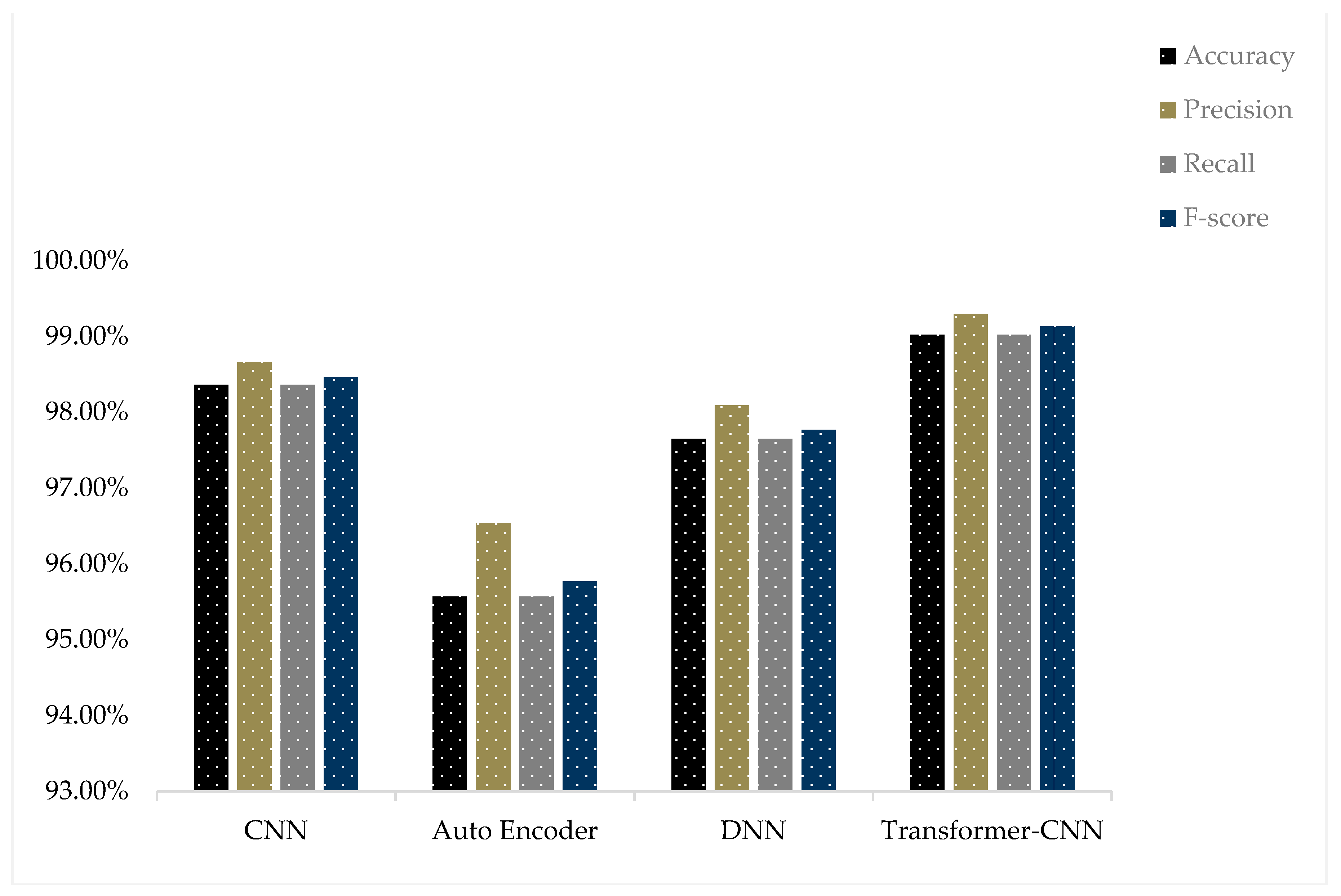
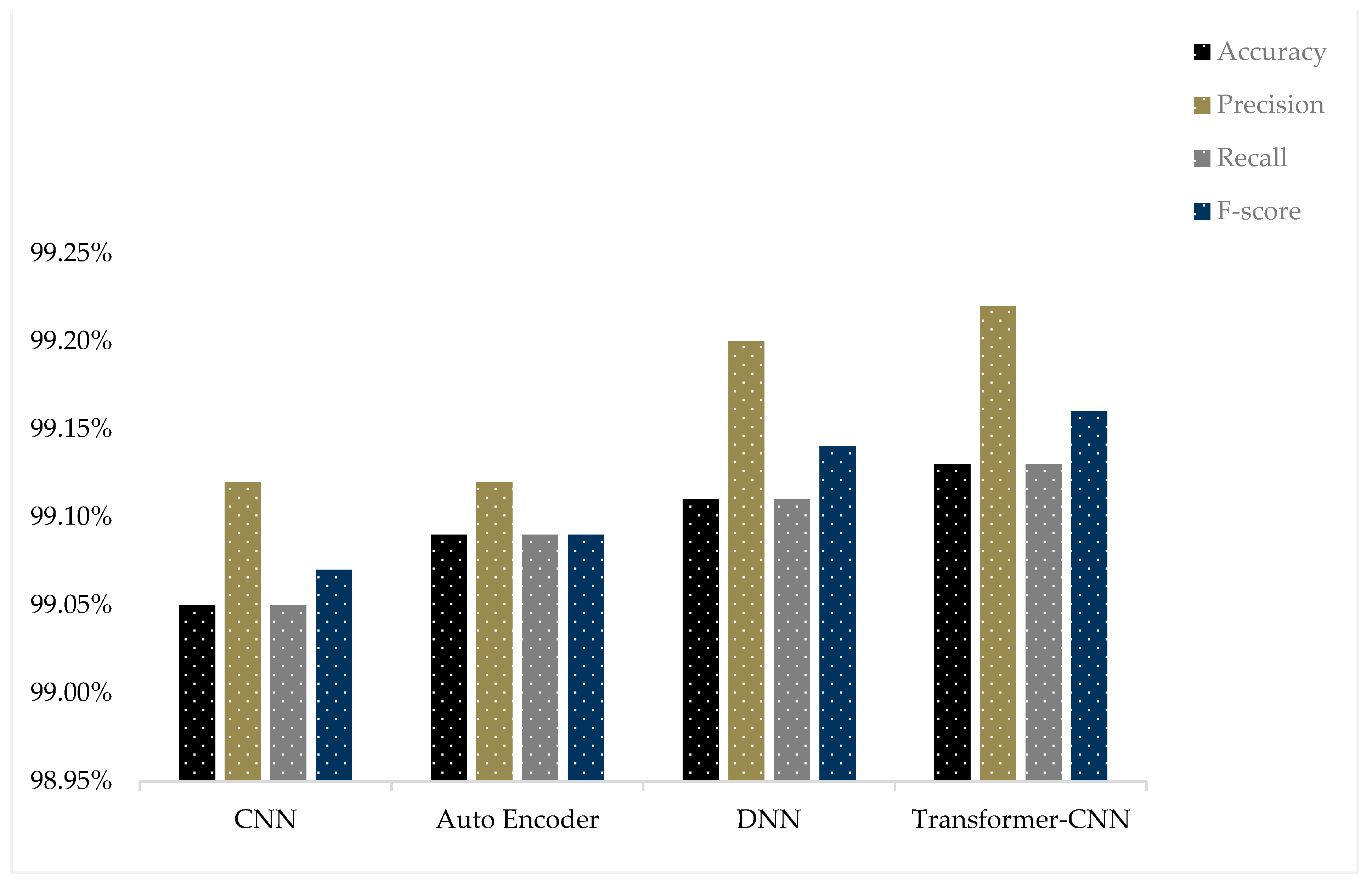
| Dataset | Metric | Accuracy | Precision | Recall | F-Score |
|---|---|---|---|---|---|
| NF-UNSW-NB15-v2 | CNN | 98.36% | 98.66% | 98.36% | 98.46% |
| Auto Encoder | 95.57% | 96.54% | 95.57% | 95.77% | |
| DNN | 97.65% | 98.09% | 97.65% | 97.77% | |
| Transformer-CNN | 99.02% | 99.30% | 99.02% | 99.13% | |
| CICIDS2017 | CNN | 99.05% | 99.12% | 99.05% | 99.07% |
| Auto Encoder | 99.09% | 99.12% | 99.09% | 99.09% | |
| DNN | 99.11% | 99.20% | 99.11% | 99.14% | |
| Transformer-CNN | 99.13% | 99.22% | 99.13% | 99.16% |
| Label | Accuracy | Precision | Recall | F-Score |
|---|---|---|---|---|
| Normal | 99.59% | 100% | 99.59% | 99.79% |
| Attack | 100% | 99.01% | 100% | 99.50% |
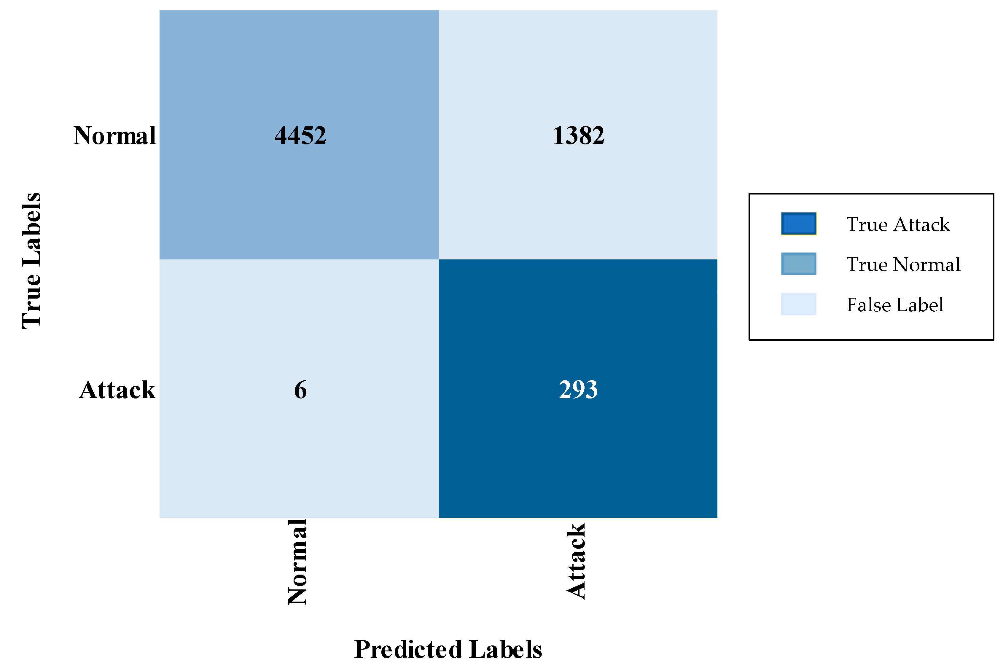
| Label | Accuracy | Precision | Recall | F-Score |
|---|---|---|---|---|
| Normal | 99.89% | 99.98% | 99.89% | 99.94% |
| Attack | 99.97% | 99.86% | 99.97% | 99.92% |
| Label | Accuracy | Precision | Recall | F-Score |
|---|---|---|---|---|
| Benign | 99.63% | 100% | 99.63% | 99.81% |
| Exploits | 96.90% | 99.31% | 96.90% | 98.09% |
| Fuzzers | 99.16% | 97.93% | 99.16% | 98.54% |
| Reconnaissance | 99.42% | 98.29% | 99.42% | 98.85% |
| Generic | 93.62% | 100% | 93.62% | 96.70% |
| DoS | 97.44% | 92.68% | 97.44% | 95% |
| Shellcode | 100% | 100% | 100% | 100% |
| Backdoor | 87.50% | 45.16% | 87.50% | 59.57% |
| Analysis | 80% | 34.78% | 80% | 48.48% |
| Worms | 100% | 83.33% | 100% | 90.91% |
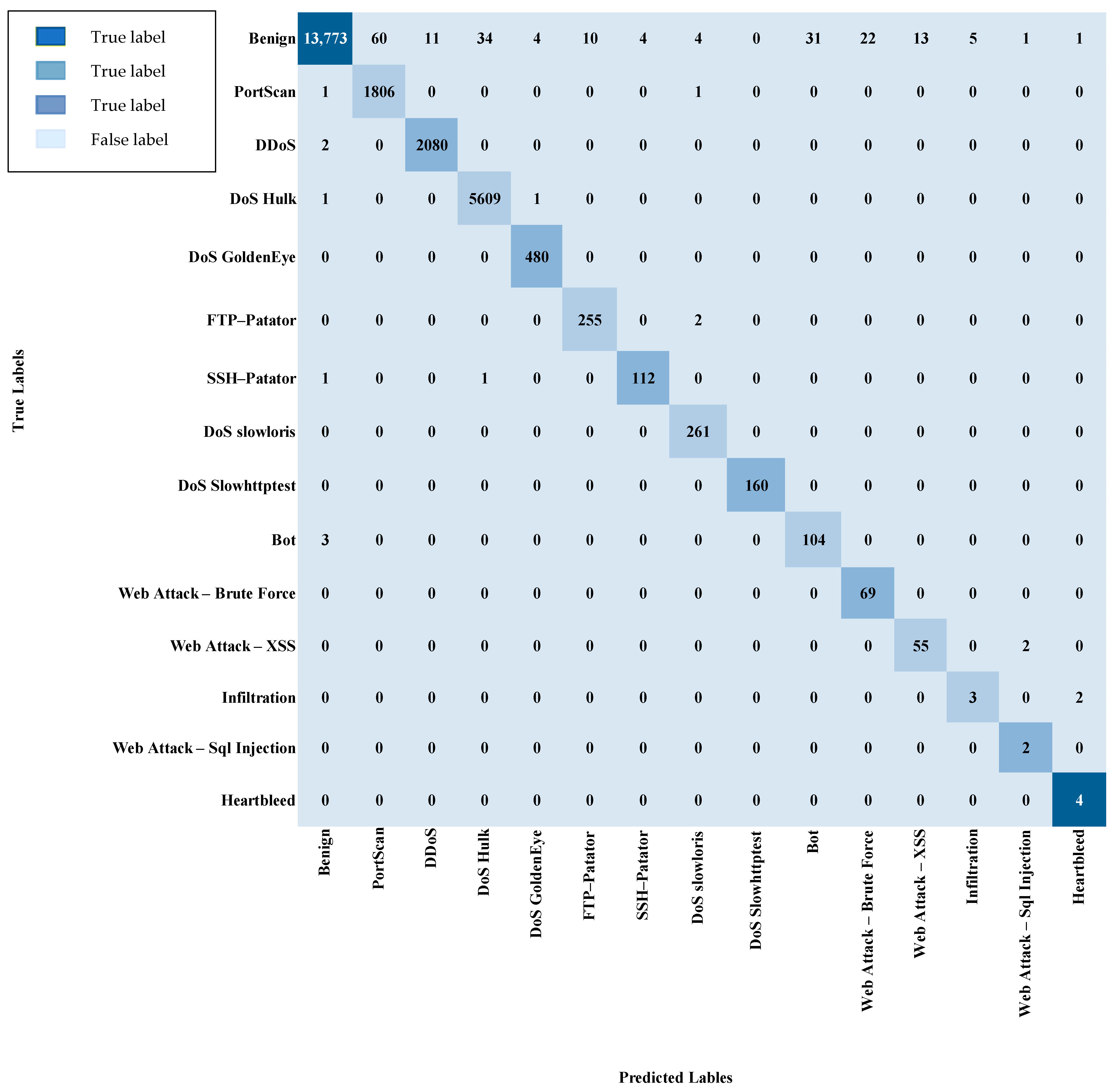
| Label | Accuracy | Precision | Recall | F-Score |
|---|---|---|---|---|
| Benign | 98.57% | 99.94% | 98.57% | 99.25% |
| PortScan | 99.89% | 96.78% | 99.89% | 98.31% |
| DDoS | 99.90% | 99.47% | 99.90% | 99.69% |
| DoS Hulk | 99.96% | 99.38% | 99.96% | 99.67% |
| DoS GoldenEye | 100% | 98.97% | 100% | 99.48% |
| FTP-Patator | 99.22% | 96.23% | 99.22% | 97.70% |
| SSH-Patator | 98.25% | 96.55% | 98.25% | 97.39% |
| DoS slowloris | 100% | 97.39% | 100% | 98.68% |
| DoS Slowhttptest | 100% | 100% | 100% | 100% |
| Bot | 97.20% | 77.04% | 97.20% | 85.95% |
| Web Attack–Brute Force | 100% | 75.82% | 100% | 86.25% |
| Web Attack–XSS | 96.49% | 80.88% | 96.49% | 88% |
| Infiltration | 60% | 37.50% | 60% | 46.15% |
| Web Attack–Sql Injection | 100% | 40% | 100% | 57.14% |
| Heartbleed | 100% | 57.14% | 100% | 72.73% |
Disclaimer/Publisher’s Note: The statements, opinions and data contained in all publications are solely those of the individual author(s) and contributor(s) and not of MDPI and/or the editor(s). MDPI and/or the editor(s) disclaim responsibility for any injury to people or property resulting from any ideas, methods, instructions or products referred to in the content. |
© 2024 by the authors. Licensee MDPI, Basel, Switzerland. This article is an open access article distributed under the terms and conditions of the Creative Commons Attribution (CC BY) license (https://creativecommons.org/licenses/by/4.0/).
Share and Cite
Kamal, H.; Mashaly, M. Advanced Hybrid Transformer-CNN Deep Learning Model for Effective Intrusion Detection Systems with Class Imbalance Mitigation Using Resampling Techniques. Future Internet 2024, 16, 481. https://doi.org/10.3390/fi16120481
Kamal H, Mashaly M. Advanced Hybrid Transformer-CNN Deep Learning Model for Effective Intrusion Detection Systems with Class Imbalance Mitigation Using Resampling Techniques. Future Internet. 2024; 16(12):481. https://doi.org/10.3390/fi16120481
Chicago/Turabian StyleKamal, Hesham, and Maggie Mashaly. 2024. "Advanced Hybrid Transformer-CNN Deep Learning Model for Effective Intrusion Detection Systems with Class Imbalance Mitigation Using Resampling Techniques" Future Internet 16, no. 12: 481. https://doi.org/10.3390/fi16120481
APA StyleKamal, H., & Mashaly, M. (2024). Advanced Hybrid Transformer-CNN Deep Learning Model for Effective Intrusion Detection Systems with Class Imbalance Mitigation Using Resampling Techniques. Future Internet, 16(12), 481. https://doi.org/10.3390/fi16120481