Machine Learning Based Localization of LoRa Mobile Wireless Nodes Using a Novel Sectorization Method

Abstract

Indoor localization of wireless nodes is a relevant task for wireless sensor networks with mobile nodes using mobile robots. Despite the fact that outdoor localization is successfully performed by Global Positioning System (GPS) technology, indoor environments face several challenges due to multipath signal propagation, reflections from walls and objects, along with noise and interference. This results in the need for the development of new localization techniques. In this paper, Long-Range Wide-Area Network (LoRaWAN) technology is employed to address localization problems. A novel approach is proposed, based on the preliminary division of the room into sectors using a Received Signal Strength Indicator (RSSI) fingerprinting technique combined with machine learning (ML). Among various ML methods, the Gated Recurrent Unit (GRU) model reached the most accurate results, achieving localization accuracies of 94.54%, 91.02%, and 85.12% across three scenarios with a division into 256 sectors. Analysis of the cumulative error distribution function revealed the average localization error of 0.384 m, while the mean absolute error reached 0.246 m. These results demonstrate that the proposed sectorization method effectively mitigates the effects of noise and nonlinear signal propagation, ensuring precise localization of mobile nodes indoors.

1. Introduction

In recent years, the accelerated growth of Internet of Things (IoT) devices, along with rapid development in machine learning (ML), has substantially increased the demand for location-based technologies [1]. The advancement of indoor mobile robots, driven by ongoing innovations in sensor technologies and information systems, presents substantial economic opportunities in sectors such as industry, logistics, and transportation [2]. Mobile robots are progressively replacing manual tasks related to cargo handling, monitoring, and hazardous operations, while ensuring continuous automation and unmanned control [3].

In open environment, GPS technology is predominantly used to determine location [4,5]. However, its effectiveness diminishes indoors, as satellite signals are significantly weakened when passing through walls, roofs, and other building structures. This leads to a reduction in accuracy and can even make device localization impossible. An alternative approach is the use of Low Earth Orbit (LEO) satellite systems, which, being closer to Earth, provide location services that support GPS functions [6,7]. With a stronger signal compared to high-orbit satellites, LEO systems are promising for improved coverage and accuracy in dense urban environments. However, their ability to penetrate buildings remains limited, potentially requiring additional solutions for accurate indoor positioning.

Researchers have proposed various types of infrastructure for indoor positioning systems, including wireless sensor networks (WSNs), optical systems, radio frequency technologies, and others. Currently, commonly used indoor positioning technologies encompass visible light communication (VLC), infrared (IR), light detection and ranging (LiDAR), and computer vision [8,9,10]. Although LiDAR and computer vision are effective technologies, they demand high-cost hardware and substantial computing resources. In contrast, IR and VLC systems face limitations due to the short operational range and their dependence on external lighting conditions and transmission angles [11]. These factors reduce their reliability in environments with variable lighting and intricate room geometries [12].

Wireless technologies employed for node localization include Wi-Fi, Ultra-Wideband (UWB), Bluetooth Low Energy (BLE), Radio Frequency Identification (RFID), Zigbee, and LoRaWAN [13,14,15,16,17]. Among the above, LoRaWAN emerges as a promising low-power solution, which is particularly beneficial for mobile devices. In comparison to Wi-Fi, LoRaWAN provides more stable indoor connectivity due to its high signal penetration through obstacles, while global navigation satellite systems (GNSS) and Wi-Fi are not optimal in terms of power consumption for outdoor and indoor applications. Our study investigates the use of LoRa technology for indoor localization using RSSI fingerprinting. Although LoRa technology has been widely studied for outdoor use, research on its indoor application remains limited. In the articles [18,19], the authors identified LoRa as one of the promising new technologies for indoor localization. Islam, Bashima, et al. compared LoRa technology with popular wireless technologies such as BLE and WiFi for indoor localization by analyzing their performance in various indoor line-of-sight and non-line-of-sight scenarios [20]. The authors concluded that LoRa is a viable choice for indoor localization, especially in scenarios requiring low power consumption and wide coverage.

In wireless sensor networks, there are localization methods based on parameters such as angle of arrival (AoA) and time of arrival (ToA) [21,22], which have limitations connected with high equipment cost and insufficient accuracy in the presence of interference and multipath signals. Although [23,24] discuss localization approaches that estimate the phase difference using the AoA identification using I/Q and phase interferometry, there are some nuances in their use indoors. The phase difference and angle measurements are highly dependent on the signal quality, and indoor noise or multipath propagation can distort the results. Indoors, reflections from walls, ceilings, and furniture can cause errors, creating false paths and complicating accurate direction determination. These factors limit the applicability of AoA and interferometry methods in real-world conditions, especially in indoor localization. Consequently, utilizing the received signal strength indicator (RSSI) is often more advantageous. Wireless RSSI technology has proven to be an effective method for range determination, due to its simplicity and practicality. By measuring the signal strength received from a transmitter, RSSI enables the estimation of distance between devices without the need for complex or costly sensors [25].

Recently, ML technologies have advanced significantly to enhance localization accuracy. These approaches facilitate the efficient processing of large volume data while considering various factors that influence the precision of location determination [26]. ML techniques enable the usage of RSSI signals from LoRa devices for fingerprint-based localization. The indoor fingerprint positioning method relies on the establishment of a database that contains pre-measured signal levels from various access points located in designated areas within the premises [27].

Under ideal indoor conditions, the distance can be estimated using RSSI measurements through the following empirical equation:

$$RSSI=-10n\log \left(d\right)+C$$

(1)

where d represents the distance from the deployed sensor node to the base node, n denotes the path loss exponent, and C is a constant [28]. However, in real-world conditions, signals are affected by numerous interferences, including multipath reception caused by reflections and diffraction, interference from other signals within the frequency band, shadowing, and other factors that reduce accuracy. To address this issue, a variety of algorithms have been proposed [29], which effectively filter out noise and aim to minimize the impact of these interfering factors. While RSSI-based localization has certain drawbacks, including potential errors due to environmental factors, advancements in machine learning and statistical modeling techniques are enhancing the accuracy of these systems. As a result, RSSI-based localization represents a significant and promising area of research with the potential to impact a wide range of applications, including asset monitoring, inventory management, healthcare, and emergency response [30,31] to provide wireless communication over long distances with low data rates. In [32], experiments were conducted using trilateration without continuous retraining to demonstrate the capabilities of LoRa for localizing static nodes indoors. In [33], a localization method leveraging LoRa technology is proposed, incorporating Gaussian filtering for data preprocessing to eliminate significant errors.

An analysis of the current literature reveals a notable trend: wireless sensor networks that employ machine learning methods are pivotal in indoor localization technologies. The fingerprint-based localization method, which relies on measuring RSSI, offers a cost-effective and energy-efficient solution. Various approaches to data preprocessing are discussed, including the application of different filters and techniques aimed at reducing noise and enhancing signal accuracy. However, much of the existing research concentrates on static nodes and data collection, neglecting the dynamics of mobile nodes. In traditional fingerprinting methods, RSSI measurements are taken multiple times using a stationary node placed at predetermined grid points, with a fixed distance between the nodes. The accuracy of localizing moving nodes decreases due to variations in their relative positions in space during data transmission. The main contributions of this work are as follows:

(1)

A method for data collection using a mobile LoRa node is proposed, accounting for the dynamics of its movement.

(2)

A method for partitioning the experimental area into sectors is introduced, which minimizes the impact of noise and the nonlinearity of signal propagation in areas with significant deviations within the room.

(3)

Entirely new routes, distinct from the training data, are utilized as a test sample, allowing for an objective evaluation of the models’ performance at previously unknown locations.

The paper is organized as follows: following the introduction, Section 2 presents related works. Section 3 focuses on the methodology, detailing the ML models applied for localization. Section 4 describes the experimental setup, including the environment and tools used for data collection. Section 5 presents the results from the experiments, analyzing the accuracy of the employed methods. Finally, Section 6 concludes the paper by summarizing the key findings and offering suggestions for future research. The paper concludes with a bibliography listing all sources referenced in this study.

2. Related Work

Recent studies have demonstrated the effectiveness of integrating machine learning techniques with LoRa technologies to address indoor localization tasks. In the study [34], various ML methods, such as support vector regression (SVR), spline models, decision trees, and ensemble learning, were applied to solve the RSSI-based localization problem in LoRa networks. However, these models primarily address static localization settings and do not dynamically adapt to real-time environmental changes, reducing their effectiveness for applications involving mobile devices. In [35], a localization algorithm for indoor environments based on LoRa fingerprinting and particle swarm optimization is proposed. The suggested fingerprinting algorithm utilizes multiple wireless signal sources to establish a correlation between RSSI values and coordinates. The initial position is determined using trilateration to enhance accuracy and is further refined with a Bayesian algorithm. While effective for controlled, predefined setups, the method’s reliance on extensive preprocessing can limit adaptability, as expanding the setup would require significant computational resources and processing time to maintain accuracy. The study [36] introduces a filter to eliminate outliers, leveraging log-normal shadowing and a back-propagation neural network (BPNN) to predict unknown locations. Although this approach improves localization accuracy, it relies on the quality of pre-collected data and outlier filtering, and the use of the Log-normal Shadowing Model reduces its effectiveness in complex multi-path environments, limiting its robustness in dynamic conditions.

In [37], the authors developed a low-power intelligent indoor localization system based on RSSI data from LoRaWAN networks, employing random neural networks (RNNs). Purohit et al. proposed a fingerprint-based localization system for indoor and outdoor environments that incorporates interpolation techniques and a denoising autoencoder to eliminate missing and noisy data in LoRa networks [38]. Using deep learning models, such as Artificial Neural Networks (ANN), Long Short-Term Memory (LSTM), and Convolutional Neural Networks (CNN), the system demonstrates superior localization accuracy compared to traditional machine learning methods. In [39], Suroso et al. applied interpolation methods using a random forest algorithm to reduce the time and effort required for fingerprint data collection. They compared the classic pattern matching algorithm with the minimum Euclidean distance algorithm, finding that the random forest algorithm achieved superior results in minimizing maximum estimation errors, while the minimum Euclidean distance algorithm provided higher accuracy. However, these studies are less effective in dynamically changing environments during mobile node movement. The model in [37] relies on predefined anchor placements and requires substantial effort to adapt to shifting configurations, the fingerprint-based system in [38] depends on interpolated data, which necessitates frequent updates to maintain accuracy, and the approach in [39], although effective in reducing data collection time using random forest interpolation, also requires adjustments in dynamic scenarios.

The study [40] introduced a high-precision indoor localization system based on LoRaWAN, measuring both RSSI and SNR from multiple gateways. This method involves transmitting a signal to the gateway, which collects signal data and forwards it to a centralized system for location estimation using ML methods based on neural networks (NNs) to detect or estimate position changes through signal strength variation. While precise, the reliance on SNR as a metric may be limited in direct line-of-sight (LOS) conditions, where SNR often remains stable over short distances and may not effectively capture dynamic changes in mobile node positions. In [41], a deep learning-based indoor localization model was introduced, utilizing LoRa and RSSI fingerprinting. The proposed system, DeepFi-LoRaIn, integrates RSSI fingerprints with deep learning techniques to enhance localization in dynamic environments, accounting for interference and changing environmental conditions. While robust against interference, this model requires frequent retraining to maintain accuracy in varying environments, which can become impractical in deployments where continuous updates are challenging. In [42], the authors presented the Extreme RSS (ERSS) method to stabilize the fingerprint database and formulated boundary autocorrelation to significantly reduce search complexity while improving localization accuracy. Although computationally efficient, this approach requires extensive reference point setup, making it costly and challenging to implement across environments where regular adjustments are needed.

Our approach addresses the limitations identified in these studies, which rely on static data collection methods, fail to account for dynamic environmental changes during data acquisition, and lack validation on unknown test data, making them less adaptable and effective in practical applications.

3. Methodology

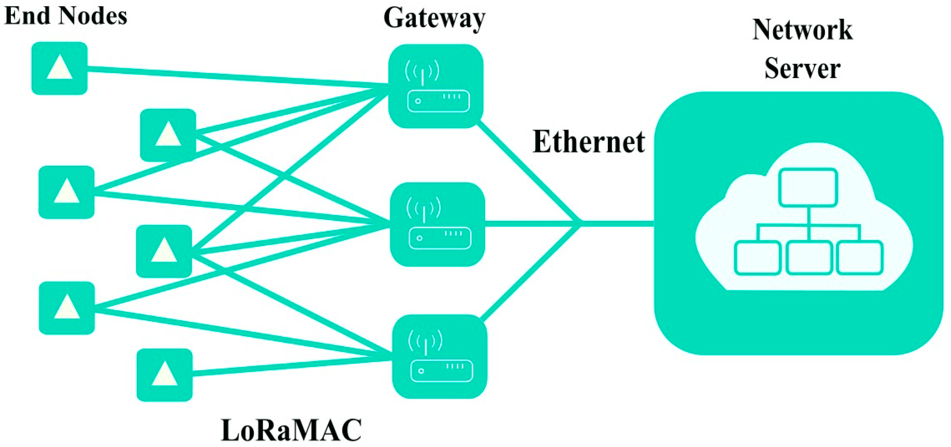
3.1. Overview of LoRaWAN and LoRa Technology

The LoRaWAN Media Access Control (MAC) protocol is an open standard established by the LoRa Alliance, operating above the LoRa physical layer [43]. It outlines the network structure and interactions among three key components of the network:

• end devices or nodes, which operate in a star topology and gather data that are subsequently transmitted to the network;
• gateways, which serve as coordinators among the nodes, receiving data from end devices and forwarding to the network server;
• LoRaWAN network server, responsible for managing and processing the data.

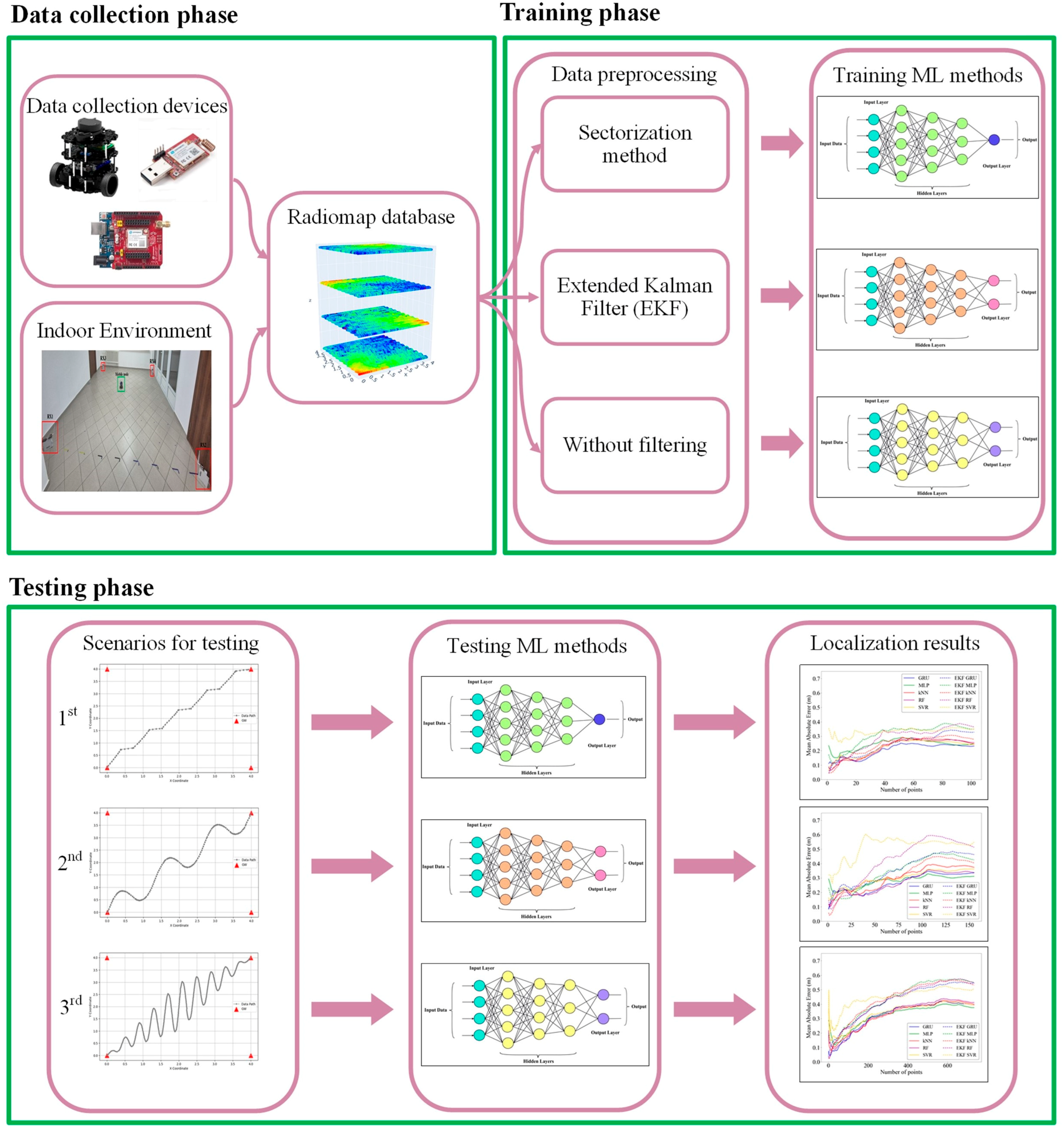
The LoRaWAN network architecture is characterized by a star topology, in which end devices communicate solely with LoRaWAN gateways and do not directly interact with each another. These gateways are connected to a central network server and are in charge for transmitting raw data from end devices to the network server as UDP/IP packets. The network server, connected to the gateways via Ethernet (802.3), manages the transmission of downlink packets and sends control signals to the end devices, which the gateways convert and transmit over the LoRaWAN radio channel. Further communication is established with application servers, which may be operated by third-party organizations, enabling a single network server to support multiple application layers [44]. The LoRaWAN architecture is depicted in Figure 1 below.

LoRa is an affordable wireless modulation technique with a long range capabilities, easily integrable into a network, and utilizing linear spread spectrum technology on unlicensed frequencies [45]. It decreases interference through forward error correction (FEC) and requires minimal infrastructure.

LoRa has been successfully tested indoors, demonstrating stable connectivity even in the presence of multiple obstacles. In [46], the authors evaluated LoRa’s performance, finding that at short ranges, the RSSI is high when the propagation factor is low. However, at greater distances from the gateway, interference increases significantly, necessitating the cooperation of end devices with higher propagation factors. In [47], extensive experiments were conducted with various spreading factor (SF) values. The findings indicate that SF = 7 is optimal for indoor localization using LoRa at short ranges, as it enables more accurate RSSI measurements while providing a higher data rate and lower latency compared to higher SF values like SF = 12, which extend range but compromise positioning accuracy.

Based on previous studies, the following LoRa parameters are optimal for signal transmission in small indoor spaces: a coding rate of CR = ⅘, a spreading factor of SF = 7, a bandwidth of BW = 125 kHz, and a frequency of 868 MHz. These settings ensure high accuracy and efficient data transmission speed for indoor localization.

3.2. Research Map

This section describes the research framework (Figure 2) for indoor localization of mobile nodes, divided into three phases: data collection, training, and testing.

The data collection phase consists of two stages: gathering RSSI data using a TurtleBot3 mobile robot and LA66 LoRaWAN modules within the indoor environment and generating a radio map. The training phase is also divided into two stages: data preprocessing and model training. This study introduces an innovative preprocessing technique for indoor localization based on sector division and evaluates it against existing data preprocessing approaches. Data collection is conducted using four fixed receiver nodes alongside a mobile node mounted on the TurtleBot3 robot. The radio map visualization is presented and described in more detail in Section 5.1. In the next step, for comparison purposes, we perform preprocessing using the Kalman filter and the sectorization method. As a control measure, a separate copy of the data is sent to the training phase without any preprocessing. During the final step of the second phase, ML is applied using algorithms such as k-nearest neighbors (kNN), support vector regression (SVR), random forests (RF), Gated Recurrent Units (GRU), Multilayer Perceptrons (MLP), Back-Propagation Neural Networks (BPNN) and Random Neural Networks (RNN). A detailed description of each algorithm and the selected hyperparameters is provided in Section 3.4. The metrics used to evaluate the performance of the machine learning algorithms are presented in Section 3.5. Finally, in the testing phase, three distinct movement scenarios for the mobile node are proposed. A comprehensive explanation of these testing scenarios is available in Section 4, titled Experimental Setup. The testing dataset is independent from the training dataset and is not included in the generated radio map. It is a separate dataset, which represents three scenarios for the trajectory of a mobile node in a given room, each varying in complexity.

3.3. Data Preprocessing

Data preprocessing is a crucial step that significantly influences the accuracy of ML models utilized for localization. Techniques such as Kalman filtering, which smooths out noise [48], median filtering to eliminate outliers, and data normalization, which standardizes RSSI values to a uniform scale [49], are commonly employed in this context. Additionally, feature selection algorithms are applied to reduce dimensionality and enhance model performance [50]. These approaches help to mitigate the impact of noise in the data, ultimately leading to improved localization accuracy.

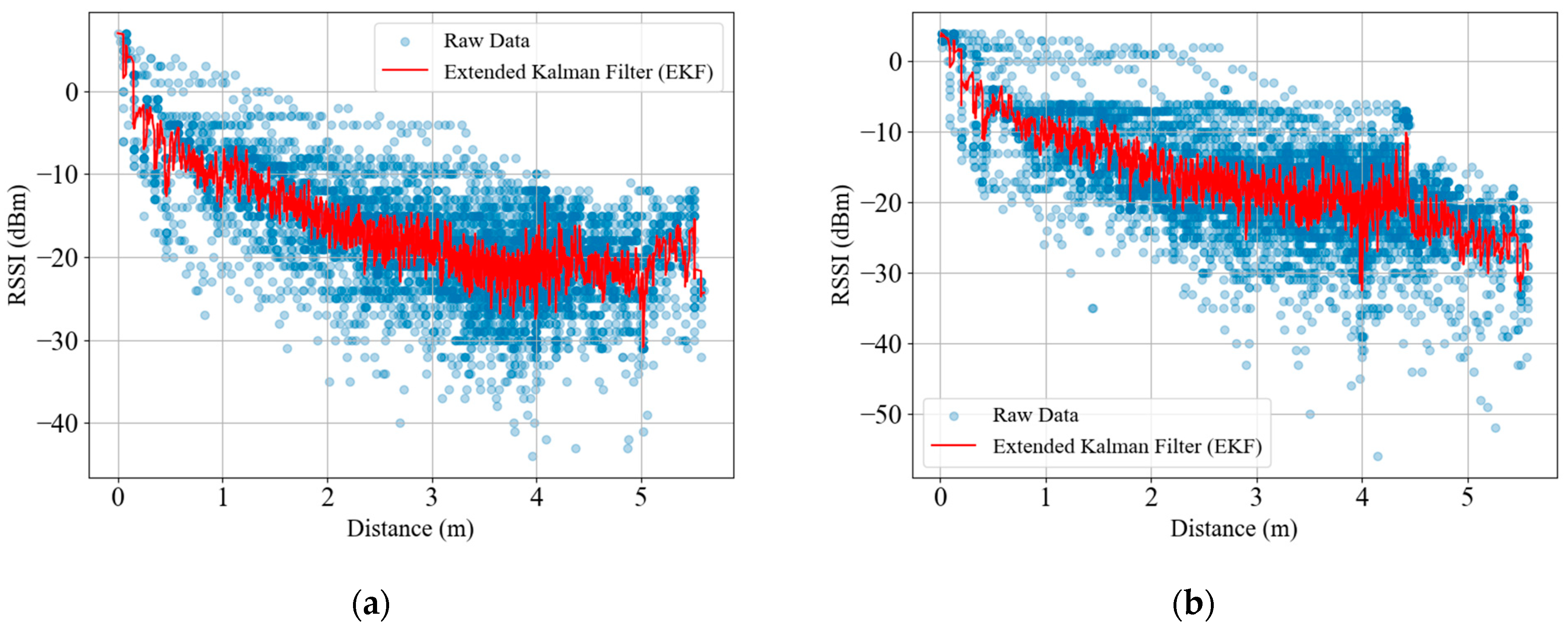
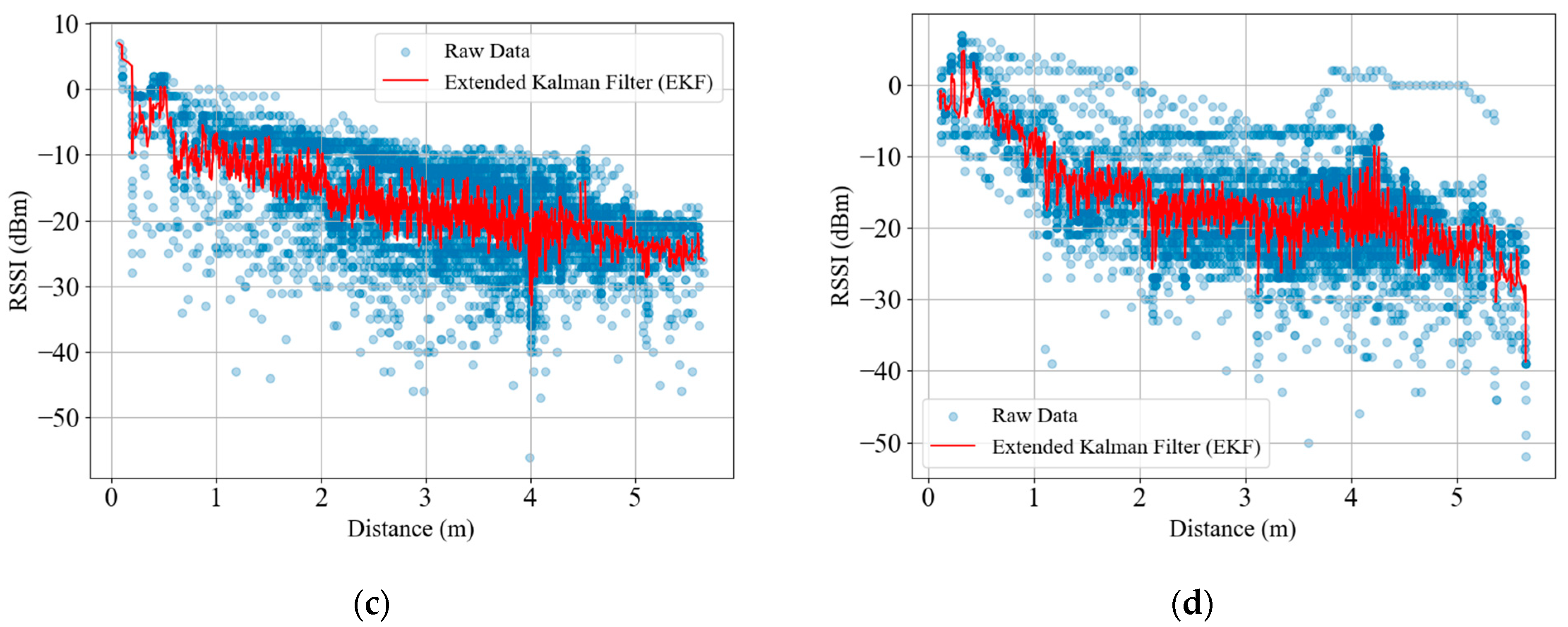
3.3.1. Extended Kalman Filter (EKF)

EKF is an estimation method that optimizes values by minimizing the mean square error. It is particularly effective for estimating parameters of fuzzy models that capture nonlinear relationships. Indoor signal propagation poses several challenges, including reflections from walls, furniture, and other objects, as well as multipath propagation and signal attenuation. All these factors lead to significant nonlinearity in the signal propagation model. EKF effectively addresses these issues by compensating for noise and enhancing the accuracy of the model [51].

The EKF is applied to filter the RSSI data received from four receivers, following these steps.

Firstly, the state and error covariance matrix are predicted:

$${\widehat{x}}_{\left.k\right|k-1}=A_k{\widehat{x}}_{k-1}$$

(2)

$$P_{\left.k\right|k-1}=A_k{P}_{k-1}{A}_k^T+Q_k$$

(3)

where ${\widehat{x}}_{\left.k\right|k-1}$—a priori state assessment, $P_{\left.k\right|k-1}$—a priori error covariance, $A_k$—state transition matrix, and $Q_k$—process noise covariance.

The measurement model defines the relationship between node coordinates and RSSI measurements from receivers:

$$z_k=h\left({\widehat{x}}_{\left.k\right|k-1}\right)+v_k$$

(4)

$$h\left({\widehat{x}}_{\left.k\right|k-1}\right)=\left[\begin{array}{c}\begin{array}{c}{P}_{t1}-10n{\log }_{10}\left(d_1\right)\\ P_{t2}-10n{\log }_{10}\left(d_2\right)\end{array}\\ P_{t3}-10n{\log }_{10}\left(d_3\right)\\ P_{t4}-10n{\log }_{10}\left(d_4\right)\end{array}\right]$$

(5)

where $d_i=\sqrt{{\left(x-x_i\right)}^2+{\left(y-y_i\right)}^2}$, $(x_i,y_i)$—receiver coordinates, $P_{ti}$—transmitter power, n—attenuation factor.

To linearize the measurement function, the Jacobian is used:

$$H_k={\left.{\displaystyle \frac{\partial h}{\partial x}}\right|}_{{\widehat{x}}_{\left.k\right|k-1}}$$

(6)

where

$$H_k=\left[\begin{array}{c}{\displaystyle \frac{\partial h_1}{\partial x}} {\displaystyle \frac{\partial h_1}{\partial y}} \\ {\displaystyle \frac{\partial h_2}{\partial x}} {\displaystyle \frac{\partial h_2}{\partial y}} \\ {\displaystyle \frac{\partial h_3}{\partial x}} {\displaystyle \frac{\partial h_3}{\partial y}} \\ {\displaystyle \frac{\partial h_4}{\partial x}} {\displaystyle \frac{\partial h_4}{\partial y}} \end{array}\right]$$

(7)

$${\displaystyle \frac{\partial h_i}{\partial x}}=-{\displaystyle \frac{10n\left(x-x_i\right)}{\left(\ln \left(10\right)\right)d_i^2}}, {\displaystyle \frac{\partial h_i}{\partial y}}=-{\displaystyle \frac{10n\left(y-y\right)}{\left(\ln \left(10\right)\right)d_i^2}}$$

(8)

The Kalman coefficient is used to adjust the predicted state based on measurements:

$$K_k=P_{\left.k\right|k-1}{H}_k^T{\left(H_k{P}_{\left.k\right|k-1}{H}_k^T+R_k\right) }^{-1}$$

(9)

where $R_k$—measurement noise covariance.

After receiving measurements, the state is updated:

$${\widehat{x}}_k={\widehat{x}}_{\left.k\right|k-1}+K_k(z_k-h\left({\widehat{x}}_{\left.k\right|k-1}\right))$$

(10)

where $z_k-h\left({\widehat{x}}_{\left.k\right|k-1}\right)$—measurement error.

The error covariance matrix is updated using the following method:

$$P_k=(I-K_k{H}_k)P_{\left.k\right|k-1}$$

(11)

where I is the identity matrix.

During the state update, the Kalman gain is employed to determine the extent to which new measurements should be considered for adjusting the predicted state. In scenarios with high noise levels, the Kalman gain reduces the weight of the new data, thereby mitigating its impact on the estimation. This approach allows the filter to effectively minimize the influence of noise.

Updating the error covariance matrix decreases uncertainty in the state after each update step, which enhances confidence in the estimation of the node’s current position. Therefore, the EKF enables precise estimation of the mobile node’s coordinates, even amidst significant noise encountered during signal propagation indoors.

3.3.2. Sectorization Method

In this study, alongside commonly used filtering methods, we introduce a sector division approach. By dividing the area into sectors, we can gather multiple RSSI measurements within each sector simultaneously. Thus, it was possible to minimize the influence of individual strongly deviated points with RSSI, due to which the regression model of ML achieves high accuracy. We propose and compare two configurations: dividing the area into 256 and 1024 sectors, corresponding to sector sizes of 25 cm and 12.5 cm, respectively (Figure 3). This segmentation is strategically selected, as the dimensions of the mobile node are comparable to the sector sizes, especially when dividing into 1024, which allows us to more accurately determine its location in space. In general, the number of sectors and the size of each sector depend on both the dimensions of the space and the size of the mobile node.

3.4. Machine Learning Methods

The pre-processed and collected data serve as the foundation for training ML prediction models aimed at indoor localization. In addition to widely utilized models, such as k-nearest neighbors (kNN), support vector regression (SVR), and random forests (RFs), we also use advanced algorithms, including Gated Recurrent Units (GRU), Multilayer Perceptrons (MLP), Back-Propagation Neural Networks (BPNN) and Random Neural Networks (RNN).

The hyperparameters for each ML model are optimized using Bayesian optimization in order to enhance accuracy and mitigate the risk of overfitting. The selected parameters for the machine learning models are detailed in each subsection of Section 3.4, in accordance with the names of the algorithms. Grid Search is a hyperparameter optimization technique that involves systematically exploring all possible combinations of hyperparameter values within a predefined range. This approach enables the identification of the most optimal parameters to maximize accuracy or other indicators of model quality.

3.4.1. Support Vector Regression (SVR)

Support Vector Regression (SVR) is an extension of Support Vector Machines (SVM) designed to address regression tasks. SVM is a powerful ML tool used for both classification and regression tasks [52]. It operates based on the principle of maximizing the separating hyperplane between different classes in a multidimensional space. The formulation of this hyperplane is achieved through the following process:

$$minimize{\displaystyle \frac{1}{2}}{‖w‖}^2+C{\sum }_{i=1}^n{\xi }_i$$

(12)

$$subject to y_i\left(w·x_i+b\right)\ge 1-{\xi }_i, \forall x_i {\xi }_i\ge 0$$

(13)

where w is the field width vector, C is the relation between field width and misclassifications, ${\xi }_i$ is a weak variable, a $y_i$ is an equivalent label of $x_i$.

The SVR method is employed to determine the location of mobile nodes in indoor environments based on RSSI fingerprints. SVR analyzes the relationships between trained grid points and their corresponding fingerprints, modeling each point and performing regression to accurately estimate the nodes’ locations. Listed below are the hyperparameters employed for Grid Search optimization:

• Number of neighbors (n_neighbors): {1, 3, 5, 7, 9, 11};
• Weighting scheme (weights): {‘uniform’, ‘distance’};
• Search algorithm (algorithm): {‘auto’, ‘ball_tree’, ‘kd_tree’, ‘brute’};
• Distance metric (p): {1, 2} (1 for Manhattan distance, 2 for Euclidean distance).

3.4.2. k-Nearest Neighbors

k-Nearest Neighbors (kNN) is one of the simplest and most intuitive ML algorithms used for classification and regression problems. It is based on the concept that objects with similar characteristics are located close to each other in a high-dimensional feature space [53].

kNN calculates the distances between the new feature’s dimensions and all points in the training dataset using a selected metric, such as Euclidean or Manhattan distance. The parameter ‘K’ represents the number of nearest neighbors considered. In regression tasks, kNN estimates an unknown value based on the known values of nearby points. The predicted value, $\widehat{y}$, is determined by averaging the target variables of the nearest neighbors [54]:

$$\widehat{y}={\displaystyle \frac{1}{K}}{\sum }_{i=1}^K{y}_i$$

(14)

where yi is the value of the target variable of the i-th neighbor. Listed below are the hyperparameters employed for Grid Search optimization:

• Regularization parameter (C): {0.1, 1, 10, 100};
• Epsilon (epsilon): {0.01, 0.1, 0.2, 0.5};
• Kernel type (kernel): {‘linear’, ‘poly’, ‘rbf’, ‘sigmoid’};
• Kernel parameter (gamma): {‘scale’, ‘auto’}.

3.4.3. Random Forest

Random Forest (RF) is an ensemble learning technique utilized for classification and regression tasks, enhancing prediction accuracy by combining multiple decision trees [55]. Each tree is trained on random subsets of both data and features, which mitigates the risk of overfitting. The bootstrapping method generates numerous unique samples, adding diversity to the model. Due to its resilience to noise, Random Forest performs effectively with large datasets. Additionally, it can assess the importance of features, aiding in the identification of the most significant variables for analysis. The following regression equation is used for localization:

$$\widehat{P}={\displaystyle \frac{1}{n}}{\sum }_{i=1}^n{T}_i\left(X\right)$$

(15)

where: $T_i\left(X\right)$ is prediction of the i-th tree for input data X, n is the total number of trees in a forest. Listed below are the hyperparameters employed for Grid Search optimization:

• Number of trees (n_estimators): {10, 50, 100, 200};
• Maximum tree depth (max_depth): {None, 10, 20, 30, 40, 50};
• Minimum number of samples required to split a node (min_samples_split): {2, 5, 10};
• Minimum number of samples required in a leaf (min_samples_leaf): {1, 2, 4};
• Bootstrap sampling (bootstrap): {True, False}.

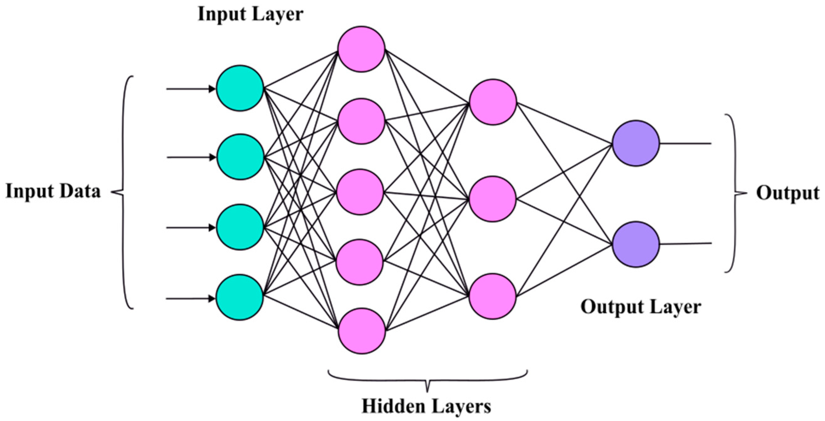
3.4.4. Multilayer Perceptron

A multilayer perceptron (MLP) is a type of artificial neural network consisting of multiple layers of neurons [56]. It serves as a key component in more complex neural network architectures and is widely employed in various ML applications, including classification, regression, and signal processing.

An MLP comprises several layers of neurons as depicted in Figure 4, including an input layer, an output layer, and at least one hidden layer. A multilayer perceptron (MLP) is a fully connected neural network, meaning that each neuron in one layer is linked to every neuron in the subsequent layer. The input layer receives data, which can include numerical or encoded categorical features. Hidden layers are responsible for learning complex relationships within the data; the more hidden layers and neurons present, the more sophisticated the models that can be trained. The output layer generates predictions for specific tasks, whether for regression or classification. Hidden layers commonly employ activation functions, such as ReLU (Rectified Linear Unit), sigmoid, or tanh, enabling the network to capture nonlinear relationships. MLPs are trained using backpropagation, in which the gradients of the loss (error) over the parameters (weights) of the network are calculated and adjusted using an optimization algorithm, such as gradient descent. Listed below are the hyperparameters employed for Grid Search optimization:

• Number of neurons (units): {16, 32, 64, 128};
• Activation function (activation): {‘tanh’, ‘relu’};
• Dropout rate (dropout): {0.0, 0.2, 0.5};
• Recurrent layer dropout rate (recurrent_dropout): {0.0, 0.2, 0.5};
• Optimizer (optimizer): {‘adam’, ‘sgd’};
• Learning rate (learning_rate): {0.001, 0.01, 0.1}.

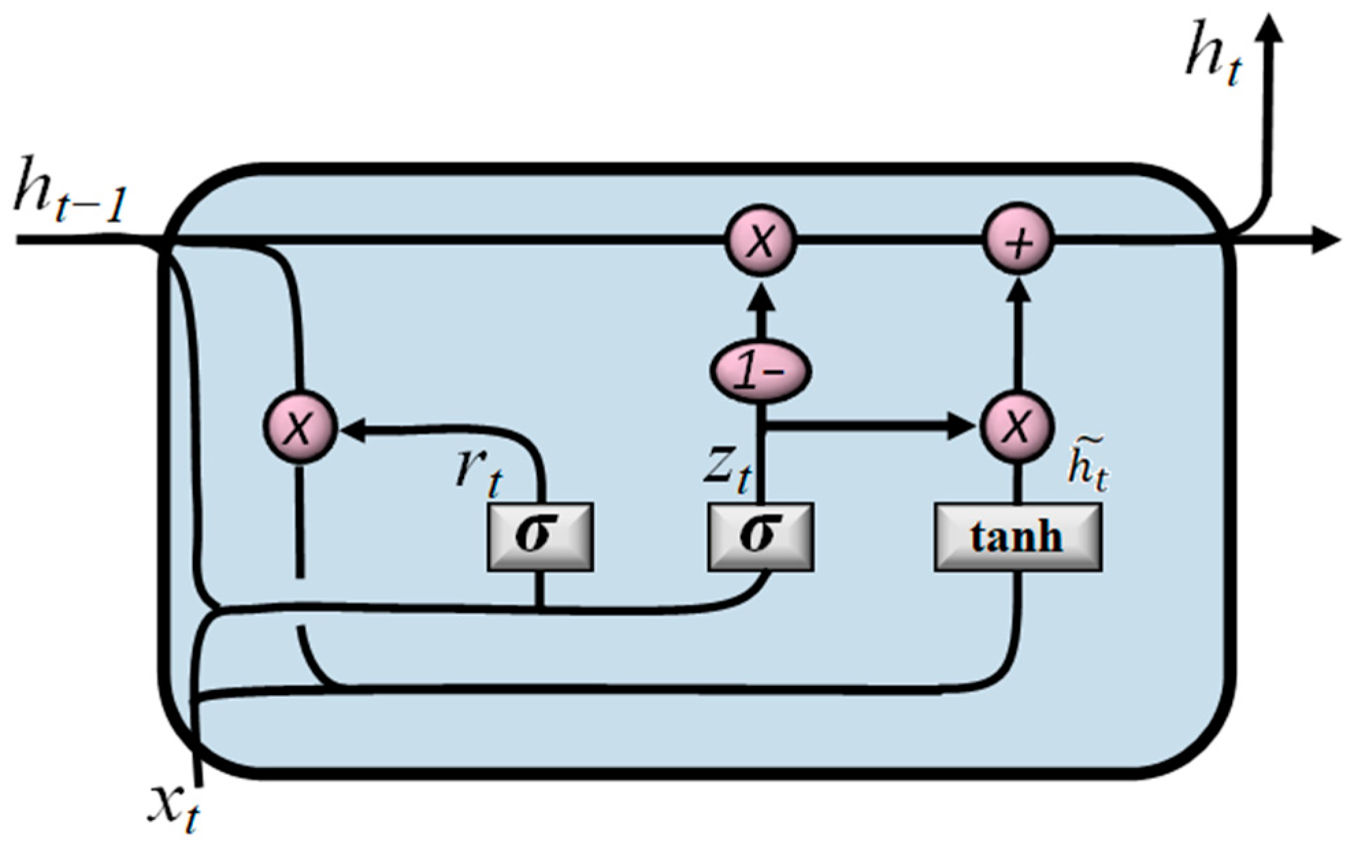
3.4.5. Gated Recurrent Unit

The Gated Recurrent Unit (GRU) is a type of recurrent neural network introduced by Cho et al. in 2014 [57]. GRUs effectively tackle the vanishing gradient problem while ensuring high performance with lower computational costs, making them ideal for real-time applications.

$$z_t=\sigma \left(W_z·\left[h_{t-1},x_t\right]\right)$$

(16)

$$r_t=\sigma \left(W_r·\left[h_{t-1},x_t\right]\right)$$

(17)

$${\tilde{h}}_t=tanh\left(W·\left[{r_t·h}_{t-1},x_t\right]\right)$$

(18)

$$h_t=\left(1-z_t\right)·h_{t-1}+z_t·{\tilde{h}}_t$$

(19)

The Gated Recurrent Unit (GRU) features two control mechanisms: the reset element and the update element, which are neural networks that control the flow of information between time steps (Figure 5). The update module allows the model to determine how much past information to retain or discard, thereby effectively reducing the risk of the vanishing gradient problem. Meanwhile, the reset element allows the model to selectively determine the extent to which past information should be remembered or forgotten. Listed below are the hyperparameters employed for Grid Search optimization:

• Hidden layer size (hidden_layer_sizes): {(50,), (100,), (50, 50), (100, 100)};
• Activation function (activation): {‘identity’, ‘logistic’, ‘tanh’, ‘relu’};
• Optimization method (solver): {‘lbfgs’, ‘sgd’, ‘adam’};
• Regularization parameter (alpha): {0.0001, 0.001, 0.01, 0.1};
• Learning rate change schedule (learning_rate): {‘constant’, ‘invscaling’, ‘adaptive’}.

3.4.6. BPNN

Backpropagation Neural Network (BPNN) is a type of artificial neural network that uses the backpropagation algorithm for training [58]. It consists of layers of neurons: an input layer, one or more hidden layers, and an output layer. Each neuron is connected to neurons in neighboring layers via weights that are updated during the training process.

The BPNN training algorithm involves two stages: forward propagation and backpropagation. In the forward stage, input data is passed through the network, transformed by nonlinear activation functions, and the network generates predictions. In the backpropagation stage, the error is calculated (e.g., using a loss function), which is then propagated back through the network to adjust the weights using gradient descent. This process is repeated until the network minimizes the error. Listed below are the hyperparameters employed for Grid Search optimization:

• Number of neurons (units): {16, 32, 64, 128};
• Number of Hidden Layers (hidden_neurons): {1,2,3}
• Activation function (activation): {‘tanh’, ‘relu’, ‘sigmoid’};
• Dropout rate (dropout): {0.1, 0.2, 0.5};
• Optimizer (optimizer): {‘adam’, ‘sgd’};
• Learning rate (learning_rate): {0.001, 0.01, 0.1}.
• Number of epochs (epochs): {10, 50, 100, 200};
• Momentum: {0.8, 0.9, 0.99}

3.4.7. RNN

Random Neural Network (RNN) is a neural network model proposed by Erol Gelenbe in 1989 [59]. Unlike classical neural networks based on deterministic functions, RNN operates on the basis of probabilistic processes, where neurons are modeled as elements that randomly change their state. Each neuron has two states: active (signal generation) and passive, and transitions between them are determined by probabilities depending on input signals. The peculiarity of the model is that neurons transmit “spikes” to each other—signals that can either excite or suppress other neurons. Network training consists of adjusting probabilistic parameters to achieve the desired result. Listed below are the hyperparameters employed for Grid Search optimization:

• Number of neurons in the hidden layer: [10, 50, 100, 200]
• Number of hidden layers: [1, 2, 3]
• Excitation rate (λ_in): [0.01, 0.1, 1, 10]
• Inhibition rate (λ_out): [0.01, 0.1, 1, 10]
• Connection weights: [−1, −0.5, 0, 0.5, 1])
• Learning rate: [0.001, 0.01, 0.1, 0.5]
• Batch size: [16, 32, 64, 128]
• Activation function: [‘sigmoid’, ‘tanh’, ‘relu’, ‘linear’]
• Dropout rate: [0.0, 0.2, 0.5]
• Number of epochs: [10, 50, 100, 200]

3.5. Performance Metrics

The study employed four established evaluation metrics for regression machine learning tasks to assess the performance of the models.

Mean Absolute Error (MAE): This metric is frequently used in regression tasks to gauge model accuracy. It computes the average of absolute differences between predicted and actual values, providing insight into the average deviation of the model’s predictions from the real data (Equation (20)).

$$MAE={\displaystyle \frac{1}{n}}{\sum }_{i=0}^{n-1}\left(\left|y_i-{\widehat{y}}_i\right|\right)$$

(20)

where $y_i$ is true value, ${\widehat{y}}_i$ is predicted value, and n is the total number of observations.

Root Mean Square Error (RMSE) is a key metric for assessing the accuracy of regression models, reflecting the discrepancy between predicted values and actual observations. RMSE is calculated as the square root of the average of the squared errors, thereby emphasizing larger deviations (Equation (21)).

$$RMSE=\sqrt{{\displaystyle \frac{1}{n}}{\sum }_{i=0}^{n-1}{(y_i-{\widehat{y}}_i)}^2}$$

(21)

where $y_i$ is true value, ${\widehat{y}}_i$ is predicted value, and n is the total number of observations.

R-squared (R²) is a metric that indicates how effectively a model accounts for the variability of the dependent variable, with values ranging from 0 to 1. An R² value close to 1 suggests a good fit between the predicted and actual values, while lower values may indicate poor model quality (Equation (22)).

$$R^2=1-{\displaystyle \frac{{SS}_{res}}{{SS}_{tot}}}$$

(22)

${SS}_{res}$ represents the sum of squared residuals, which measures the differences between actual and predicted values, while ${SS}_{tot}$ denotes the total sum of squares, reflecting the differences between actual values and their mean.

Average Localization Error (AE) is a metric that quantifies the average discrepancy between predicted values and actual values within a dataset. This metric offers valuable insight into the accuracy of a predictive model or algorithm. The AE is presented below:

$$AE={\sum }_{i=1}^n{({\left(X_{real}-X_{pred}\right)}^2+{(Y_{real}-Y_{pred})}^2)}^{0.5}$$

(23)

where $X_{real}$ and $Y_{real}$ are actual coordinates, $X_{pred}$ and $Y_{pred}$ are predicted coordinates, and n is the total number of data points.

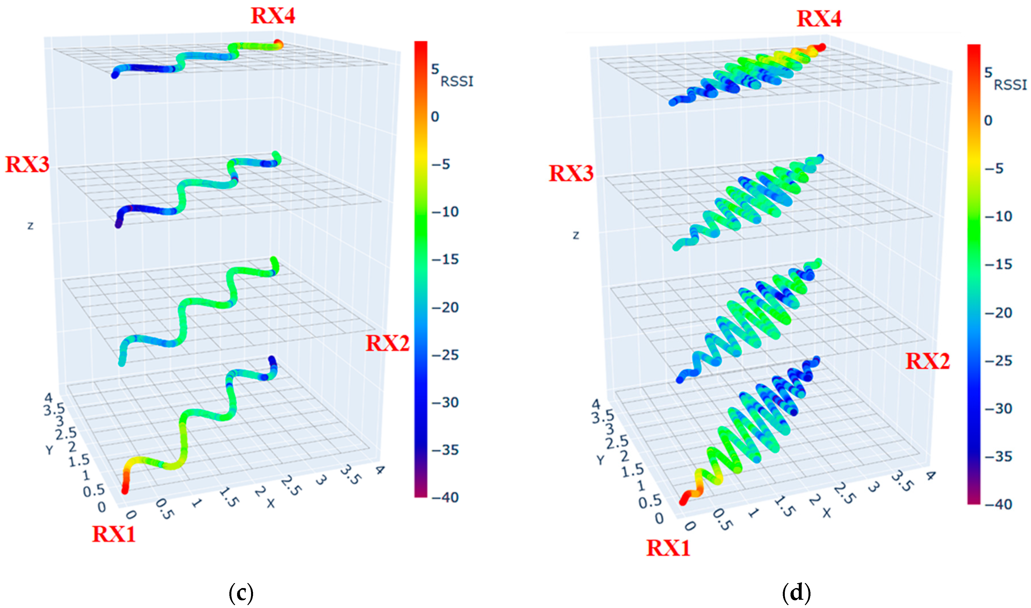
4. Experimental Setup

This section provides a detailed description of the experimental setup. We created an experimental area, illustrated in Figure 6 below, measuring 4 m × 4 m, for collecting RSSI data. In the study [35], two configurations were used with different numbers of gateways (3 and 4) in practical experiments to evaluate different gateway placement strategies. The results showed that increasing the number of gateways improves the localization accuracy. Based on these results, we positioned four receivers at the corners of the experimental area. The reference point for the experimental area is set at coordinates (0,0), where the first receiver is located. All subsequent test routes originate from this reference point.

For data collection, the TurtleBot3 Burger mobile robot (depicted as a green square in Figure 6), the LA66 LoRaWAN Shield (shown as a red square), and a LoRaWAN USB Adapter were utilized. Figure 7A illustrates the TurtleBot3 Burger, developed by Robotis [60]. This compact and lightweight robot is designed for educational and research purposes in robotics and is fully compatible with the Robot Operating System (ROS). The robot is equipped with a 360° LiDAR sensor, which is essential for mapping, localization (SLAM), and navigation. Its modular design allows for easy configuration changes based on specific tasks. The system is powered by a Raspberry Pi 4 single-board computer, which handles data processing and control, operating with the ROS Noetic version for seamless integration and management. Its dimensions are compact, with a length of 138 mm, width of 178 mm, and height of 192 mm. Additionally, the robot features an OpenCR controller based on a 32-bit ARM Cortex M7, providing high performance for managing robotic systems.

The LA66 LoRaWAN Shield and the LoRaWAN USB Adapter were employed for collecting Received Signal Strength Indicator (RSSI) data using a fingerprinting method [61]. In our study, omnidirectional antennas were used at both the receiver and transmitter. The LA66 LoRaWAN served as the receiver, capturing data from devices utilizing the LoRaWAN protocol, while the LoRaWAN USB Adapter acted as the transmitter, connecting to the Raspberry Pi 4 of the TurtleBot3 mobile robot. The LA66 LoRaWAN (Figure 7B) operates in the frequency bands of 433 MHz, 868 MHz, and 915 MHz, achieving a maximum communication range of up to 15 km in open terrain, contingent upon environmental conditions. It is equipped with UART, SPI, and I2C interfaces, facilitating connections with various sensors and devices, making it a versatile solution for numerous applications. The compact design of the LA66 enhances its integration into diverse systems. Meanwhile, the LoRaWAN USB Adapter (Figure 7C) connects to computers and laptops via USB 2.0, ensuring compatibility with most devices. It supports LoRaWAN protocols version 1.0 and above, rendering it adaptable for use with various LoRaWAN devices and platforms. Additionally, both modules exhibit low power consumption, making them suitable for autonomous applications. The parameters of the LA66 LoRaWAN module used in this experiment are presented in detail in

Table 1. The parameters of the LA66 LoRaWAN module.

Parameter	Value
Frequency	868 MHz
Spreading factor (SF)	7
Transmission power (TP)	10 dBm
Bandwidth (BW)	125 kHz
Coding rate (CR)	4/5
Sensitivity	−130 dBm

.

The radio map of the experimental area was generated using a TurtleBot3 robot moving at a low speed while transmitting signals at a frequency of 2 Hz. The movement trajectory for collecting training data is shown in Figure 8. The coordinates during the robot’s movement were obtained using a wheel odometer, starting from the initial point (0,0) and ending at (4,4). The robot moves at a constant speed, with a step of 5 cm for each row. Four radio maps, one from each receiver, will serve as the foundation for building and training models capable of accurately identifying and predicting the object’s location based on the received signals. The input data for these models will consist of RSSI values collected during three different movement scenarios in the testing phase. Figure 8 illustrates the sidewinding trajectory of the robot through the experimental area. Each point on the map corresponds to four RSSI readings from each receiver, along with the horizontal and vertical coordinates, X and Y, respectively.

To test the trained ML models, we propose three distinct scenarios, each featuring a different movement trajectory for the TurtleBot3 Burger mobile robot. The robot’s movement paths in these test scenarios are illustrated in Figure 9. Similar to the process of creating the radio map for training data, the robot transmitted signals at a frequency of 2 Hz. Its speed varied between 2 cm/s and 22 cm/s, depending on the chosen route. The three selected paths are illustrated in Figure 9 below:

(a)

The first scenario—movements along a step trajectory;

(b)

The second scenario—movements along a sinusoidal trajectory;

(c)

The third scenario—movements along a sinusoidal trajectory with high amplitude and frequency.

The first route involves a stepped diagonal movement across the experimental area. This trajectory can be considered easy, as it contains fewer turns, and most of the path is straight, which allows the robot to move at maximum speed. The second route follows a sinusoidal trajectory, which presents more complexity than the first due to its smooth curves, necessitating that the robot reduce its speed. In the final route, both the amplitude and frequency of the sinusoidal trajectory from the second route are increased, making it the most challenging. During the more difficult turns, the robot moved at a minimum speed of 2 cm/s.

5. Results

This section presents the results of experiments and data preprocessing, including an evaluation of ML models. The first part focuses on the radio map of the area, the second on data preprocessing, and the third on assessing the accuracy of the ML models.

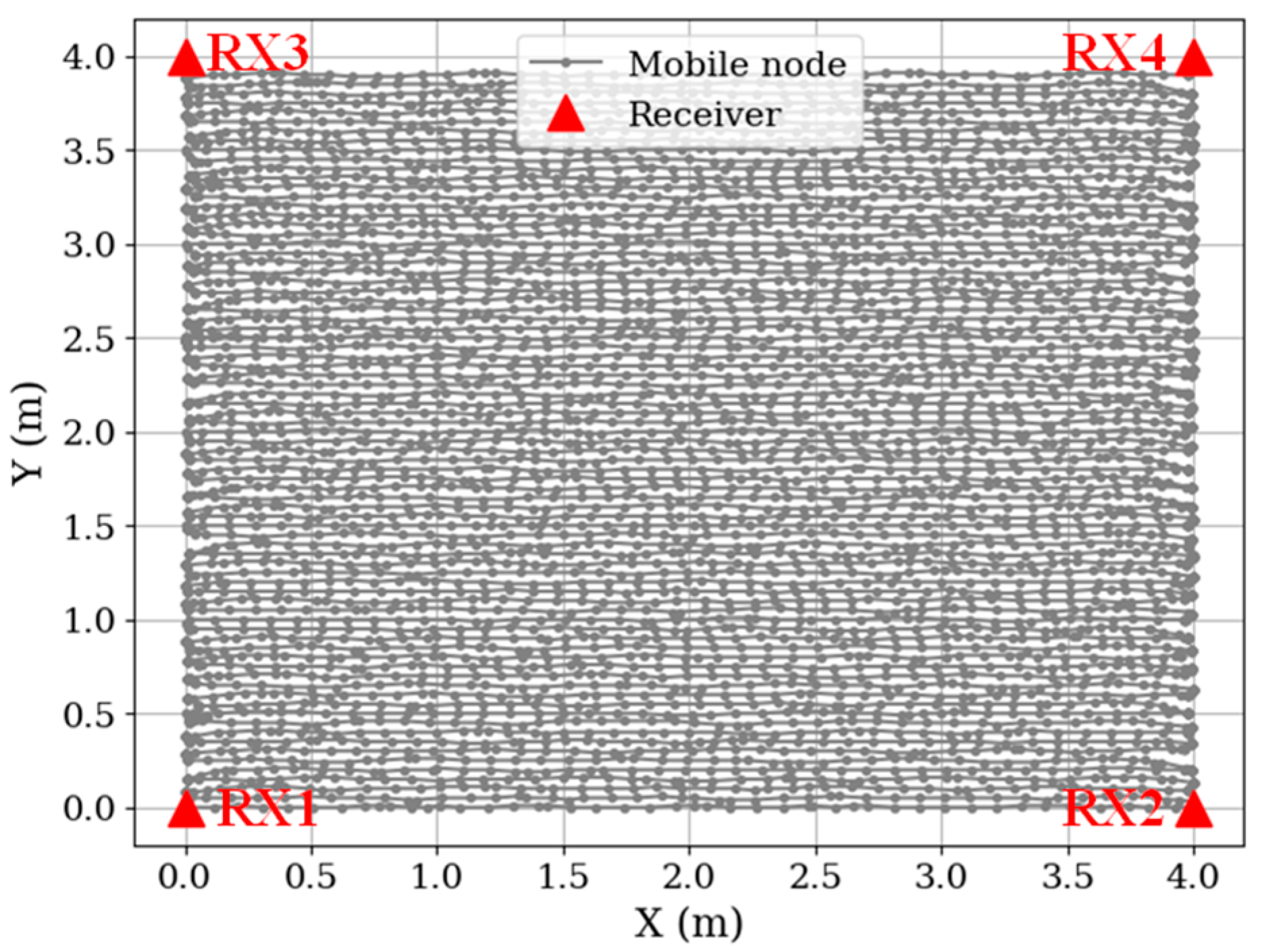
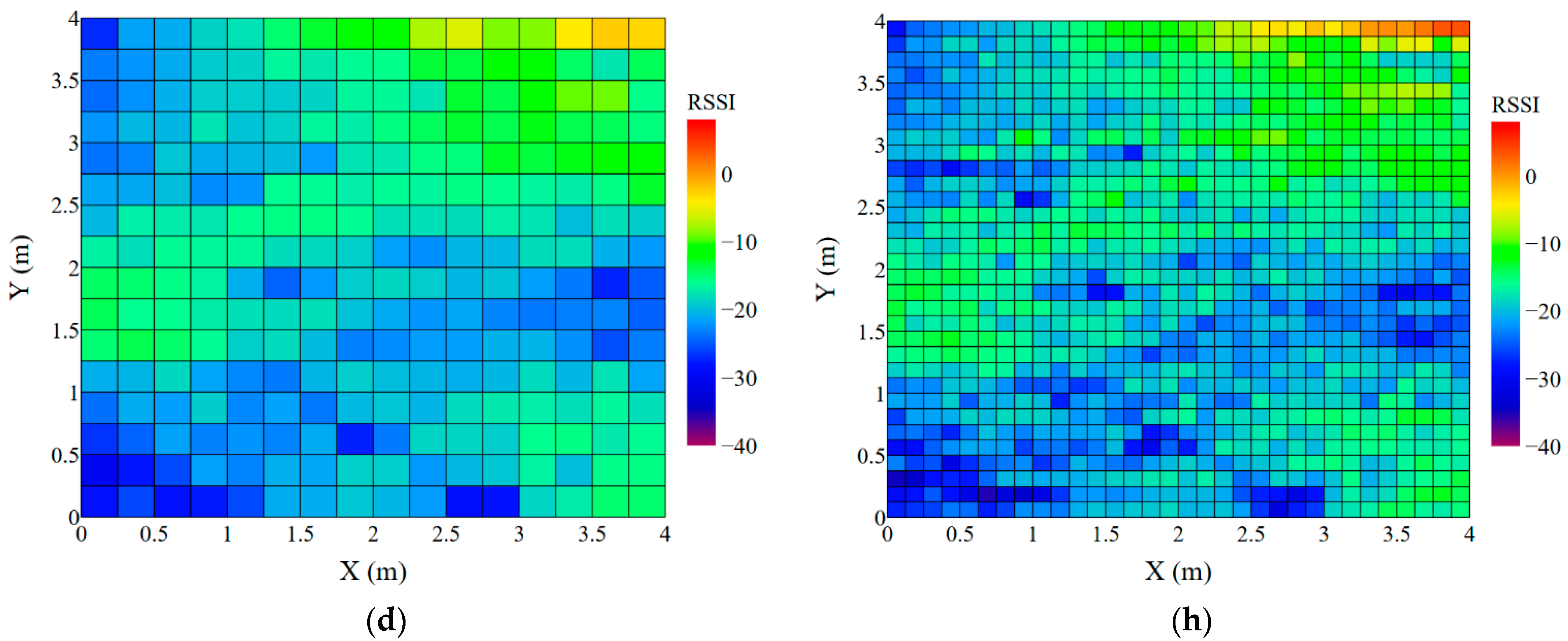
5.1. Radio Map of the Area

Figure 10 illustrates the generated radio map of the experimental area and the test movement routes. Each layer of the map corresponds to the received RSSI signals from each receiver. With four receivers utilized, the radio map comprises four distinct layers. Each point is associated with coordinates obtained from the odometer, and the color of the point reflects the RSSI value: red indicates higher values, while blue indicates lower ones. As observed from the radio map, the signal strength decreases as the distance from the corresponding receiver increases.

However, it is important to note that some points deviate significantly from the general trend of RSSI variation. This deviation may be caused by signal reflections from walls and interference.

5.2. Data Preprocessing Results

This section provides the results of data preprocessing for the methods described in Section 3.4. Figure 11 illustrates how EKF operates for each receiver. The x-axis represents the distance of our node from the corresponding receiver, while the y-axis displays the RSSI values.

A common radio map was built using the filtered RSSI data from each receiver. As illustrated in Figure 12 below, the RSSI coverage exhibits smoother transitions.

Figure 13 presents the results of dividing the area into 256 and 1024 sectors. The left column shows the results for the 256-sector division, while the right column displays the results for the 1024-sector division for each receiver.

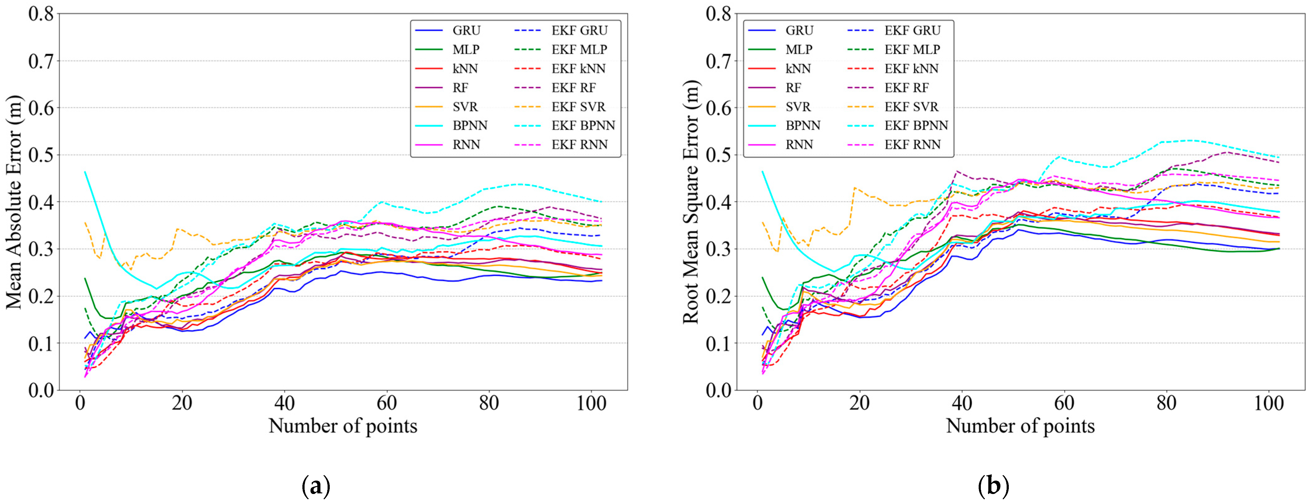
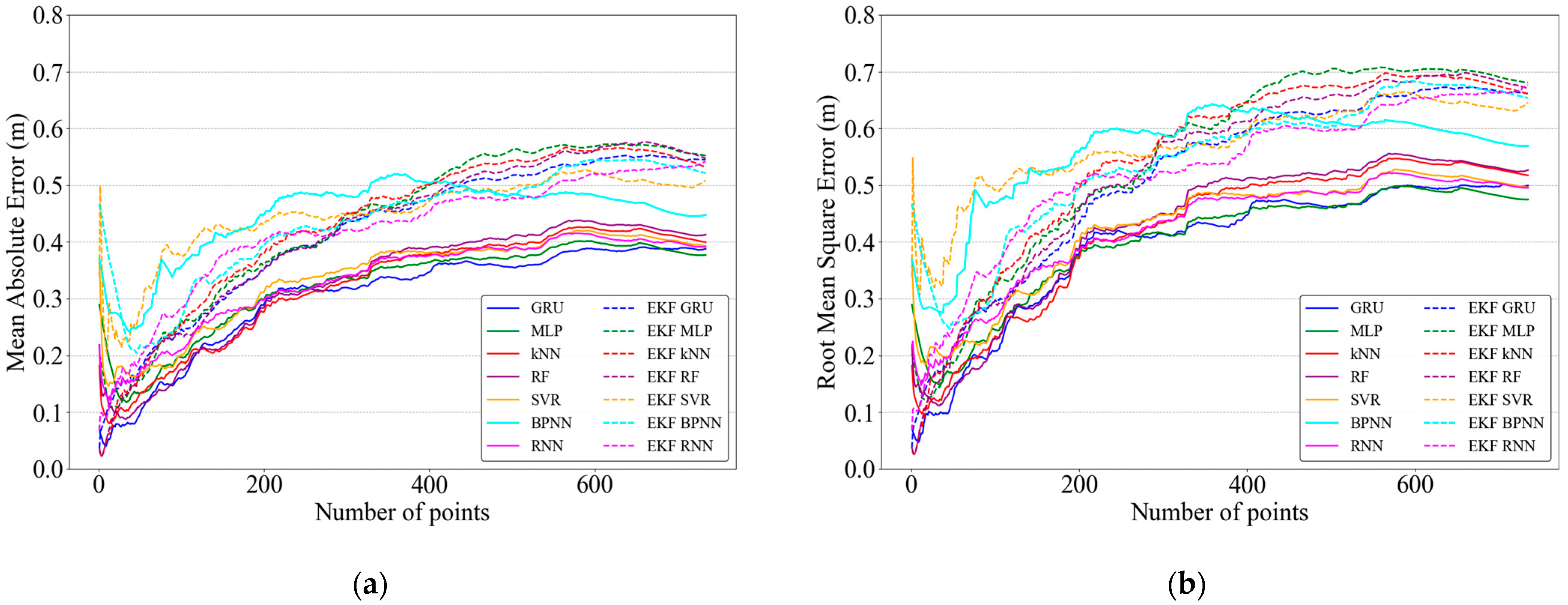
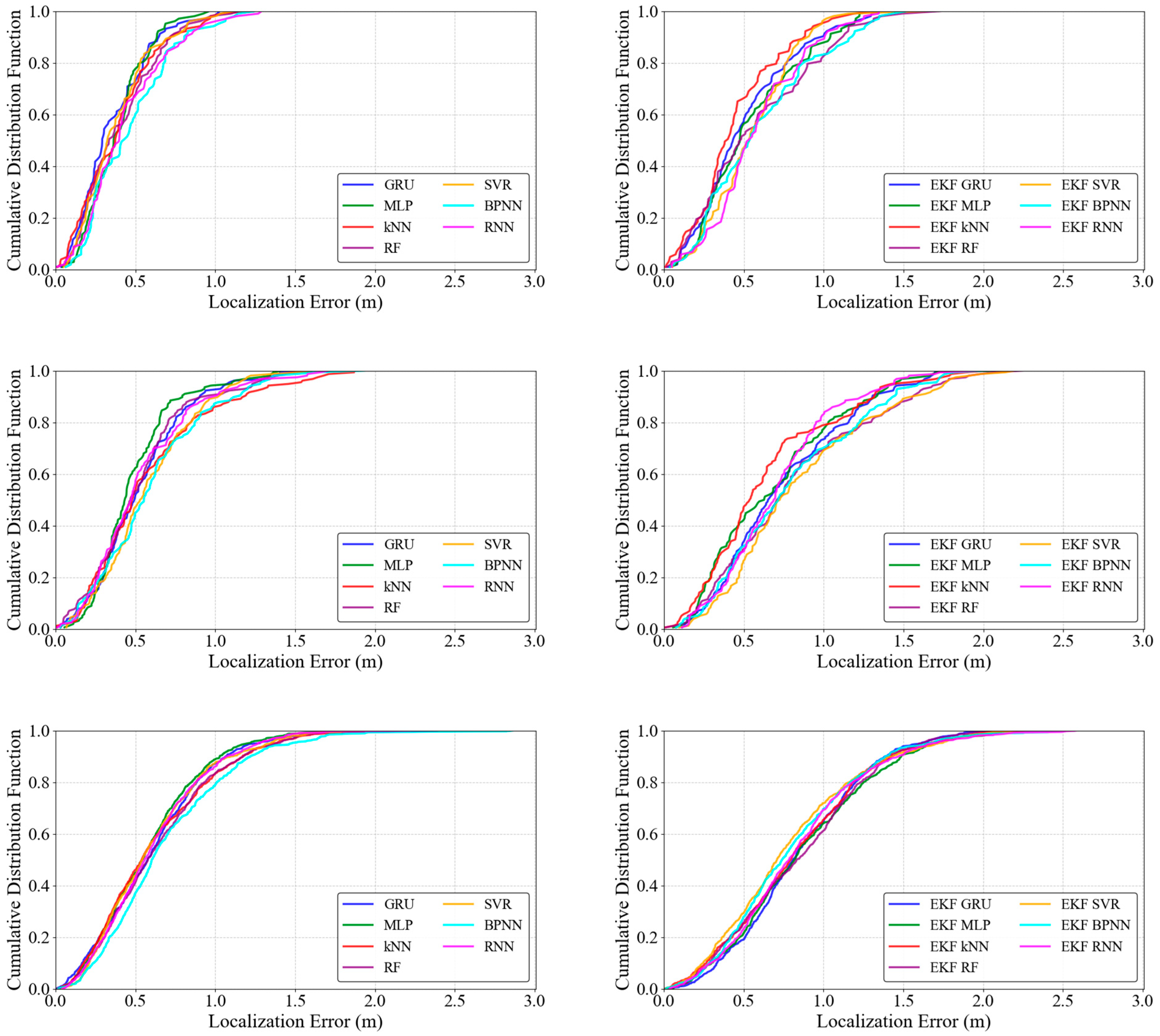
5.3. Accuracy Results

By utilizing the obtained radio maps of the experimental area and the various routes, the coordinates of the robot will be predicted using the ML methods outlined in Section 3.4. The prediction results of the models are evaluated using the coefficient of determination R² for each method outlined in Section 3.2.

Table 2. Model Accuracy Results for ML.

ML	Scenario	EKF	No Filter	Sector_256	Sector_1024
GRU	First	0.8598	0.9298	0.9454	0.9354
	Second	0.7324	0.8595	0.9102	0.8902
	Third	0.4799	0.7152	0.8512	0.8412
MLP	First	0.8440	0.9282	0.9010	0.8810
	Second	0.7593	0.8848	0.8920	0.8720
	Third	0.4301	0.7418	0.8413	0.8213
KNN	First	0.8899	0.9151	0.8708	0.8608
	Second	0.7694	0.8093	0.8491	0.8321
	Third	0.4773	0.6893	0.8012	0.8129
RF	First	0.8125	0.9134	0.8394	0.8235
	Second	0.6611	0.8560	0.8723	0.8456
	Third	0.4692	0.6805	0.7984	0.7754
SVR	First	0.8529	0.9218	0.9032	0.8976
	Second	0.6484	0.8382	0.8566	0.8487
	Third	0.5247	0.7167	0.7712	0.7885
BPNN	First	0.8068	0.8330	0.8983	0.8912
	Second	0.6940	0.8195	0.8117	0.7862
	Third	0.5462	0.5318	0.7641	0.7510
RNN	First	0.8310	0.8957	0.9200	0.9230
	Second	0.7620	0.8497	0.8579	0.8283
	Third	0.4946	0.7212	0.7639	0. 8165

presents the ML results as R² scores for three scenarios, using different preprocessing methods and configurations. The GRU method combined with the Sector_256 configuration achieves the highest accuracy across all models and scenarios. This indicates that the GRU’s recurrent architecture is particularly effective for mobile node localization in wireless sensor networks, likely due to its ability to retain long-term dependencies, such as past RSSI measurements. Additionally, it can be concluded that the proposed sectorization method enhances prediction accuracy. For example, the GRU model achieves the highest R² scores of 0.9454 in the first scenario, 0.9102 in the second, and 0.8512 in the third when using the Sector_256 configuration.

The 1024-sector division method shows solid results: 0.9354 in the first scenario, 0.8902 in the second, and 0.8412 in the third. Although Sector_256 outperformed Sector_1024, it can be anticipated that the localization accuracy will improve with Sector_1024, as a greater number of sectors enables more precise positioning of the nodes. The ML results further suggest that the application of the EKF for preprocessing does not yield significant improvements compared to models trained without the filter. This is likely to be due to the dynamic fluctuations in RSSI values caused by the movement of the mobile node. Figure 14 visualizes the performance of the ML models using bar charts, providing a clearer comparison of their accuracy across the scenarios.

Figure 15, Figure 16 and Figure 17 present the machine learning results using MAE and RMSE metrics for the first, second, and third scenarios, respectively. The X-axis represents the sequential position numbers traversed by the mobile robot. The first scenario includes 104 points, the second 157 points, and the third 736 points. From the analysis of the graphs, it can be concluded that the GRU and MLP models deliver the best performance compared to other ML models.

For the first scenario, the best performing models are GRU, achieving an average mean absolute error of 0.246 m and a root mean square error of 0.300 m, and SVR, with an average mean absolute error of 0.253 m and a root mean square error of 0.315 m. The worst model is BPNN, which has an average mean absolute error of 0.316 m and a root mean square error of 0.378 m.

For the second scenario, GRU and MLP deliver the best results. GRU achieves an average mean absolute error of 0.310 m and a root mean square error of 0.427 m, while MLP demonstrates slightly better performance in terms of root mean square error at 0.393 m. The worst model in this scenario is BPNN, with an average mean absolute error of 0.387 m and a root mean square error of 0.492 m.

For the third scenario, GRU and MLP again perform best, with GRU achieving an average mean absolute error of 0.376 m and a root mean square error of 0.499 m, while MLP records an average mean absolute error of 0.377 m and a root mean square error of 0.475 m. The worst model is BPNN, which has an average mean absolute error of 0.447 m and a root mean square error of 0.569 m. Overall, the localization accuracy for the third scenario was not very high because the number of points obtained from RSSI values in the first and second scenarios is significantly lower than in the third. Consequently, in the third scenario, where the mobile robot follows a sinusoidal trajectory with high amplitude and frequency, odometry errors accumulate faster, leading to a noticeable decrease in localization accuracy.

It is also evident that models incorporating the Kalman filter perform worse than those without the filter.

Figure 18 presents the cumulative distribution of absolute errors (AE) by distance for various models across different scenarios. The left column shows the CDF results for the first, second, and third test scenarios, respectively. In all scenarios, the GRU and MLP models exhibit lower absolute error values, especially at shorter distances. However, when applying the EKF (shown in the right column), the absolute error increases slightly for each scenario, indicating that EKF performs poorly in this context.

The MLP model shows a pattern of increasing AE across scenarios, with values of 0.396 m, 0.546 m, and 0.621 m for the first, second, and third scenarios, respectively. The kNN model achieves competitive results without EKF, with an AE of 0.390 m for the first scenario, 0.587 m for the second, and 0.640 m for the third. Other models such as RF and SVR follow this trend, where the average AE remains lower in the absence of EKF. For example, RF achieves AE values of 0.402 m, 0.553 m, and 0.641 m without EKF, but slightly higher values with the filter applied. The RNN and BPNN models also reflect these patterns. Without the filter, RNN achieves AE values of 0.441 m, 0.557 m, and 0.639 m across the three scenarios, showing a moderate increase as the trajectory complexity increases. BPNN, however, exhibits the highest errors among the tested models, with AE values of 0.467 m, 0.598 m, and 0.693 m without EKF. These results indicate the relatively weaker capabilities of BPNN compared to GRU, MLP, and kNN. The cumulative distribution of localization errors (CDF) highlights that GRU and MLP maintain a significant proportion of errors below 0.5 m for shorter trajectories, demonstrating their robustness in simpler scenarios. However, as trajectory complexity increases, the AE and error spread increase for all models. This is because, in the first and second scenarios, the number of points derived from the RSSI values is significantly lower than in the third. Consequently, in the third scenario, where the mobile robot follows a sinusoidal trajectory with high amplitude and frequency, the odometry errors accumulate, leading to a noticeable decrease in localization accuracy.

Overall, GRU and MLP stand out as the most robust models in all scenarios, achieving the lowest AE values. This indicates their suitability for trajectory prediction tasks, especially in cases involving moderate trajectory complexity.

For the best GRU model, the AE gradually increases from the first to the third scenario (0.384 m for the first, 0.542 m for the second, and 0.611 m for the third), suggesting that the models struggle with more complex trajectories.

6. Discussion

During the literature review in the field of indoor LoRa mobile node localization research, we found that the problem of mobile node localization, especially in dynamic environments, remains an under-explored area, despite the availability of many solutions for static nodes. In [38], a deep autoencoder method was proposed to handle missing data and outliers using artificial neural network (ANN), long short-term memory (LSTM) and convolutional neural network (CNN) to predict the location based on RSSI fingerprints. An average error of 1.27 m was achieved in static environments with data splits of 70% and 30% for training and testing, respectively. In [35], an improved method based on random forest (RF) and particle swarm algorithm (PSO) was proposed, which uses a new RSSI RANGE parameter, achieving the best accuracy of 0.82 m by filtering the data. In [37], the authors presented a random neural network (RNN)-based indoor localization system based on RSSI measurement, which achieved an average error of 0.12 m. Although this model demonstrated excellent results in their study, in our case with dynamic data collection for mobile nodes, its performance was lower, with an average localization error of 0.441 m for the best RNN model. A back-propagation neural network [BPNN]-based model with an outlier removal filter during data collection [36] achieved an average error of 0.5971 m indoors. While this approach showed promising results in their study, in our scenario, with dynamic data collection, BPNN performed worse, achieving an average localization error of 0.467 m. However, the environmental dynamics of moving objects is still not considered and is included by [41] for future implementation of mobile node position prediction. In traditional trilateration methods [32], experimental results show that LoRa localization can achieve an accuracy better than 1.6 m under line-of-sight conditions. In [62], four wireless technologies for indoor localization were compared: Wi-Fi, Bluetooth, Zigbee, and LoRa, and LoRa achieved an accuracy of 0.846 m under very noisy environments and 1.534 m under low noise conditions. In all the above works, the localization problem is solved for static nodes. Radio maps were obtained by repeatedly measuring RSSI at junctions of a predefined grid in a room.

The results obtained in our work are comparable with the results obtained in [63,64] using Wi-Fi and Zigbee, since these works considered mobile wireless nodes. In [63], two important methods are used to ensure accurate indoor localization based on collecting Wi-Fi RSSI fingerprints: the Support Vector Machine (SVM) and Long-Short Term Memory (LSTM) machine learning algorithms. As a result, the average error in the algorithm with LSTM is 0.9 m, with SVM it is 1.1 m. In [64], an adaptive wireless indoor localization system (ILS) for a dynamic environment was proposed, which includes an automated database update process and a new Adaptive signal model fingerprinting (ASMF) algorithm.

Table 3. Comparative analysis of technologies for localization of mobile nodes.

Paper	Method	Machine Learning	Localization Error	WSN
[38]	Fingerprint	ANN, LSTM, CNN	1.27 m	LoRa
[36]	Fingerprint	BPNN (Back-Propagation Neural Network)	0.5971 m	LoRa
[35]	Fingerprint	RF	0.82 m	LoRa
[36]	Fingerprint	RNN	0.12 m	LoRa
[32]	Trilateration	N/A	1.6 m	LoRa
[62]	Trilateration	N/A	0.846 m and 1.534 m	LoRa
[63]	Fingerprint	LSTM, SVM	0.9 m and 1.1 m	Wi-Fi
[64]	Adaptive signal model fingerprinting (ASMF)	kNN	0.712 m and 0.939 m	Zigbee
Proposed research	Fingerprint	GRU, MLP, kNN, RF, SVR, BPNN and RNN	0.384 m	LoRa

shows the numerical results of the above works.

In our study, the best GRU model achieved an average localization error of 0.384 m and the average absolute localization error of 0.246 m were achieved, which is a good result under multiple reflection conditions in the room.

The proposed method of dividing into sectors showed better results in comparison with other works. It allows speeding up of the process of obtaining a radio map and increasing the accuracy of localization of mobile nodes using LoRa technology.

7. Conclusions

As a result of the study, a new method for localizing LoRa mobile wireless nodes indoors with division into sectors was proposed. The use of the extended Kalman filter (EKF) for localizing mobile wireless nodes indoors does not provide significant improvements. The new method of dividing into sectors minimizes the impact of noise and nonlinearity of signal propagation. In addition, in this work, the test sample and training sample data were not parts of the same dataset, which increases the validity of the results and the purity of the experiment.

The best results were shown by GRU with division into 256 sectors with an accuracy of 94.54% for the first scenario, 91.02% for the second scenario and 85.12% for the third scenario. The method based on division into 1024 sectors also shows good results using GRU: the first scenario—93.54%, the second—89.02%, the third—84.12%. The cumulative error distribution function analysis showed that the average localization error was 0.384 m, and the average absolute localization error was 0.246 m, which is a good result in indoor multiple reflection conditions.

As part of our future work, we plan to focus on real-time node localization to en-hance the system’s applicability and provide a real-time estimation, expand the experimental area, and explore hybrid approaches for more accurate localization of mobile nodes.

References

1. Dritsas, E.; Trigka, M. Machine Learning for Blockchain and IoT Systems in Smart Cities: A Survey. Future Internet 2024, 16, 324. [Google Scholar] [CrossRef]
2. Umetani, T.; Kondo, Y.; Tokuda, T. Rapid Development of a Mobile Robot for the Nakanoshima Challenge Using a Robot for Intelligent Environments. J. Robot. Mechatron. 2020, 32, 1211–1218. [Google Scholar] [CrossRef]
3. Fath, A.; Hanna, N.; Liu, Y.; Tanch, S.; Xia, T.; Huston, D. Indoor Infrastructure Maintenance Framework Using Networked Sensors, Robots, and Augmented Reality Human Interface. Future Internet 2024, 16, 170. [Google Scholar] [CrossRef]
4. Shit, R.C.; Sharma, S.; Puthal, D.; Zomaya, A.Y. Location of Things (LoT): A Review and Taxonomy of Sensors Localization in IoT Infrastructure. IEEE Commun. Surv. Tutor. 2018, 20, 2028–2061. [Google Scholar] [CrossRef]
5. Kang, J.M.; Yoon, T.S.; Kim, E.; Park, J.B. Lane-Level Map-Matching Method for Vehicle Localization Using GPS and Camera on a High-Definition Map. Sensors 2020, 20, 2166. [Google Scholar] [CrossRef]
6. Janssen, T.; Koppert, A.; Berkvens, R.; Weyn, M. A survey on IoT positioning leveraging LPWAN, GNSS, and LEO-PNT. IEEE Internet Things J. 2023, 10, 11135–11159. [Google Scholar] [CrossRef]
7. Florio, A.; Bnilam, N.; Talarico, C.; Crosta, P.; Avitabile, G.; Coviello, G. LEO-Based Coarse Positioning Through Angle-of-Arrival Estimation of Signals of Opportunity. IEEE Access 2024, 12, 17446–17459. [Google Scholar] [CrossRef]
8. Pascacio, P.; Casteleyn, S.; Torres-Sospedra, J.; Lohan, E.S.; Nurmi, J. Collaborative Indoor Positioning Systems: A Systematic Review. Sensors 2021, 21, 1002. [Google Scholar] [CrossRef] [PubMed]
9. Ngamakeur, K.; Yongchareon, S.; Yu, J.; Islam, S. Passive infrared sensor dataset and deep learning models for device-free indoor localization and tracking. Pervasive Mob. Comput. 2023, 88, 101721. [Google Scholar] [CrossRef]
10. Huang, Y.-H.; Lin, C.-T. Indoor Localization Method for a Mobile Robot Using LiDAR and a Dual AprilTag. Electronics 2023, 12, 1023. [Google Scholar] [CrossRef]
11. Do, T.-H.; Yoo, M. An in-Depth Survey of Visible Light Communication Based Positioning Systems. Sensors 2016, 16, 678. [Google Scholar] [CrossRef] [PubMed]
12. Wang, R.; Niu, G.; Cao, Q.; Chen, C.S.; Ho, S.-W. A Survey of Visible-Light-Communication-Based Indoor Positioning Systems. Sensors 2024, 24, 5197. [Google Scholar] [CrossRef]
13. Wu, J.; Yang, T.; Zhang, Z. Research on Wi-Fi Fingerprint Database Construction Method Based on Environmental Feature Awareness. Appl. Syst. Innov. 2024, 7, 99. [Google Scholar] [CrossRef]
14. Fontaine, J.; Van Herbruggen, B.; Shahid, A.; Kram, S.; Stahlke, M.; De Poorter, E. Ultra Wideband (UWB) Localization Using Active CIR-Based Fingerprinting. IEEE Commun. Lett. 2023, 27, 1322–1326. [Google Scholar] [CrossRef]
15. Ahmed, H.M.; Rashid, A.N. Rfid indoor localization based received signal strength. In Proceedings of the 2021 14th International Conference on Developments in eSystems Engineering (DeSE), Sharjah, United Arab Emirates, 7–10 December 2021; pp. 590–593. [Google Scholar] [CrossRef]
16. Al Mojamed, M. On the Use of LoRaWAN for Mobile Internet of Things: The Impact of Mobility. Appl. Syst. Innov. 2022, 5, 5. [Google Scholar] [CrossRef]
17. Fahama, H.; Ansari-Asl, K.; Kavian, Y.S.; Soorki, M.N. An Experimental Comparison of RSSI-Based Indoor Localization Techniques Using ZigBee Technology. IEEE Access 2023, 11, 87985–87996. [Google Scholar] [CrossRef]
18. Asaad, S.M.; Maghdid, H.S. A comprehensive review of indoor/outdoor localization solutions in IoT era: Research challenges and future perspectives. Comput. Netw. 2022, 212, 109041. [Google Scholar] [CrossRef]
19. Zafari, F.; Gkelias, A.; Leung, K.K. A survey of indoor localization systems and technologies. IEEE Commun. Surv. Tutor. 2019, 21, 2568–2599. [Google Scholar] [CrossRef]
20. Islam, B.; Islam, M.T.; Kaur, J.; Nirjon, S. Lorain: Making a case for lora in indoor localization. In Proceedings of the 2019 IEEE International Conference on Pervasive Computing and Communications Workshops (PerCom Workshops), Kyoto, Japan, 11–15 March 2019. [Google Scholar] [CrossRef]
21. Tomic, S.; Beko, M.; Dinis, R. RSS-AoA-Based Target Localization and Tracking in Wireless Sensor Networks; River Publishers: New York, NY, USA, 2022. [Google Scholar] [CrossRef]
22. Yuan, W.; Wu, N.; Guo, Q.; Huang, X.; Li, Y.; Hanzo, L. TOA-based passive localization constructed over factor graphs: A unified framework. IEEE Trans. Commun. 2019, 67, 6952–6965. [Google Scholar] [CrossRef]
23. Antonello, F.; Avitabile, G.; Coviello, G. Digital phase estimation through an I/Q approach for angle of arrival full-hardware localization. In Proceedings of the 2020 IEEE Asia Pacific Conference on Circuits and Systems (APCCAS), Ha Long, Vietnam, 8–10 December 2020. [Google Scholar] [CrossRef]
24. Florio, A.; Avitabile, G.; Coviello, G. A Linear Technique for Artifacts Correction and Compensation in Phase Interferometric Angle of Arrival Estimation. Sensors 2022, 22, 1427. [Google Scholar] [CrossRef] [PubMed]
25. Yiu, S.; Dashti, M.; Claussen, H.; Perez-Cruz, F. Wireless RSSI Fingerprinting Localization. Signal Process. 2017, 131, 235–244. [Google Scholar] [CrossRef]
26. Nessa, A.; Adhikari, B.; Hussain, F.; Fernando, X. A Survey of Machine Learning for Indoor Positioning. IEEE Access 2020, 8, 214945–214965. [Google Scholar] [CrossRef]
27. Khan, I.M.; Thompson, A.; Al-Hourani, A.; Sithamparanathan, K.; Rowe, W.S.T. RSSI and Device Pose Fusion for Fingerprinting-Based Indoor Smartphone Localization Systems. Future Internet 2023, 15, 220. [Google Scholar] [CrossRef]
28. Kumar, P.; Reddy, L.; Varma, S. Distance measurement and error estimation scheme for RSSI based localization in wireless sensor networks. In Proceedings of the 2009 Fifth International Conference on Wireless Communication and Sensor Networks (WCSN), Allahabad, India, 15–19 December 2009; pp. 1–4. [Google Scholar] [CrossRef]
29. Yang, B.; Jia, X.; Yang, F. Variational Bayesian Adaptive Unscented Kalman Filter for RSSI-Based Indoor Localization. Int. J. Control Autom. Syst. 2021, 19, 1183–1193. [Google Scholar] [CrossRef]
30. Potortì, F.; Park, S.; Jiménez Ruiz, A.R.; Barsocchi, P.; Girolami, M.; Crivello, A.; Lee, S.Y.; Lim, J.H.; Torres-Sospedra, J.; Seco, F.; et al. Comparing the Performance of Indoor Localization Systems through the EvAAL Framework. Sensors 2017, 17, 2327. [Google Scholar] [CrossRef] [PubMed]
31. Mangalvedhe, N.; Ratasuk, R.; Ghosh, A. NB-IoT deployment study for low power wide area cellular IoT. In Proceedings of the 2016 IEEE 27th Annual International Symposium on Personal, Indoor, and Mobile Radio Communications (PIMRC), Valencia, Spain, 4–8 September 2016; pp. 1–6. [Google Scholar] [CrossRef]
32. Kim, K.; Li, S.; Heydariaan, M.; Smaoui, N.; Gnawali, O.; Suh, W.; Suh, M.J.; Kim, J.I. Feasibility of LoRa for Smart Home Indoor Localization. Appl. Sci. 2021, 11, 415. [Google Scholar] [CrossRef]
33. Chen, H.; Yang, J.; Hao, Z.; Qi, T.; Liu, T. Research on indoor multi-floor positioning method based on LoRa. Comput. Netw. 2024, 254, 110838. [Google Scholar] [CrossRef]
34. Anjum, M.; Khan, M.A.; Hassan, S.A.; Mahmood, A.; Qureshi, H.K.; Gidlund, M. RSSI fingerprinting-based localization using machine learning in LoRa networks. IEEE Internet Things Mag. 2020, 3, 53–59. [Google Scholar] [CrossRef]
35. Chen, H.; Yang, J.; Hao, Z.; Ga, M.; Han, X.; Zhang, X.; Chen, Z. Research on indoor positioning method based on LoRa-improved fingerprint localization algorithm. Sci. Rep. 2023, 13, 13981. [Google Scholar] [CrossRef]
36. Lu, K.; Yue, Y.; Ma, J. Enhanced LoRaWAN RSSI indoor localization based on BP neural network. In Proceedings of the 2021 IEEE 4th International Conference on Information Systems and Computer Aided Education (ICISCAE), Dalian, China, 24–26 September 2021; pp. 190–195. [Google Scholar] [CrossRef]
37. Ingabire, W.; Larijani, H.; Gibson, R.M.; Qureshi, A.-U.-H. LoRaWAN Based Indoor Localization Using Random Neural Networks. Information 2022, 13, 303. [Google Scholar] [CrossRef]
38. Purohit, J.; Wang, X.; Mao, S.; Sun, X.; Yang, C. Fingerprinting-based indoor and outdoor localization with LoRa and deep learning. In Proceedings of the GLOBECOM 2020—2020 IEEE Global Communications Conference, Taipei, Taiwan, 7–11 December 2020; pp. 1–6. [Google Scholar] [CrossRef]
39. Suroso, D.J.; Rudianto, A.S.; Arifin, M.; Hawibowo, S. Random forest and interpolation techniques for fingerprint-based indoor positioning system in un-ideal Environment. Int. J. Comput. Digit. Syst. 2021, 10, 701–713. [Google Scholar] [CrossRef] [PubMed]
40. Perković, T.; Dujić Rodić, L.; Šabić, J.; Šolić, P. Machine Learning Approach towards LoRaWAN Indoor Localization. Electronics 2023, 12, 457. [Google Scholar] [CrossRef]
41. Ali, I.T.; Muis, A.; Sari, R.F. A deep learning model implementation based on rssi fingerprinting for lora-based indoor localization. EUREKA Phys. Eng. 2021, 1, 40–59. [Google Scholar] [CrossRef]
42. Zhu, H.; Tsang, K.F.; Liu, Y.; Wei, Y.; Wang, H.; Wu, C.K.; Chi, H.R. Extreme RSS based indoor localization for LoRaWAN with boundary autocorrelation. IEEE Trans. Ind. Inform. 2020, 17, 4458–4468. [Google Scholar] [CrossRef]
43. Seller, O.B.; Sornin, N. Low Power Long Range Transmitter. U.S. Patent No. 9,252,834, 2 February 2016. [Google Scholar]
44. de Carvalho Silva, J.; Rodrigues, J.J.; Alberti, A.M.; Solic, P.; Aquino, A.L. LoRaWAN—A low power WAN protocol for Internet of Things: A review and opportunities. In Proceedings of the 2017 2nd International Multidisciplinary Conference on Computer and Energy Science (SpliTech), Split, Croatia, 12–14 July 2017; pp. 1–6. [Google Scholar]
45. Coutinho, M.; Afonso, J.A.; Lopes, S.F. An Efficient Adaptive Data-Link-Layer Architecture for LoRa Networks. Future Internet 2023, 15, 273. [Google Scholar] [CrossRef]
46. Ayele, E.D.; Hakkenberg, C.; Meijers, J.P.; Zhang, K.; Meratnia, N.; Havinga, P.J. Performance analysis of LoRa radio for an indoor IoT applications. In Proceedings of the 2017 International Conference on Internet of Things for the Global Community (IoTGC), Funchal, Portugal, 10–13 July 2017; pp. 1–8. [Google Scholar] [CrossRef]
47. Anjum, M.; Khan, M.A.; Hassan, S.A.; Mahmood, A.; Gidlund, M. Analysis of RSSI fingerprinting in LoRa networks. In Proceedings of the 2019 15th International Wireless Communications & Mobile Computing Conference (IWCMC), Tangier, Morocco, 24–28 June 2019; pp. 1178–1183. [Google Scholar] [CrossRef]
48. Raghav, R.S.; Thirugnanasambandam, K.; Varadarajan, V.; Vairavasundaram, S.; Ravi, L. Artificial Bee Colony reinforced extended Kalman filter localization algorithm in internet of things with big data blending technique for finding the accurate position of reference nodes. Big Data 2022, 10, 186–203. [Google Scholar] [CrossRef] [PubMed]
49. Venkatesh, R.; Mittal, V.; Tammana, H. Indoor localization in BLE using mean and median filtered RSSI values. In Proceedings of the 2021 5th International Conference on Trends in Electronics and Informatics (ICOEI), Tirunelveli, India, 3–5 June 2021; pp. 227–234. [Google Scholar] [CrossRef]
50. Aydin, H.M.; Ali, M.A.; Soyak, E.G. The analysis of feature selection with machine learning for indoor positioning. In Proceedings of the 2021 29th Signal Processing and Communications Applications Conference (SIU), Istanbul, Turkey, 9–11 June 2021; pp. 1–4. [Google Scholar] [CrossRef]
51. Pak, J.M. Switching Extended Kalman Filter Bank for Indoor Localization Using Wireless Sensor Networks. Electronics 2021, 10, 718. [Google Scholar] [CrossRef]
52. Schölkopf, B. Learning with Kernels: Support Vector Machines, Regularization, Optimization, and Beyond; MIT Press: Cambridge, MA, USA, 2002. [Google Scholar]
53. Song, Y.; Liang, J.; Lu, J.; Zhao, X. An efficient instance selection algorithm for k nearest neighbor regression. Neurocomputing 2017, 251, 26–34. [Google Scholar] [CrossRef]
54. Devroye, L. The uniform convergence of nearest neighbor regression function estimators and their application in optimization. IEEE Trans. Inf. Theory 1978, 24, 142–151. [Google Scholar] [CrossRef]
55. Breiman, L. Random forests. Mach. Learn. 2001, 45, 5–32. [Google Scholar] [CrossRef]
56. Pinkus, A. Approximation theory of the MLP model in neural networks. Acta Numer. 1999, 8, 143–195. [Google Scholar] [CrossRef]
57. Chung, J.; Gulcehre, C.; Cho, K.; Bengio, Y. Empirical evaluation of gated recurrent neural networks on sequence modeling. arXiv 2014, arXiv:1412.3555. [Google Scholar] [CrossRef]
58. Rumelhart, D.E.; Hinton, G.E.; Williams, R.J. Learning representations by back-propagating errors. Nature 1986, 323, 533–536. [Google Scholar] [CrossRef]
59. Gelenbe, E. Random neural networks with negative and positive signals and product form solution. Neural Comput. 1989, 1, 502–510. [Google Scholar] [CrossRef]
60. Available online: https://emanual.robotis.com/docs/en/platform/turtlebot3/overview/ (accessed on 25 November 2024).
61. Available online: https://www.dragino.com/products/lora/item/231-la66-lorawan-shield.html (accessed on 25 November 2024).
62. Sadowski, S.; Spachos, P. Rssi-based indoor localization with the internet of things. IEEE Access 2018, 6, 30149–30161. [Google Scholar] [CrossRef]
63. Abbas, H.A.; Boskany, N.W.; Ghafoor, K.Z.; Rawat, D.B. Wi-Fi based accurate indoor localization system using SVM and LSTM algorithms. In Proceedings of the 2021 IEEE 22nd International Conference on Information Reuse and Integration for Data Science (IRI), Las Vegas, NV, USA, 10–12 August 2021; pp. 416–422. [Google Scholar] [CrossRef]
64. Luo, R.C.; Hsiao, T.J. Dynamic wireless indoor localization incorporating with an autonomous mobile robot based on an adaptive signal model fingerprinting approach. IEEE Trans. Ind. Electron. 2018, 66, 1940–1951. [Google Scholar] [CrossRef]
Figure 1. The LoRaWAN network architecture.
Futureinternet 16 00450 g001
Figure 2. Research map.
Futureinternet 16 00450 g002
Figure 3. Division of the experimental area into 256 (a) and 1024 (b) sectors.
Futureinternet 16 00450 g003
Figure 4. MLP architecture.
Futureinternet 16 00450 g004
Figure 5. The Gated Recurrent Unit architecture.
Futureinternet 16 00450 g005
Figure 6. Experimental setup.
Futureinternet 16 00450 g006
Figure 7. LoRaWAN data collection devices: (A) TurtleBot3 mobile robot, LoRaWAN LA66 Shield (B) and LoRaWAN USB Adapter (C).
Futureinternet 16 00450 g007
Figure 8. The movement trajectory for collecting training data.
Futureinternet 16 00450 g008
Figure 9. Three scenarios of robot movement: (a) first scenario (b) second scenario (c) third scenario.
Futureinternet 16 00450 g009
Figure 10. Received radio maps: (a) General radio map (b) First scenario (c) Second scenario (d) Third scenario.
Futureinternet 16 00450 g010aFutureinternet 16 00450 g010b
Figure 11. Application of the EKF for data smoothing: (a) first, (b) second, (c) third, (d) fourth receiver.
Futureinternet 16 00450 g011aFutureinternet 16 00450 g011b
Figure 12. Radio map after applying the EKF.
Futureinternet 16 00450 g012
Figure 13. Radio map after applying the sectorization method. (ad)—for the first, second, third, and fourth receivers with 256 sectors, respectively. (eh)—for the first, second, third, and fourth receivers with 1024 sectors, respectively.
Futureinternet 16 00450 g013aFutureinternet 16 00450 g013b
Figure 14. ML results (R2 score) for various types of routes: (a) first (b) second (c) third.
Futureinternet 16 00450 g014
Figure 15. ML results for the first scenario: (a) MAE, (b) RMSE.
Futureinternet 16 00450 g015
Figure 16. ML results for the second scenario: (a) MAE, (b) RMSE.
Futureinternet 16 00450 g016
Figure 17. ML results for the third scenario: (a) MAE, (b) RMSE.
Futureinternet 16 00450 g017
Figure 18. Cumulative distribution of average localization errors.
Futureinternet 16 00450 g018