Article

Nonlinear Dynamics and Machine Learning for Robotic Control Systems in IoT Applications

by
Vesna Antoska Knights
1,*,
Olivera Petrovska
2 and
Jasenka Gajdoš Kljusurić
3
1
Faculty of Technology and Technical Sciences, University St. Kliment Ohridski, 7000 Bitola, North Macedonia
2
Faculty of Technical Science, Mother Teresa University, 1000 Skopje, North Macedonia
3
Faculty of Food Technology and Biotechnology, University of Zagreb, Pierottijeva 6, 10000 Zagreb, Croatia
*
Author to whom correspondence should be addressed.
Future Internet 2024, 16(12), 435; https://doi.org/10.3390/fi16120435
Submission received: 9 October 2024 / Revised: 14 November 2024 / Accepted: 18 November 2024 / Published: 21 November 2024
(This article belongs to the Special Issue Machine Learning for Blockchain and IoT Systems in Smart City)

Abstract

:
This paper presents a novel approach to robotic control by integrating nonlinear dynamics with machine learning (ML) in an Internet of Things (IoT) framework. This study addresses the increasing need for adaptable, real-time control systems capable of handling complex, nonlinear dynamic environments and the importance of machine learning. The proposed hybrid control system is designed for a 20 degrees of freedom (DOFs) robotic platform, combining traditional nonlinear control methods with machine learning models to predict and optimize robotic movements. The machine learning models, including neural networks, are trained using historical data and real-time sensor inputs to dynamically adjust the control parameters. Through simulations, the system demonstrated improved accuracy in trajectory tracking and adaptability, particularly in nonlinear and time-varying environments. The results show that combining traditional control strategies with machine learning significantly enhances the robot’s performance in real-world scenarios. This work offers a foundation for future research into intelligent control systems, with broader implications for industrial applications where precision and adaptability are critical.

1. Introduction

The integration of robotic systems with advanced control methods and machine learning has become a key research focus, particularly in the context of the Internet of Things (IoT) [1,2]. As IoT applications continue to expand across various industries [3,4], from smart agriculture to autonomous transportation [5,6], the demand for adaptive, real-time control systems that can handle complex, dynamic environments has grown significantly [7]. These systems must be capable of interacting with diverse sensors, processing vast amounts of data, and making intelligent decisions to optimize performance [8]. In this regard, the combination of nonlinear dynamics, machine learning, and IoT technologies offers a promising approach [9,10].
Nonlinear control systems are well-suited for managing the complex dynamics of robotic platforms, especially those with multiple degrees of freedom [11,12]. Traditional control techniques, such as PID and adaptive control, have been widely applied in robotics [13]. However, these approaches often struggle in environments characterized by high nonlinearity, uncertainty, and time-varying conditions. Recent advancements in machine learning, particularly deep learning and recurrent neural networks, provide new opportunities to enhance control accuracy and adaptability [14,15,16,17]. By leveraging the universal approximation capability of neural networks, it is possible to model the intricate relationships between input control signals and system behavior, enabling more precise control in real-time scenarios [17].
In parallel, the integration of the IoT allows for the seamless exchange of information between robotic systems and distributed networks, facilitating real-time monitoring, control, and decision-making across large-scale environments [18,19].
The IoT infrastructure supports the collection of sensor [20,21,22] data from various sources, which can be fed into machine learning models for the continuous adaptation of control parameters. This adaptability is essential in applications such as smart farming, where environmental conditions can change unpredictably, requiring the control system to respond promptly.
This paper introduces a hybrid control architecture that combines nonlinear dynamics and machine learning (ML) techniques to optimize robotic control systems, specifically designed for a 20 degrees of freedom (DOFs) robotic platform [23]. The integration of ML into this system enables real-time adjustments, improving the adaptability and precision of the control strategy.
This research builds on previous work by integrating nonlinear dynamic modeling with machine learning and the IoT, focusing on practical implementation and real-time adaptability in various IoT-driven scenarios [24,25,26,27,28,29,30,31].
Recent studies have demonstrated the potential of machine learning techniques in robotic control. For instance, El-Hussieny et al. [11] utilized a deep learning-based Model Predictive Control (MPC) framework to enhance the trajectory tracking of a three DOFs robotic leg, highlighting the advantages of data-driven models over traditional analytical methods in real-time control scenarios. Similarly, Yuan et al. [24] explored the application of auxiliary physics-informed neural networks to solving the forward and inverse problems of nonlinear integro-differential equations, demonstrating the efficacy of adaptive learning models in complex environments. Chen and Wen [32] explored the application of multi-layer neural networks in industrial robot trajectory tracking, while Li et al. [33] and Zheng et al. [34] applied recurrent neural networks to trajectory tracking for high-dimensional robotic systems, demonstrating the efficacy of adaptive learning models in complex environments. Moreover, the integration of the IoT with robotic control systems has been discussed extensively, particularly in smart farming applications [35,36,37] where real-time data processing and environmental adaptability are crucial.
The diagram in Figure 1 illustrates the four-layer architecture of an IoT system [38], with each layer serving specific functions in the IoT ecosystem:
Sensing layer: This layer showcases the use of embedded devices, such as sensors and actuators, tasked with data acquisition. These devices collect environmental data.
Network layer: This employs a range of communication technologies including WiFi and Bluetooth for local connectivity. For applications requiring extended range, technologies like Zigbee, cellular networks (4G/5G), and LoRaWAN are also incorporated. This layer may also integrate security measures such as encryption and authentication to safeguard data exchanges.
Data processing layer: Located primarily in cloud-based platforms, this layer handles the heavy lifting of data analysis. It processes incoming data streams to extract actionable insights and supports advanced computational tasks. Technologies in use include data management systems and machine learning algorithms, often within structures like data lakes that store vast amounts of unprocessed data.
Application layer: This is a simulator that control applications and highlights where the data become actionable through various applications. It is potentially developed in programming environments like MATLAB R2024a, Python 3.10, or Java 19.0.1.

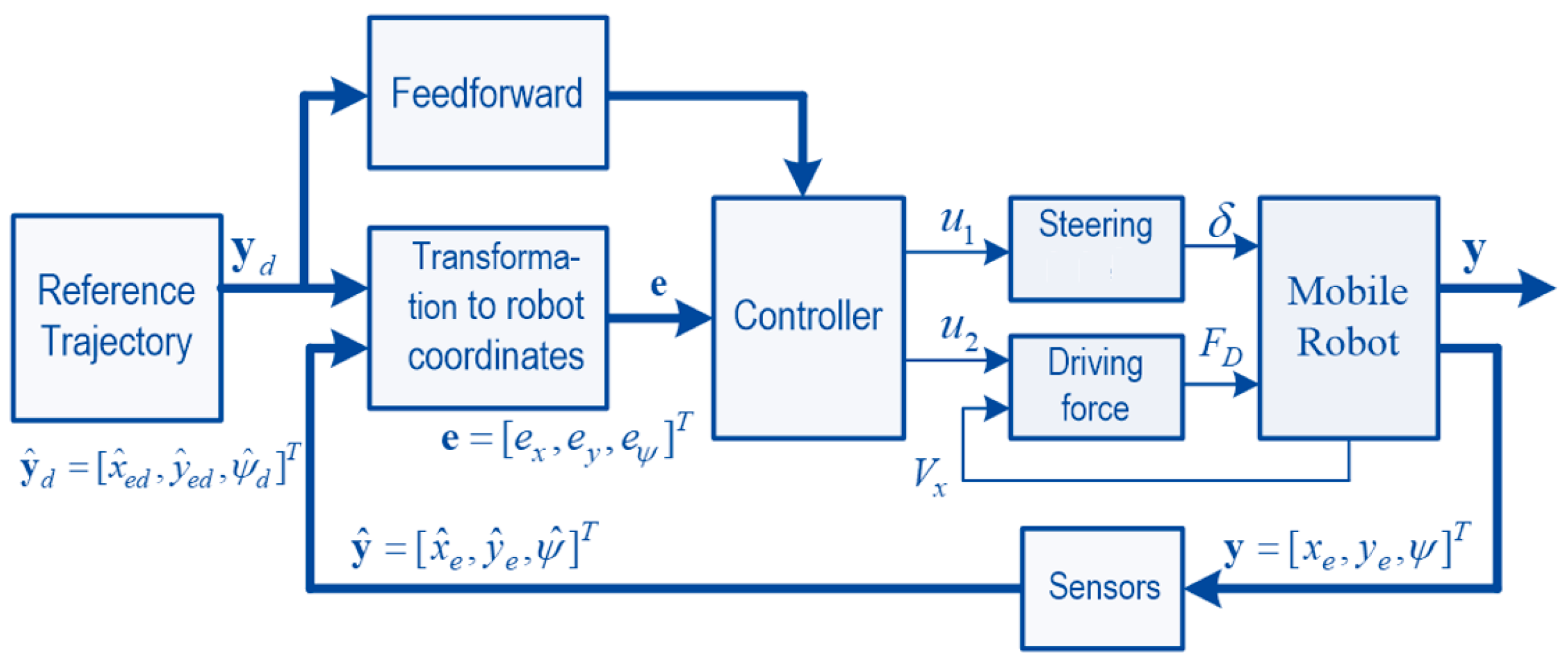
2. Materials and Methods

This study presents a control system designed for a 20 DOFs robotic platform, integrating nonlinear dynamic equations and machine learning models. The robot is modeled using a set of nonlinear differential equations, and the control system is developed using MATLAB. The dynamic modeling incorporates the Adams–Bashforth–Moulton method for solving the equations of motion, chosen for their balance between computational efficiency and accuracy in predicting dynamic states. The hybrid control strategy combines traditional feedback control and a neural network that dynamically adjusts the control parameters based on real-time sensor inputs. The neural network is trained on historical data collected from the robot’s previous trajectories, allowing it to predict necessary adjustments for improved performance in real-world tasks.

2.1. Mathematical Foundation and Dynamic Modeling

The flyer model was adapted, which is extensively detailed in the literature [23] and serves as the basis for the implemented software representing a complete humanoid mechanism. Figure 2 illustrates the basic model serving as the foundation for the software in MATLAB’s implementation. In this schematic representation of the humanoid robot, contact with the ground is facilitated by a cart with the specified dimensions. The primary segment of the mechanism is the pelvis, which is rigidly attached to the stationary cart. This modeling approach aligns with techniques used in robotic manipulator design, where, typically, a single open kinematic chain is sufficient to represent the manipulator.
In this case, however, due to the complexity of the humanoid structure, multiple kinematic chains are required, each originating from specific segments of the mechanism. Figure 2 depicts the mechanism as consisting of three kinematic chains, indicated by curved lines with arrows showing the direction of the chain extension. Chain I comprises the pelvis, torso, and head; chain II, the pelvis, torso, and right arm; and chain III, the pelvis, torso, and left arm.
Each chain is composed of segments (numbered: torso—4, head—7, right upper arm—10, right forearm—12, right hand—14, left upper arm—17, left forearm—19, left hand—21) in Figure 2. All other segments are imaginary with approximately zero dimensions, as well as negligible dynamic characteristics so as not to affect the real part of the mechanism (masses m and moments of inertia J, have values of 0). This division into kinematic chains is a functional approach for this model.
The head and torso segments are separated, introducing three additional degrees of freedom between them, replicating realistic movement. A rotational degree of freedom around the z-axis is introduced between the pelvis and torso, providing a third degree of freedom at the waist. The arm complexity is increased by adding two more degrees of freedom at the shoulders (allowing rotation around the y-axis) and incorporating triangular joints along the z-axis in both arms. The model includes hands, which can rotate relative to the forearm, achieved through a combination of rotations around the x- and y-axes. The resulting structure, thus, provides a total degree of freedom as given by N = 20i + 6.
The state of the robotic system is defined by the vector X [23,39], which includes the joint angles, angular velocities, and accelerations. The pose of a base segment in space is given by the following equation:
X = x ,   y ,   z , φ , θ ,   ψ T
The vector contains six components that describe the position and orientation in a three-dimensional space: x   y   z   represent the Cartesian coordinates of the position in space. φ   θ   ψ represent angles that are typically Euler angles, describing the orientation of the segment in space ( φ —roll rotation around x-axis; θ —pitch rotation about the y-axis; and ψ —yaw rotation about the z-axis).
φ ( r o l l ) = a t a n 2 · ω · x + y · z , 1 2 · x 2 + y 2
θ ( p i t c h ) = a s i n 2 · ω · z + x · y
ψ ( y a w ) = a t a n 2 2 · ω · z + x · y , 1 2 · y 2 + z 2
This vector describes the spatial positioning and orientation of an object (such as a robot) in terms of the translational coordinates x, y, z and rotational coordinates φ   θ   ψ . It is used for determining the location and orientation in space, suitable for tasks like navigation, positioning, and alignment in a fixed reference frame. Its purpose is to provide a general pose in 3D space, useful for external tasks and interactions, whereas a state vector that includes joint dynamics is more specialized for internal control and analysis within robotic systems and is given in Equation [5], which includes the joint angles, angular velocities, and accelerations. This would indeed be a more detailed and dynamic focused version of a state vector in robotics.
Q = X     q T = x     y     z     φ       θ     ψ     q 1       q 2       q 3         q n T
This vector typically encompasses not only the positions of the joints but also their velocities and accelerations over time, making it highly suitable for dynamic modeling and control purposes. The dynamic model, governed by nonlinear dynamic equations derived from the Euler–Lagrange formulation [40,41], for a robotic system with n degrees of freedom (DOFs) is described as follows:
H q q ¨ + h q , q ˙ + g ( q ) = τ
where
  • H q is the inertia matrix, influenced by the robot’s configuration;
  • q ¨ represents the joint accelerations;
  • h q , q ˙ represents the Coriolis and centrifugal forces, dependent on both the position and velocities of the joints;
  • g q is the gravitational force vector, depending solely on its configuration;
  • u is the control input vector (torques or forces).
The robot’s velocity motion is governed by the following differential equations:
q ˙ = c o s θ 0 s i n θ 0 0 1 v ω
where q represents the joint positions, θ represents the orientation, υ represents the linear velocities, and ω represents the angular velocities. The key engineered features include the Euler angles (derived from quaternion orientation data), total angular velocity ( ω t ) , and total linear acceleration ( v t ) .
ω t = a n g u l a r _ v e l o c i t y _ X 2 + a n g u l a r _ v e l o c i t y _ Y 2 + a n g u l a r _ v e l o c i t y _ Z 2
v t = l i n e a r _ a c c e l e r a t _ X 2 + l i n e a r _ a c c e l e r a t _ Y 2 + l i n e a r _ a c c e l e r a t i _ Z 2
Analyzing the movement of the robot in the environment, the Jacobian matrix is used, J = X Q   , which gives the relationship between the point of the robot located in the local coordinate system and the speed of the entire mechanism in relation to the global coordinate system:
H q q ¨ + h q , q ˙ + g q = τ + J T   ( q )   F e x t
J T   ( q ) is the transpose of the Jacobian matrix. This matrix relates the external forces and torques   F e x t acting on the robot to the torques at the joints. The Jacobian J(q) transforms the joint velocity vectors into end-effector velocity vectors in the workspace, and its transpose J T   q maps the external forces applied to the end-effector back to the equivalent joint torques.
  F e x t represents the external forces. This vector represents the forces and torques from the environment acting on the robot. These could be due to interaction with objects, external loads, or any other environmental influence exerting force on the robot.
In an IoT-integrated robotic system, the motion of the robot can be monitored through a connected device that communicates with the controller, publishing pose data in a structured format, such as JSON sensor data for “current_pose”, which include information about the robot’s position and orientation (the position of the robot’s tool reference frame is described by the coordinates in Equation (1) and the orientation by Equation (5)).
Once all of these data are organized, they are ready to be used to create a virtual “flyer” object. However, before using this object, it must first be created in the computer’s memory. This is performed with the help of the k_flier constructor. When this constructor is called, it creates a new flyer object (in this case, named flier20), based on the structured data from the gen_links function.
In simple terms, the ‘gen_links’ function gathers all the complex information needed to define the flyer, while the ‘k_flier’ constructor brings it to life in the digital environment, allowing researchers to use this model in simulations and to further study its behavior.
The flowchart (Figure 3) effectively outlines a robust system for managing commands in an automated or robotic system, ensuring that actions are taken based on successful connections and accurate sensor data, with contingencies for failures. It emphasizes a structured approach to operational readiness, monitoring, and execution, allowing for real-time adjustments and precise control based on environmental feedback and operational status. The integration of feedback loops and error checks promotes high reliability and safety, crucial for maintaining performance and responsiveness in dynamic environments.

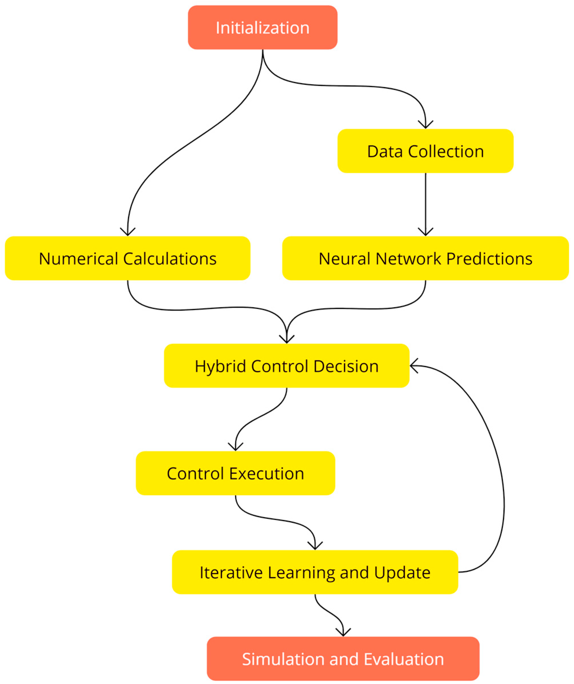
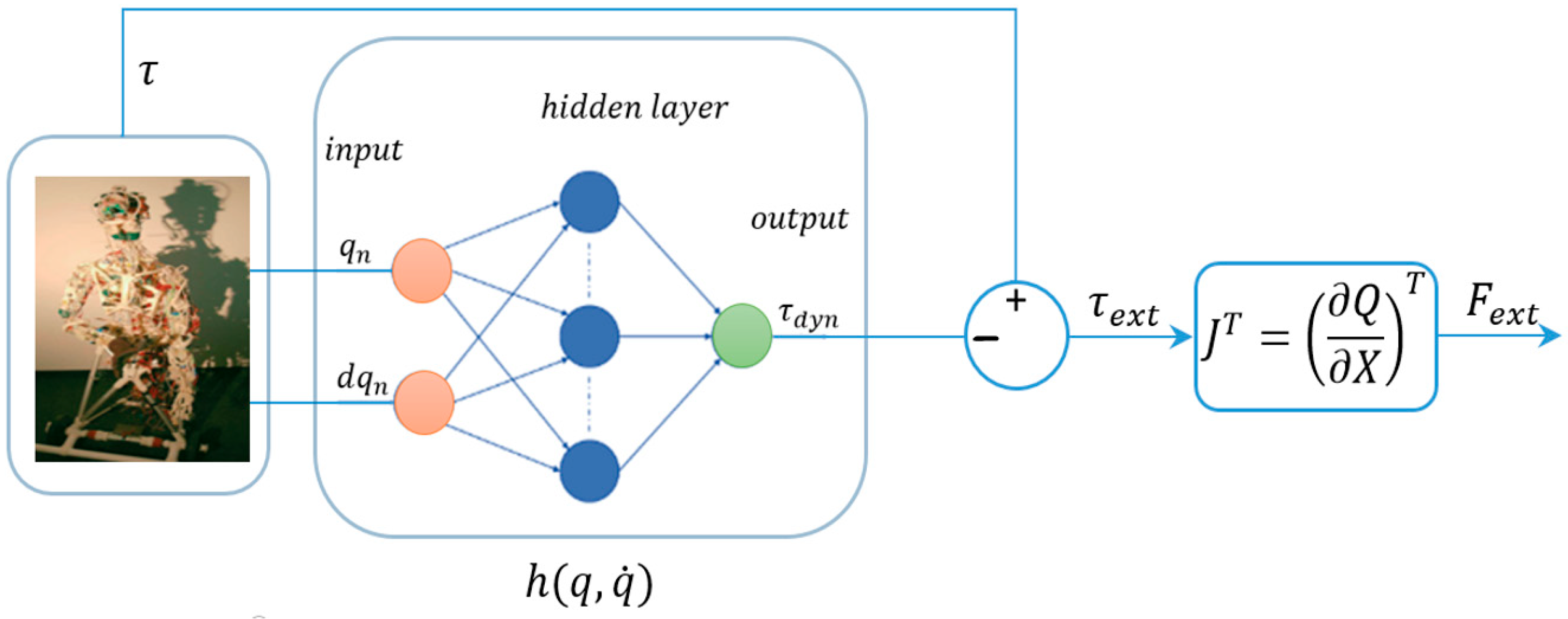
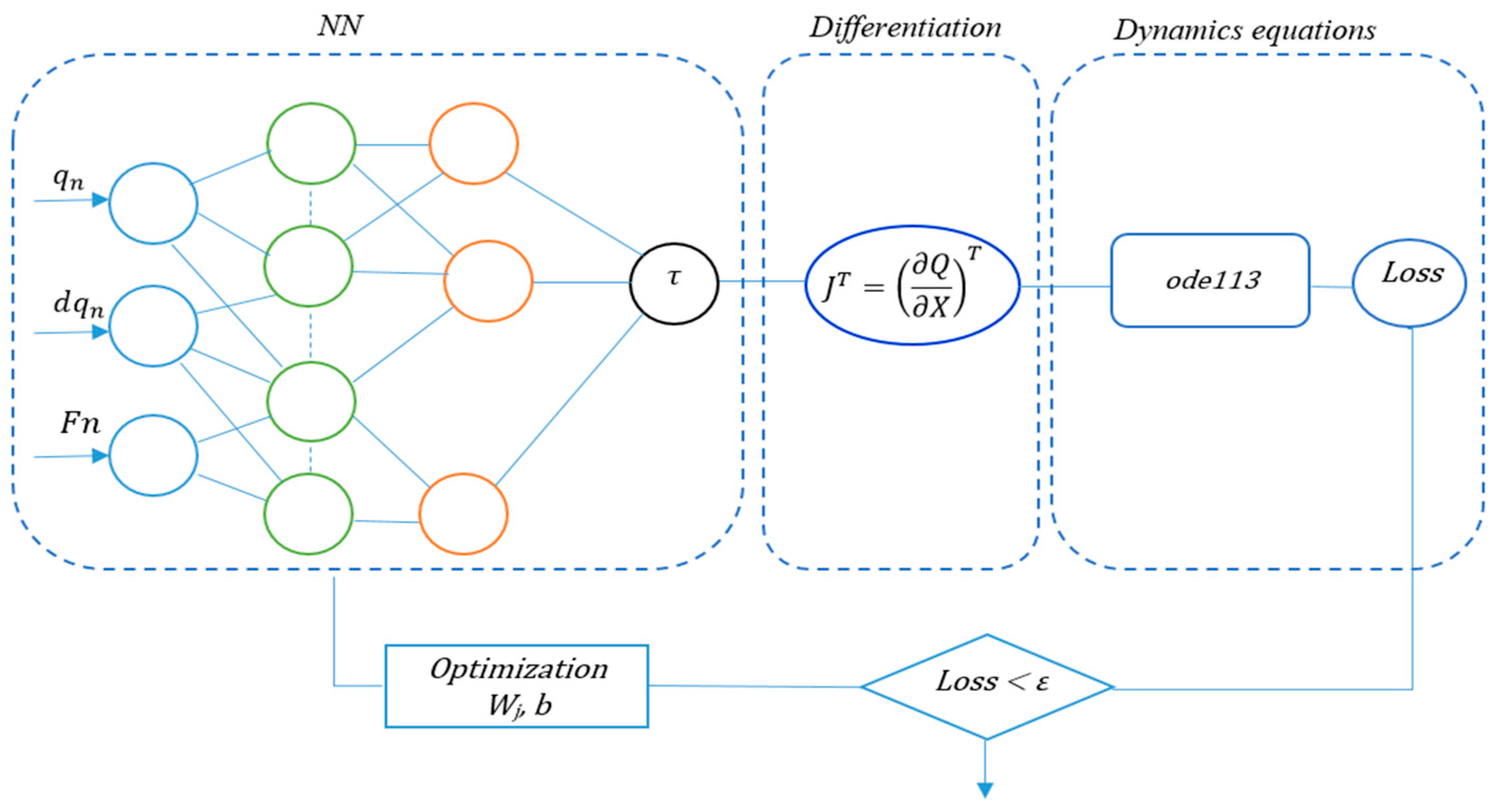
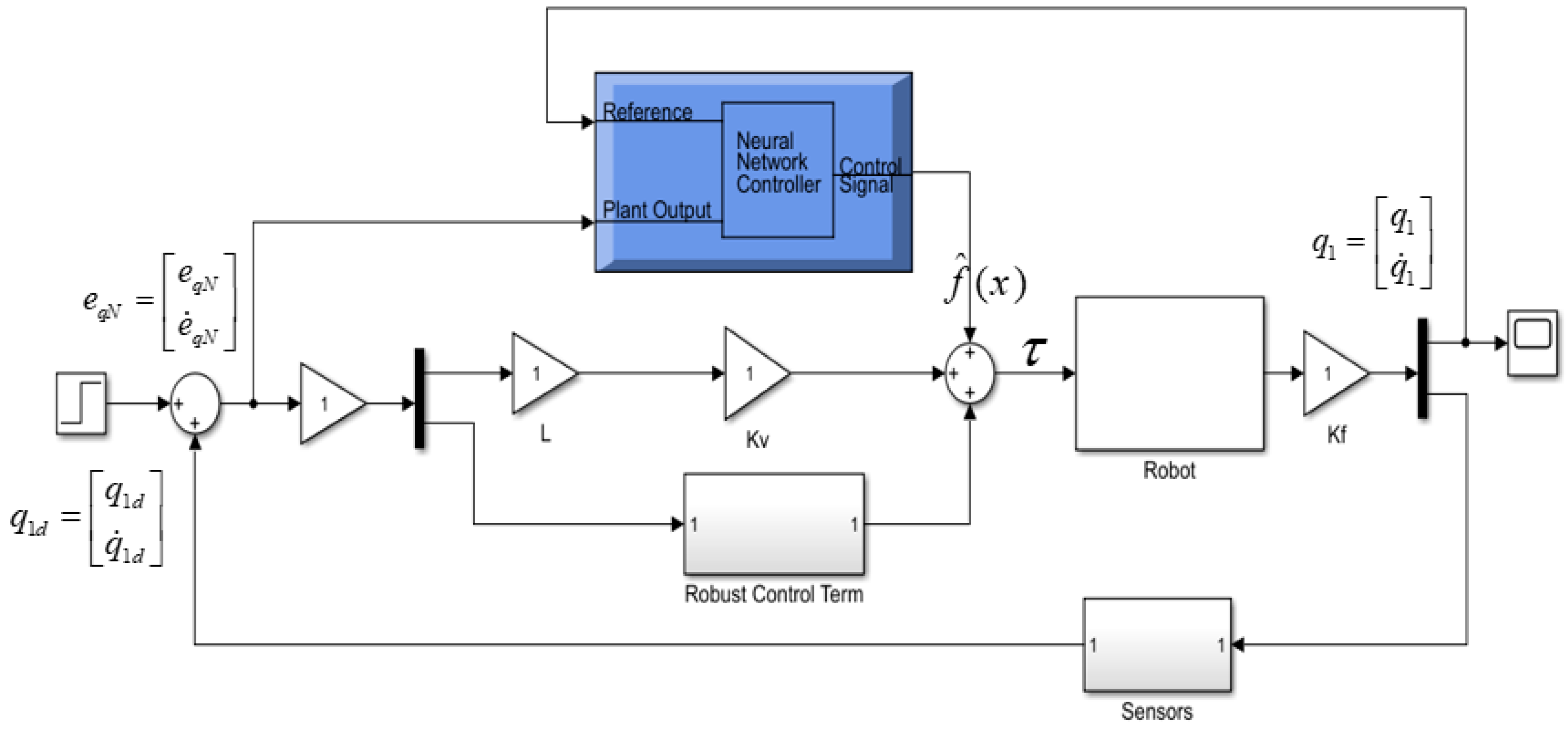
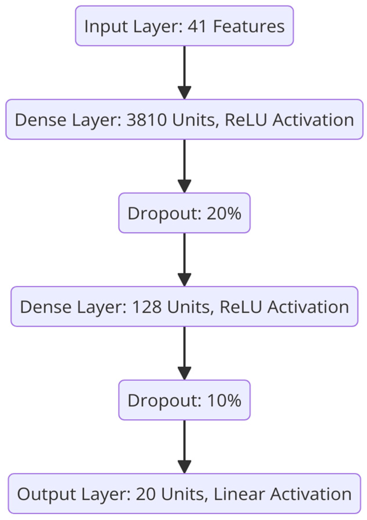
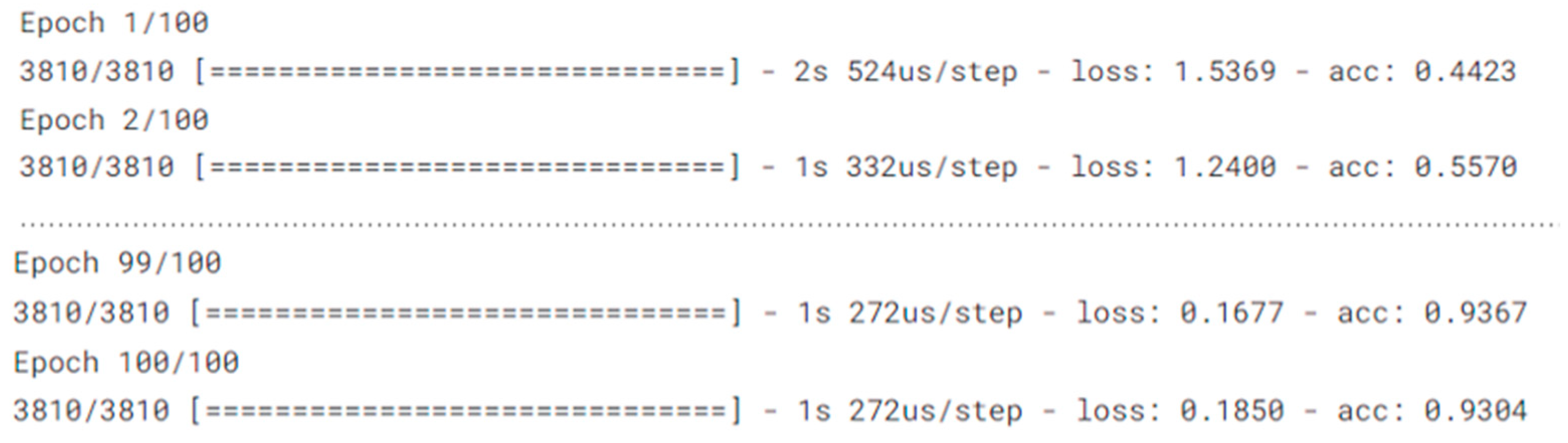
2.2. Integrating Nonlinear Methods with Neural Networks

The diagram in Figure 4 outlines a hybrid control architecture that integrates traditional numerical calculations with neural network predictions to optimize robotic control. This architecture is designed to adaptively refine control strategies through iterative learning, making it highly effective for complex robotic applications. We proposed a hybrid control architecture that combines the strengths of nonlinear mathematical methods and neural networks. A neural network is used to optimize the robot’s control strategy, such as path planning, joint control, or disturbance handling. The inputs to the neural network were as follows: the joint angles, joint velocities, external forces, etc. The outputs of the neural network were as follows: the predicted joint torques, optimized trajectories, or control signals.
Machine learning models are integrated to learn from the robot’s past trajectories and to dynamically adjust the control parameters.
The inputs to the neural network are the variables that describe the current state of the robot and the environment. In this case, these include the following: the position of each joint in the robot, which can be represented as a vector Q (Equation (5)) of size n, where n is the number of joints   q = q 1 ,   q 2 ,   ,   q n   the speed at which each joint is moving (vector d q = q ˙ ) of size n: d q = q ˙ = q ˙ 1 , q ˙ 2 , q ˙ 3 ,     q ˙ n   ; and the external forces acting on the robot (including disturbances, gravity, or forces from contact with the environment). F = F x ,   F y ,   F z   , where the components are forces in the three-dimensional space. The previous control signals or torques applied to the joints are used as inputs if the control strategy depends on past actions.
Applying Equation (5), the outputs of the neural network are the variables that represent the control actions the robot should take (Figure 5). The joint torques τ are applied to each joint to achieve the desired motion. With a vector τ of size n, y = τ 1   τ 2   τ 3     τ n T , and the desired angles q n (joint positions) and q ˙ n (joint velocities) for each joint, the robot should be guided by the neural network to a specific posture or trajectory.
From the MATLAB robot code, the inputs are as follows: q(7:26), the angles of the robot’s joints; dq(7:26), the velocities of the robot’s joints; and FW, the external forces acting on the robot.
Outputs: The torque values that should be applied to each joint to achieve that which is desired, such as from the main loop of the neural network, where the torques (currently with physics-based models) are calculated.
Neural network architecture: The input layer has a size 2n + m, where n is the number of joints, and m is the number of force components. Hidden layers: the number of layers and neurons are chosen per layer based on the complexity of the control problem. A common starting point is two hidden layers with 64 neurons each. The output layer has a size n, corresponding to the torques for each joint. Activation functions: typically, the ReLU (Rectified Linear Unit) is used for the hidden layers and a linear activation for the output layer.
The control strategy for the robotic system involves using the torques predicted by a neural network to precisely actuate the robot’s joints. This method incorporates real-time data on the joint positions, velocities, and external forces to calculate the necessary torques (Figure 6). These torques are then applied directly to the joints, enabling the robot to achieve the desired movements and postures efficiently. This approach ensures both accuracy and reduced energy consumption, enhancing the robot’s performance and durability.
Weight matrices ( W 1 ,   W 2 , ,   W j ) are used in each layer of a neural network to transform the input data into a format that the network can use to make decisions or predictions. For instance, W 1 is the weight matrix used in the first layer of the network to transform the initial input vector into the first hidden layer’s output (h1). Similarly,   W 2 transforms h1 into h2, and so on. Neural networks use weight matrices in conjunction with nonlinear activation functions (like the ReLU) to introduce nonlinearity into the network. This nonlinearity allows the network to learn complex patterns beyond what a linear model could achieve.
During the training phase, these weight matrices are adjusted to minimize the loss function—the measure of how far the network’s predictions are from the actual values. This is typically performed using optimization algorithms like gradient descent, where W j is updated iteratively. This is described by the following equation:
W j ( t + 1 ) = W j ( t ) μ L W j
W j denotes the weight matrix at the j-th layer at iteration t. The gradient L W j tells us how to adjust W j to reduce errors in the predictions, and η is the learning rate that determines how big each update should be.
W 1 and W j are crucial for transforming and processing the input data through each layer of the network, allowing the model to learn from the data and make increasingly accurate predictions or control decisions. The use of multiple weight matrices enables the network to handle a variety of tasks and adapt to different data patterns and complexities, which is especially vital in applications like robotic control where the dynamics can be highly variable and complex.
The main loop of the MATLAB code (Algorithm 1) performs the execution of the planned motions:
Algorithm 1 Predict Function
 1:
while (t < T)
 2:
  t = i*dt;
 3:
  % Update the states
 4:
  Q_132 = [q; TetaA; TetaB; dq; dTetaA; dTetaB];
 5:
  options = odeset(‘RelTol’, 1 × 10⁻², ‘AbsTol’, 1 × 10⁻⁴, ‘MaxOrder’, 3);
 6:
  [tout,Q_132_out] = ode113(@ECCERdof_PomPod,[t t + dt], Q_132, options);
 7:
  Q_132 = Q_132_out(end,:)’;
 8:
  q = Q_132(1:26);
 9:
  …
10:
  % Control adjustments
Here, the robot states (positions, velocities, etc.) are updated over time using a numerical integration method (ode113), which approximates the continuous time dynamics of the robot.
The loss function is defined as the mean squared error between the desired and actual joint angles. The training process involves backpropagation, where the gradients of the loss function are computed with respect to the network parameters and used to update the weights.
Loss function. The mean squared error (MSE) between the predicted torques y ^ and the actual torques y is determined as follows:
Ը = 1 n i = 1 n y ^ i y i 2

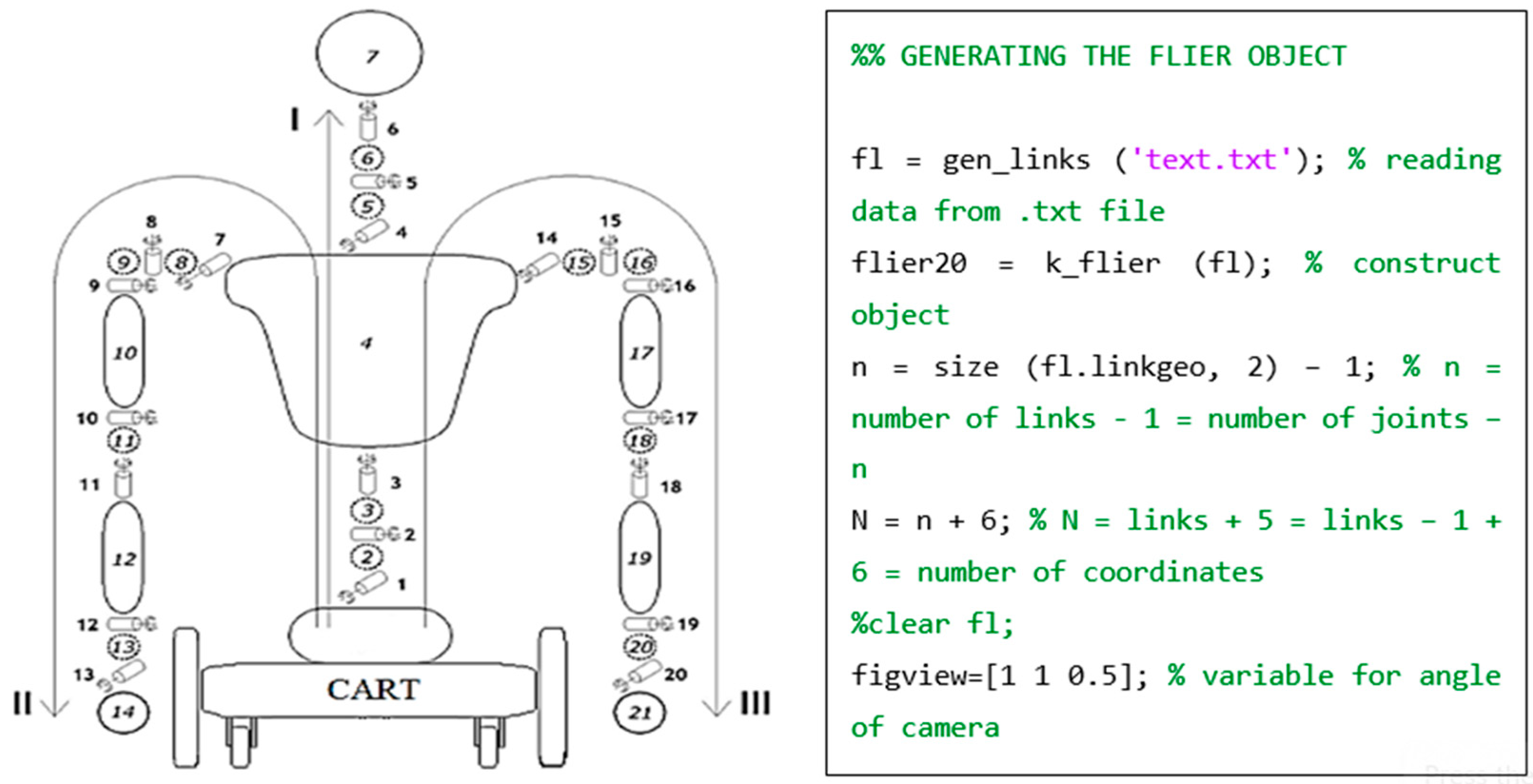
2.3. Adams–Bashforth–Moulton Method for Nonlinear Dynamics

The dynamics of the 20 DOFs robot are simulated using the ode113 solver, which implements the Adams–Bashforth–Moulton method. This method is particularly well suited for solving stiff ordinary differential equations (ODEs), which are common in robotic systems due to the presence of multiple interacting components. The Adams–Bashforth–Moulton method is a predictor–corrector method used to solve ODEs of the form y ˙ = f ( t , y ) .
The predictor step estimates the solution at the next time step using the previous values:
y n + 1 p r e d i c t = y n + h i = 0 m 1 β f ( t n 1 , y n 1 )
The corrector step refines the estimate to enhance the accuracy:
y n + 1 = y n + h 2 0 f ( t n + 1 , y n + 1 p r e d i c t ) + i = 0 m 1 i f ( t n 1 , y n 1 )
where h is the step size and βi and αi are the coefficients that depend on the order of the method.
This method is particularly effective for ensuring that the solution remains stable and accurate over long simulation periods, making it ideal for scenarios that integrate both the outputs from numerical methods and adjustments from machine learning to generate the optimal control inputs for the robotic system.
The hybrid control strategy, combining traditional control (PID and inverse kinematics) with machine learning for model-free adaptation, can be implemented within the controller block. The transformation to robot coordinates and feedforward components would be primarily handled by traditional control methods, while the controller can adapt using machine learning to fine-tune responses based on sensor feedback.
The provided diagram (Figure 7) is consistent with the mathematical and control methodologies discussed in this paper. It effectively visualizes the hybrid control architecture where traditional control principles, numerical methods, and machine learning work together to optimize the robotic motion control.
The control structure can be broken down into the following stages:
Reference trajectory generator: This block generates the desired reference trajectory defined by x e d , which is the desired position in the x-direction; y e d , which is the desired position in the y-direction; ψ e d , which is the desired heading angle; and V d , which is the desired velocity.
The feedforward block compensates for known disturbances and path deviations. In the methodology discussed earlier, this is supported by the traditional control methods, where the feedforward signal works as a primary reference, while the feedback corrects errors.
Coordinate transformation and guidance errors: This block transforms the global reference trajectory into the robot’s local coordinate frame. It computes the errors between the desired trajectory (from the reference generator) and the current trajectory of the robot.
The outputs include the following: e ψ , which is the error in the heading angle and e x ,     e y , which are the position errors in the x- and y-directions. The desired heading and velocity values ψ e d ,   V d are passed to the controller.
The controller processes the errors and generates control signals u 1 and u 2 , which correspond to the commands for the steering wheel and driving force, respectively. The controller seeks to minimize the errors e ψ and e x ,   e y by adjusting the steering and speed commands.
This is analogous to the inverse kinematics calculation q = f 1 ( p ) .
Controller: The controller block is responsible for generating the actuation commands u 1 (steering) and u 2 (driving force). In the context of the earlier methodology, this would involve both traditional control (PID and adaptive control) and machine learning components for fine-tuning the actuation.
The mathematical formulation for control is presented with the following equations:
u 1 = K p e x + K i e x d x + K d d e x d t
u 2 = K p e ψ + K i e ψ d x + K d d e ψ d t
where K p ,   K i ,   K d are the control gains, adaptively tuned using the neural network; ψ d is the desired heading angle; and   ψ is the current heading angle.
Mobile robot dynamics: The dynamics of the mobile robot, such as the steering and driving forces, are controlled by the inputs u 1   and u 2 . This block represents the physical model of the robot, whose dynamics were mathematically modeled using the Adams–Bashforth–Moulton method.
Sensors and feedback loop: The sensor block provides the actual state y = x e ,   y e ,   ψ T back to the controller for feedback-based correction. The sensor inputs, such as the current pose (position and orientation), are used to refine the predictions from the neural network and the Adams–Bashforth–Moulton method, ensuring precise real-time feedback and minimizing the error e ( t ) .
Results and feedback loop: The outputs of the mobile robot block (current positions x e , y e ; heading   ψ ; and velocity V x ) are compared to the desired reference values x e d ,     y e d ,     ψ ,   V d to continuously adjust the control inputs. The feedback loop ensures that the robot stays on the desired trajectory by constantly minimizing the errors through corrective actions from the controller.
The key equations that are applied in this architecture involve computing the trajectory errors, updating the control laws, and modeling the robot’s motion [42], based on its dynamics (typically represented by differential equations).
The diagram represents a closed-loop control system for trajectory tracking, where the robot continuously receives updated trajectory information and makes real-time adjustments to its steering and speed to follow the reference path. The control system integrates sensor feedback and guidance algorithms to ensure accurate path following.
Forward kinematics is the process of determining the position and orientation of the end-effector (in task space p) from the joint angles (in configuration space q).
Mathematically, it is represented as follows:
p = f q
where
  • p is the position and orientation of the end-effector in the task space;
  • q is the vector of the joint angles in the configuration space;
  • f is the forward kinematics function.
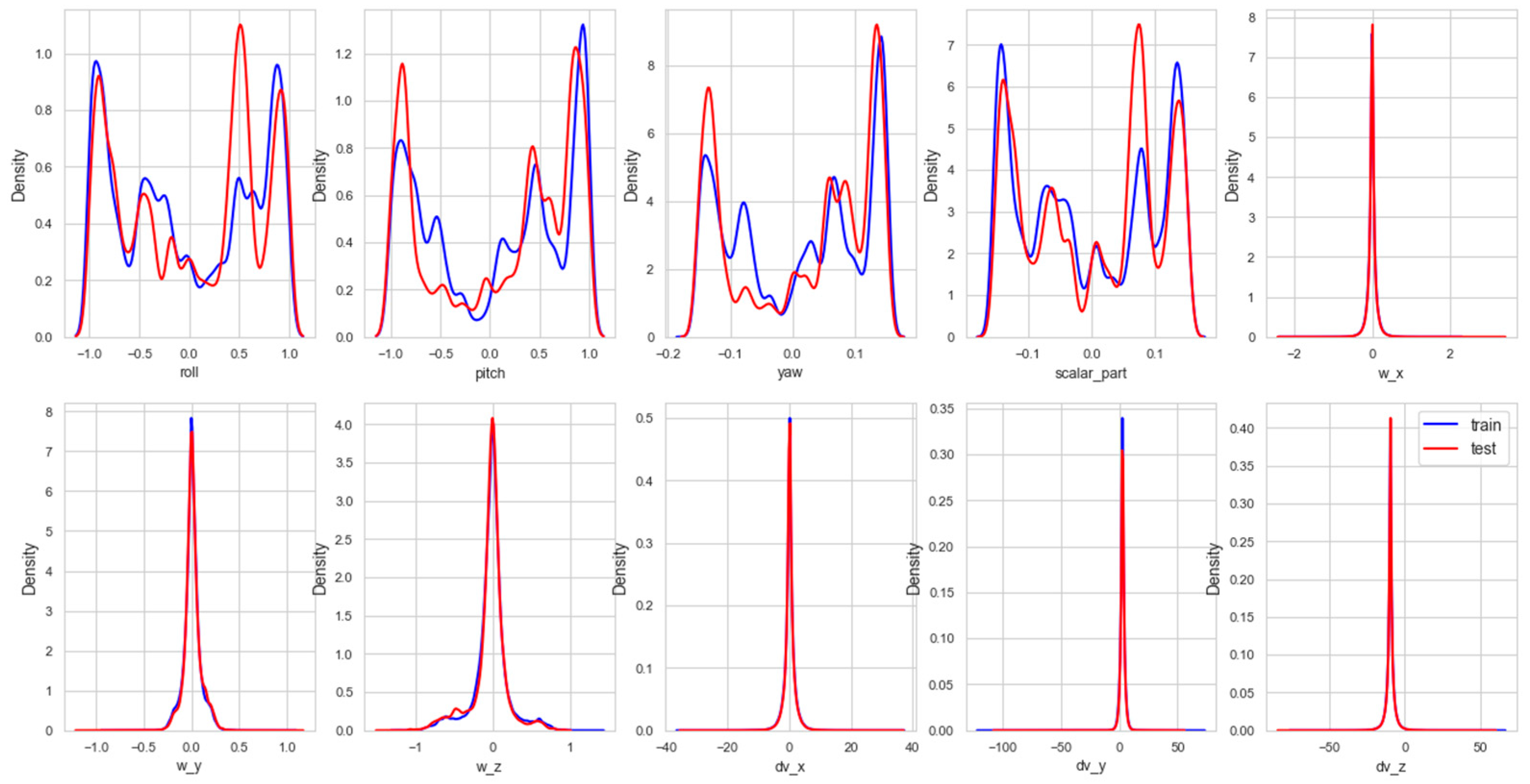
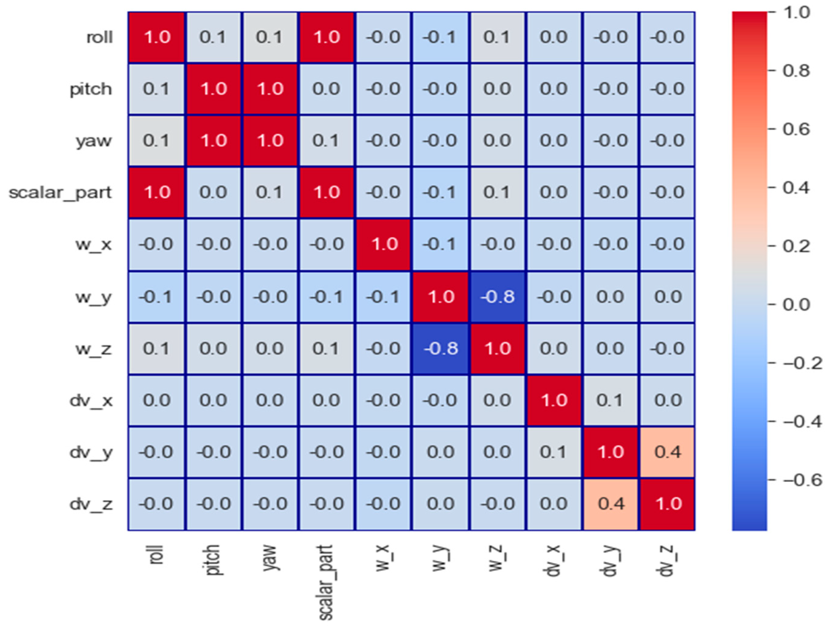
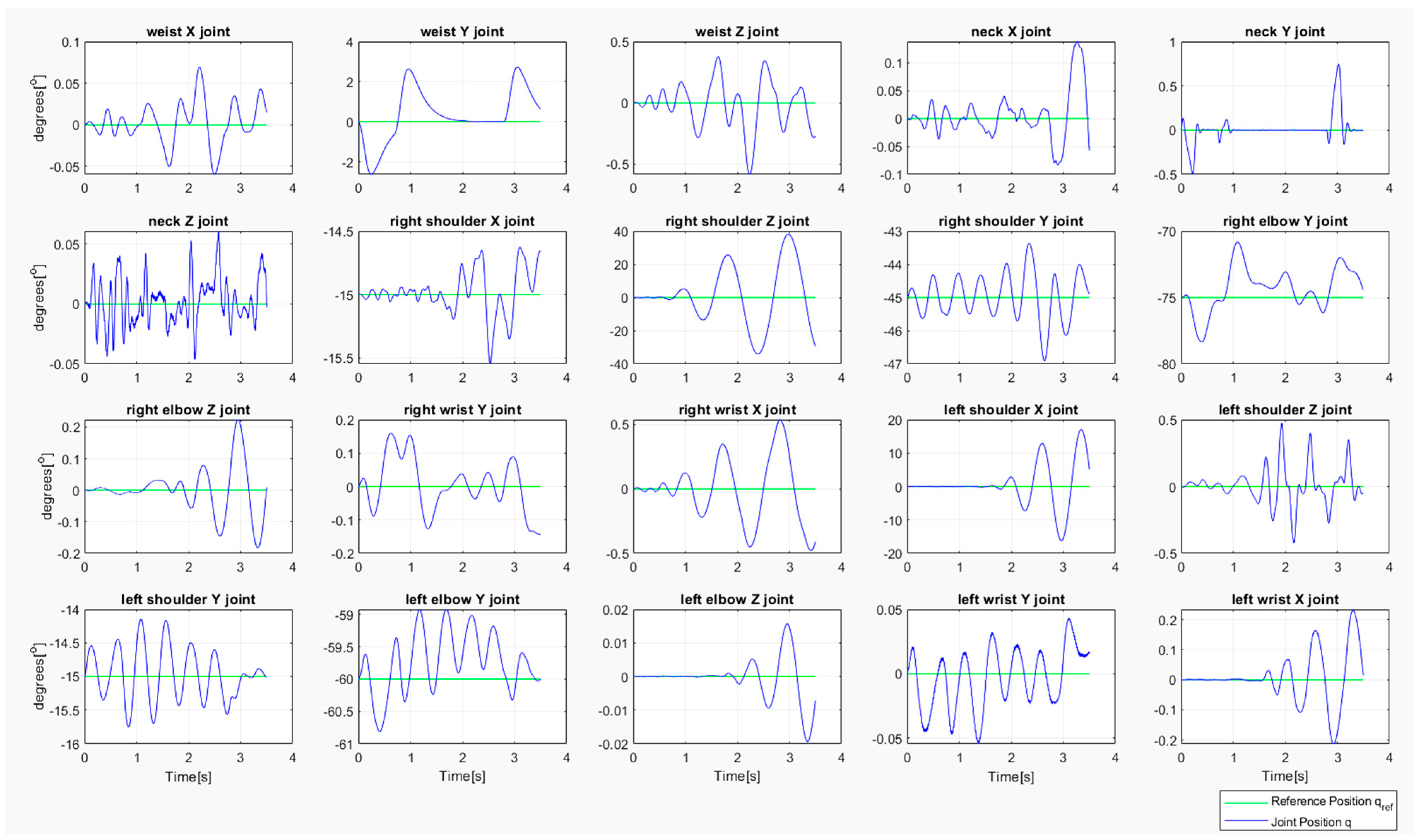
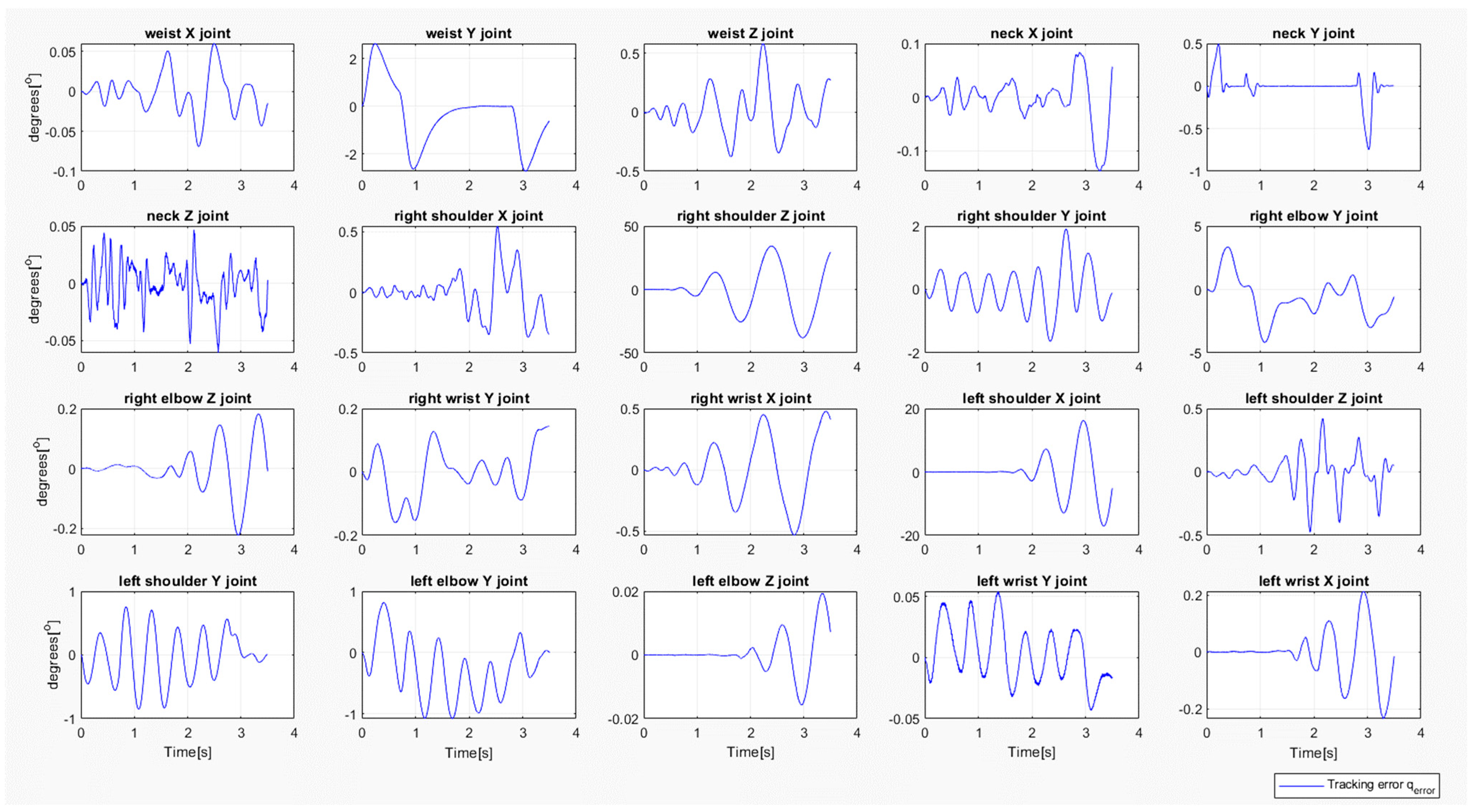
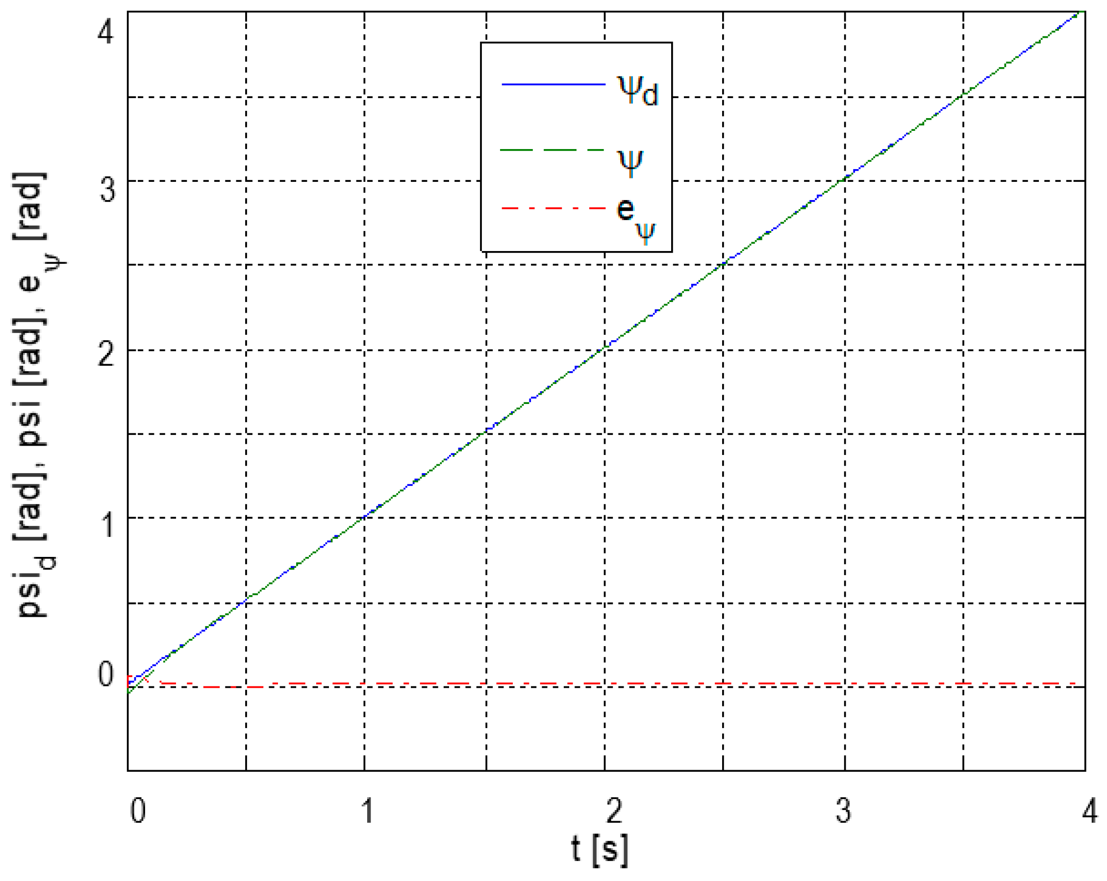
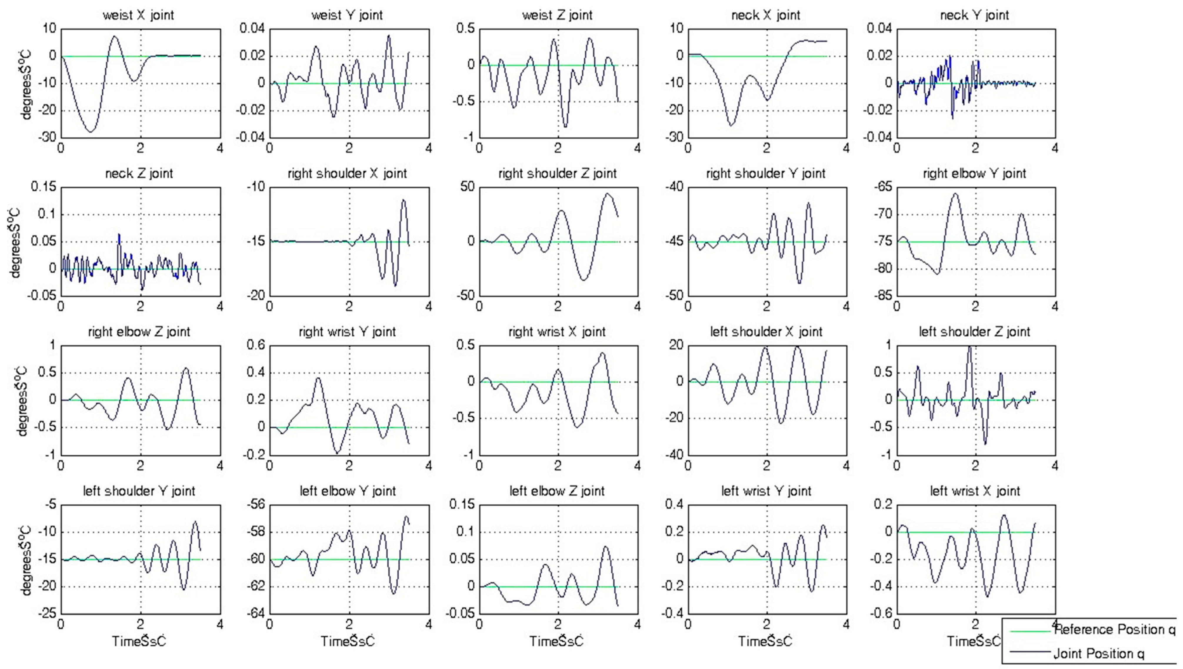
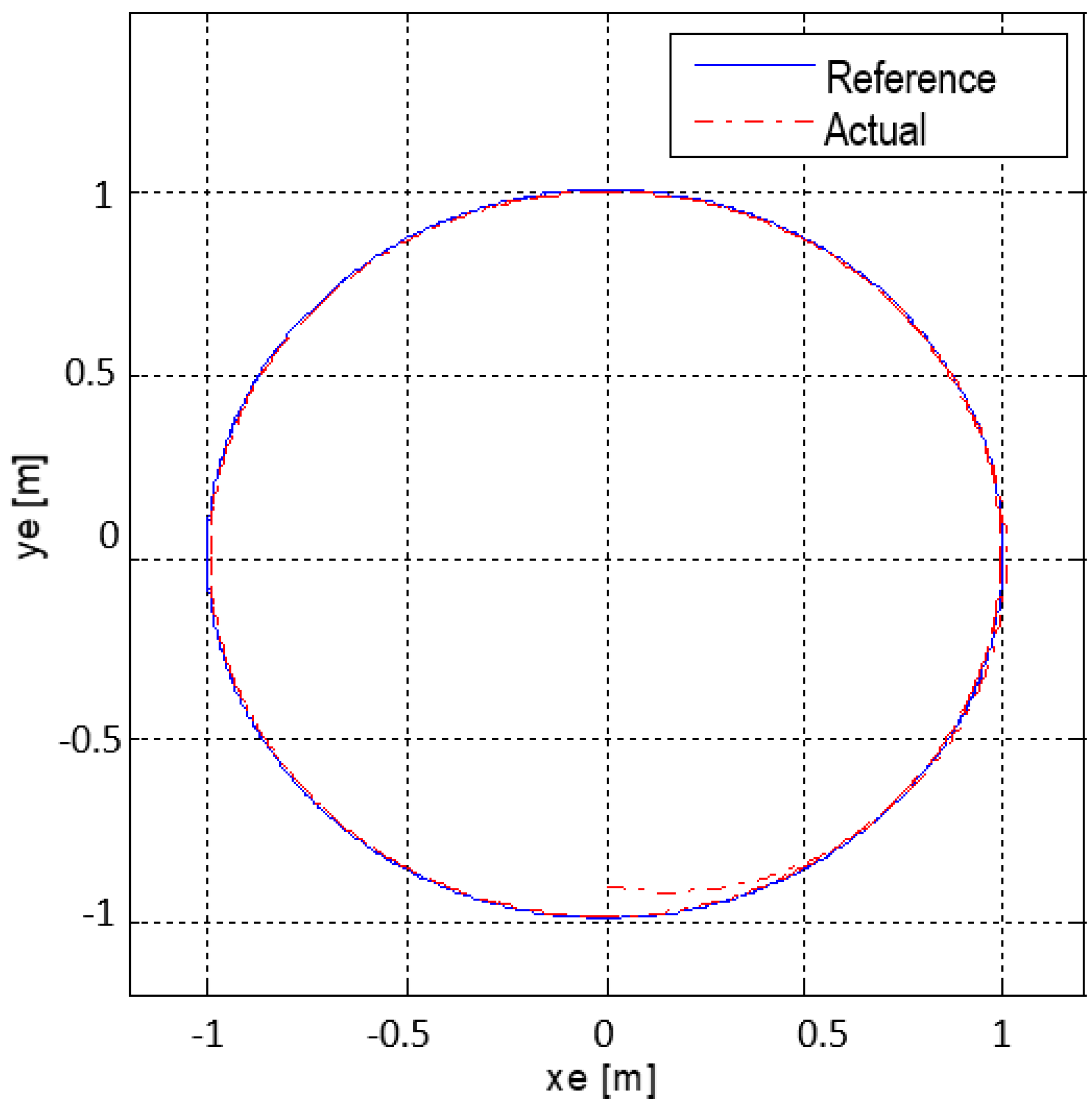
This function maps the joint angles to the end-effector’s position and orientation in the task space.
Inverse kinematics is the process of determining the required joint angles (in configuration space q) to achieve a desired position and orientation of the end-effector (in task space p).
Mathematically, it is represented as follows:
p = f 1 q
where q is the vector of the joint angles in the configuration space; p is the desired position and orientation of the end-effector in the task space; and f−1 is the inverse kinematics function. This function maps a desired end-effector position and orientation back to the necessary joint angles.
Mapping the relationship between the spaces: the actuation inputs u are mapped to the configuration space q using specific functions, denoted as f s p e c 1 .
From configuration space to task space: the joint angles q are then mapped to the task space p using the forward kinematics function:
  p = f f i n d q
Inverse mapping: conversely, the task space p can be mapped back to the configuration space q using inverse kinematics, f f i n d 1 , and then from the configuration space to the actuation space using f s p e c .
q = f f i n d 1 p
u = f s p e c q
Forward process: u (actuation) →   q (configuration) →   p (task space).
Inverse process: p (task space) →   q (configuration) →   u (actuation).
The forward kinematics f maps the joint angles to the task space positions, while the inverse kinematics f 1 maps the task space positions to the necessary joint angles. The additional mappings f s p e c and f s p e c 1 connect the actuation commands with the configuration space, effectively linking the entire control system from the actuator inputs to the task-specific outputs.
The system’s foundation is built on mathematical equations representing inverse kinematics and the dynamic model of the robot. The equations below define the positional errors and control inputs: e x = x d x   e y = y d y   e ψ = ψ d ψ .
The robot’s control inputs u 1 and u 2 are derived based on these error measurements and are fed into the controller to generate the desired driving force FD and steering wheel commands δ.
In Figure 8, the control system, which integrates both the traditional control methods and a neural network within a hybrid control architecture, is presented. This configuration is composed of two main loops: the tracking loop and the nonlinear inner loop with a neural network.
The tracking loop generates the desired trajectory signals, including the reference positions q 1 d and velocities q ˙ 1 d , and computes the trajectory errors e and e ˙ . These errors are processed through the gain matrices L and K v to produce a reference signal that guides the robust control term and the nonlinear inner loop. The summation operation, represented by the plus sign in the diagram (Figure 8), combines the reference signals and feedback states to compute the error signals. By minimizing these errors, the tracking loop ensures that the robot’s movement remains as close as possible to the desired path.
The nonlinear inner loop incorporates a neural network that provides an adaptive control term f ^ ( x ) . This neural network estimates and compensates for the nonlinearities and uncertainties in the robot’s dynamics, particularly those not addressed by the traditional control elements. The neural network receives inputs corresponding to the robot’s states, including positions and velocities, and outputs an adaptive control signal f ^ ( x ) . This signal is combined with the robust control term v ( t ) , enhancing the system’s adaptability and providing improved tracking accuracy by adjusting to dynamic changes in real time.
The robust control term v ( t ) provides stability to the control system by handling model uncertainties and disturbances. It receives the reference input τ from the tracking loop and works in conjunction with the adaptive term f ^ ( x ) generated by the neural network. Unity gain, represented by the number “1” in the diagram, indicates that certain control signals pass through unchanged as they proceed to different stages of the system. The robust control term, therefore, adds an additional layer of reliability, ensuring that the system remains resilient to unexpected changes and modeling inaccuracies.
The robot system block represents the actual physical dynamics of the robot. The combined output from the robust control term and force control loop is fed into this block, which calculates the resulting joint positions q 1 and velocities q ˙ 1 . The feedback from these actual states is looped back into the tracking and force control loops, allowing the control system to continuously refine its actions based on the current robot state, ensuring accurate trajectory tracking and force application.
Unlike conventional feedback mechanisms, which typically rely on fixed control gains or linear models, the neural network adapts in real time based on state feedback, providing an output f ^ ( x ) that is combined with the robust control term v ( t ) . The combined control input to the robot system is τ = v t + f ^ ( x ) . The error e in the tracking loop e = q d q . By leveraging the neural network’s learning capabilities, the control law becomes adaptive, ensuring that the system can cope with dynamic environmental changes, which is especially valuable in applications involving variable loads or complex trajectories. The prediction error e q N = F ( x ) f ^ ( x ) is associated with the neural network’s approximation defined as follows. If we make a comparison to traditional control, in this neural network control model, L functions similarly to K p (proportional control). Kf is a gain matrix that determines how the system reacts to differences between the desired and measured interaction forces. K v plays a role akin to K d (derivative control), and the effect of K i (integral control) is adaptively handled by the neural network’s feedback learning capability and the robust control adjustments over time.

3. Results

An examination of the feature distributions between the training and test datasets is presented in Figure 9 and Figure 10.
Figure 8 displays the basic sensory data acquired from the robot, including orientation, angular velocity, and linear acceleration along different axes. The distributions reveal consistent patterns between the training and test data, indicating that the experimental setup effectively captures the dynamic behavior of the robotic system under varied conditions.
Figure 9 further extends this analysis to include engineered features that are critical for the robotic control algorithms, such as the total angular velocity and Euler angles.
This plot showcases the distributions for the engineered features such as the total angular velocity, total linear acceleration, Euler angles, and derived velocity and acceleration metrics in the training and test datasets.
The consistency across these feature distributions validates the data processing and feature engineering steps undertaken, ensuring that the machine learning models trained on these data are well equipped to generalize from training to real-world application scenarios. This robust feature engineering is further supported by the correlation analysis presented in Figure 11, which provides a deeper insight into the relationships between the orientation, angular velocity, and linear acceleration parameters.
From the results, as can be seen, a very strong correlation (1.0) is evident between roll (orientation_x) and scalar_part, as well as between yaw (orientation_z) and pitch (orientation_y). There is a notable negative correlation (−0.8) between angular velocity in the z-direction (w_z) and angular velocity in the y-direction (w_y). Furthermore, a moderate positive correlation (0.4) exists between linear acceleration in the y-direction (dv_y) and linear acceleration in the z-direction (dv_z). The strong correlations observed in the data not only highlight the critical relationships between the orientation and velocity parameters but also provide valuable insights into the feature importance for the subsequent predictive modeling.
In Figure 12, is presented the structure of the neural network model. The developed model consists of a sequential architecture designed to predict the robotic joint torques, which is crucial for the accurate control of a 20 DOFs robotic platform. The input layer receives 41 features, comprising the joint angles, velocities, and force measures, reflecting the comprehensive state of the robot necessary for effective torque computation.
First layer: The model begins with a dense layer of 3810 units. Although this number appears large, it was initially chosen to test the capacity of the network to capture complex patterns in the high-dimensional data. This layer uses ReLU activation to introduce nonlinearity, allowing the model to learn more complex functions.
Dropout and regularization: A dropout rate of 20% follows to prevent overfitting by randomly omitting subsets of features during training, thus ensuring that the model does not rely too heavily on any single neuron.
Hidden layers: A subsequent dense layer with 128 units further processes the learned representations, with another dropout layer at 10% to continue regularization. ReLU activation is used here as well to maintain nonlinear learning.
Output layer: The final layer consists of 20 units corresponding to each joint torque, with a linear activation function. This setup is crucial as the task is a regression problem where each output unit predicts a continuous value representing the torque.
The training progress of a neural network model is presented in Figure 13, which shows the performance over 100 epochs. It includes the loss and accuracy metrics for each epoch, demonstrating how the model’s performance improves as training progresses. As the epochs increase, the loss decreases and the accuracy increases, indicating effective learning and adaptation by the model to the training data. By the final epochs, the model achieves a high accuracy and low loss, suggesting that it has effectively captured the underlying patterns in the training dataset. The final accuracy is 0.9304 and the loss is 0.1850.

4. Simulations

Two typical cart movements, linear and circular, were simulated: a cart motion with a trapezoidal velocity profile and a circular motion.
A simulation of the robot’s cart motion with a trapezoidal velocity profile was conducted to analyze its dynamic behavior. The characteristics of the motion are summarized in Table 1.
Figure 14 presents the positions of the robot’s joints during the simulation of a cart motion with a trapezoidal velocity profile with a distance of 1 m and a time period of T = 3.5 s.
Figure 15 shows the tracking errors (tracking errors) affecting the stability during the cart motion with a trapezoidal velocity profile with a distance of 1 m, T = 3.5 s. The tracking errors indicate that the most significant deviation occurs in the X joint during the stride, but it still remains within the bounds of stability.
This research emphasizes the importance of simulations that compare the intended (reference) and actual paths that a robot follows during circular motion. By examining both the trajectory and the orientation angles (ψd for reference and ψ for actual), this study assesses how closely the robot adheres to its planned course. The tracking error (eψ), which quantifies the deviation between the robot’s actual path and its intended trajectory, as shown in Figure 16, is a critical measure in this analysis of the robot’s cart motion with a trapezoidal velocity profile.
A simulation of the robot’s circular motion was conducted to analyze its dynamic behavior. The characteristics of the circular motion, with a radius (amplitude) of 1 m and a period of 3.5 s, are summarized in Table 2.
Figure 17 presents the positions of the robot’s joints during the simulation of circular motion with a radius of 1 m and a time period of T = 3.5 s. Figure 18 shows the tracking errors (tracking errors) affecting the stability during the circular motion with a radius of 1 m and T = 3.5 s. The tracking errors indicate that the most significant deviation occurs in the X joint during the stride, but it still remains within the bounds of stability.
By examining both the trajectory and the orientation angles (ψd for the reference and ψ for the actual trajectories), this study assesses how closely the robot adheres to its planned course (Figure 19). The tracking error (eψ), which quantifies the deviation between the robot’s actual path and its intended trajectory, is a critical measure in this analysis of the robot’s circular movement.

5. Discussion

The results of this study demonstrate the efficacy of integrating nonlinear dynamics with machine learning (ML) in optimizing control systems for a 20 degrees of freedom (DOFs) robotic platform. By utilizing a hybrid control approach that combines traditional feedback methods with neural networks, the proposed system adapts to real-time changes in complex environments, such as those characterized by nonlinearity and time variance. This significantly enhances the accuracy and robustness of the robot’s trajectory tracking capabilities, particularly in IoT-driven scenarios where unpredictable disturbances and diverse environmental inputs are common.
In comparison to previous studies, this work advances the field of robotic control in several ways [43]. For instance, El-Hussieny et al. [11,44] successfully applied a deep learning-based Model Predictive Control (MPC) framework to a three DOFs biped robot leg, showing improvements in trajectory tracking. However, their focus was on a lower dimensional system and did not account for as much real-time adaptability in nonlinear environments. Similarly, Yuan et al. [24,45,46] applied auxiliary physics-informed neural networks to solve nonlinear integral differential equations, showing promise in adapting to complex environments, but with limited integration in real-time control systems for robotics.
Chen and Wen [32] explored the use of multi-layer neural networks in trajectory tracking for industrial robots. Their results highlighted the potential for ML in improving control precision, yet their study did not integrate the additional complexity of nonlinear dynamics. Our hybrid control architecture addresses this gap by providing a more comprehensive solution that allows for faster and more accurate adjustments in dynamic environments, particularly with the inclusion of real-time sensor data from IoT platforms.
This study also builds upon earlier works on robotic control using deep reinforcement learning [47,48], where Tang et al. reviewed real-world successes in the application of these techniques. While deep reinforcement learning offers significant benefits for robotic systems, our hybrid approach enhances the control system by combining machine learning models with traditional nonlinear control techniques. This hybrid method provides superior adaptability in real-time applications, particularly in IoT-driven settings.
Furthermore, Levine [49] explored deep and recurrent neural architectures for control tasks in high-dimensional robotic systems. Similarly, studies by Li et al. [33] and Zheng et al. [34] applied recurrent neural networks (RNNs) in trajectory tracking for high-dimensional robotic systems, underscoring the importance of adaptive learning models in nonlinear environments. While these works contributed valuable insights into ML applications with high-dimensional control, our study goes further by leveraging the iterative learning capabilities of neural networks within a feedback control loop, allowing for continuous system optimization in real-time scenarios.
Additionally, Wei and Zhu [50] demonstrated the application of MPC for trajectory tracking and control [51,52] in mobile robots, addressing challenges in time-varying environments. Our approach builds upon these findings by integrating neural networks to predict joint torques directly, allowing for faster adaptation and reduced computational complexity in real-time robotic control.
Moreover, the integration of the IoT with robotic control systems has been extensively discussed, particularly in smart farming applications where real-time data processing and adaptability are crucial [35,36,37]. This study further advances the field by demonstrating how an IoT framework can enhance the efficacy of ML models in dynamically adjusting the control parameters based on real-time sensor inputs [44]. The adaptability of this system is critical for environments requiring constant adjustments due to rapidly changing conditions [42].
Our neural network model demonstrated a high accuracy and low loss, with a final accuracy of 0.9304 and a loss of 0.1850. These results suggest that the model effectively captured the underlying patterns in the training dataset, demonstrating strong potential for real-world application in robotic control systems. However, while this level of accuracy is commendable, there is room for improvement when compared to the results obtained in studies such as that of Almassri et al. [53], where a neural network approach integrated with Inertial Measurement Unit (IMU) and Ultra-Wideband (UWB) data fusion achieved a 99% positioning accuracy for moving robots.
The combination of nonlinear control methods, machine learning, and IoT technologies creates a robust platform for future research and development. While this study provides a solid foundation, there are several avenues for future work. One area of focus could be improving the scalability of the system for even higher degrees of freedom in robotic platforms. Additionally, exploring more advanced neural network architectures, such as deep reinforcement learning models, could further enhance the system’s adaptability and decision-making capabilities in highly uncertain environments.
Moreover, future studies could investigate the integration of other emerging technologies, such as edge computing and 5G, to further reduce latency and improve real-time control in IoT environments [54,55]. The potential to extend this hybrid approach to other industries, such as autonomous transportation or healthcare robotics, offers promising directions for further exploration [56,57].
Among these factors, model inaccuracies and sensor delays contribute most significantly to the total tracking error. Neural network prediction errors are also influential, but their impact can be minimized with adequate training. Understanding these contributions allows for targeted improvements in model accuracy, network training, and delay management strategies to enhance real-world performance. In an IoT environment, where communication delays can occasionally occur, the control system’s inherent robustness—derived from the combination of the robust control term and the adaptive neural network—enables it to tolerate short-term data unavailability or latency. If the delays are persistent, further techniques such as predictive control can be integrated into the system, where the neural network could predict the likely future states based on historical data, thus maintaining continuity in the control response.

6. Conclusions

The integration of nonlinear dynamics, machine learning, and the IoT in this study demonstrates significant improvements in robotic control system performance, particularly in real-time adaptability and precision. These findings contribute to the growing body of knowledge in intelligent control systems and present valuable insights for future developments in both industrial and research applications.

Author Contributions

Conceptualization, V.A.K., O.P. and J.G.K.; methodology, V.A.K.; software, V.A.K.; validation, V.A.K.; formal analysis, V.A.K., O.P. and J.G.K.; investigation, V.A.K.; resources, V.A.K.; data curation, V.A.K.; writing—original draft preparation, V.A.K., O.P. and J.G.K.; writing—review and editing, V.A.K., O.P. and J.G.K.; and visualization, V.A.K., O.P. and J.G.K. All authors have read and agreed to the published version of the manuscript.

Funding

This research received no external funding.

Data Availability Statement

The original contributions presented in the study are included in the article, further inquiries can be directed to the corresponding author.

Acknowledgments

I would like to express sincere gratitude to Veljko Potkonjak, who first introduced me to the field of robotics and software for robot programs in MATLAB simulations.

Conflicts of Interest

The authors declare no conflicts of interest.

References

  1. Song, Q.; Zhao, Q. Recent Advances in Robotics and Intelligent Robots Applications. Appl. Sci. 2024, 14, 4279. [Google Scholar] [CrossRef]
  2. Zaitceva, I.; Andrievsky, B. Methods of Intelligent Control in Mechatronics and Robotic Engineering: A Survey. Electronics 2022, 11, 2443. [Google Scholar] [CrossRef]
  3. Wang, Y.; Hou, M.; Plataniotis, K.N.; Kwong, S.; Leung, H.; Tunstel, E.; Rudas, I.J.; Trajkovic, L. Towards a Theoretical Framework of Autonomous Systems Underpinned by Intelligence and Systems Sciences. IEEE/CAA J. Autom. Sin. 2021, 8, 52–63. [Google Scholar] [CrossRef]
  4. Gabsi, A.E.H. Integrating Artificial Intelligence in Industry 4.0: Insights, Challenges, and Future Prospects—A Literature Review. Ann. Oper. Res. 2024. [Google Scholar] [CrossRef]
  5. Antoska Knights, V.; Gacovski, Z. Methods for Detection and Prevention of Vulnerabilities in the IoT (Internet of Things) Systems. In Internet of Things—New Insights; IntechOpen: London, UK, 2024. [Google Scholar] [CrossRef]
  6. Knights, V.; Petrovska, O.; Prchkovska, M. Enhancing Smart Parking Management through Machine Learning and AI Integration in IoT Environments. In Navigating the Internet of Things in the 22nd Century—Concepts, Applications, and Innovations [Working Title]; IntechOpen: London, UK, 2024. [Google Scholar] [CrossRef]
  7. Chataut, R.; Phoummalayvane, A.; Akl, R. Unleashing the Power of IoT: A Comprehensive Review of IoT Applications and Future Prospects in Healthcare, Agriculture, Smart Homes, Smart Cities, and Industry 4.0. Sensors 2023, 23, 7194. [Google Scholar] [CrossRef] [PubMed]
  8. Sadeghzadeh, N.; Farajzadeh, N.; Dattatri, N.; Acevedo, B.P. SPS Vision Net: Measuring Sensory Processing Sensitivity via an Artificial Neural Network. Cogn. Comput. 2024, 16, 1379–1392. [Google Scholar] [CrossRef]
  9. Sarker, I.H. Machine Learning: Algorithms, Real-World Applications and Research Directions. SN Comput. Sci. 2021, 2, 160. [Google Scholar] [CrossRef]
  10. Khanna, A.; Kaur, S. Internet of Things (IoT), Applications and Challenges: A Comprehensive Review. Wirel. Pers. Commun. 2020, 114, 1687–1762. [Google Scholar] [CrossRef]
  11. El-Hussieny, H. Real-Time Deep Learning-Based Model Predictive Control of a 3-DOF Biped Robot Leg. Sci. Rep. 2024, 14, 16243. [Google Scholar] [CrossRef]
  12. Knights, V.; Petrovska, O. Dynamic Modeling and Simulation of Mobile Robot Under Disturbances and Obstacles in an Environment. J. Appl. Math. Comput. 2024, 8, 59–67. [Google Scholar] [CrossRef]
  13. Antoska Knights, V.; Gacovski, Z.; Deskovski, S. Guidance and Control System for Platoon of Autonomous Mobile Robots. J. Electr. Eng. 2018, 6, 281–288. [Google Scholar] [CrossRef]
  14. Richards, S.M.; Azizan, N.; Slotine, J.-J.; Pavone, M. Adaptive-Control-Oriented Meta-Learning for Nonlinear Systems. arXiv 2021, arXiv:2103.04490. Available online: https://arxiv.org/abs/2103.04490 (accessed on 1 September 2024).
  15. Knights, V.; Prchkovska, M. From Equations to Predictions: Understanding the Mathematics and Machine Learning of Multiple Linear Regression. J. Math. Comput. Appl. 2024, 3, 137. [Google Scholar] [CrossRef]
  16. Sakaguchi, H. Machine Learning of Nonlinear Dynamical Systems with Control Parameters Using Feedforward Neural Networks. arXiv 2024, arXiv:2409.07468. [Google Scholar] [CrossRef]
  17. Meindl, M.; Lehmann, D.; Seel, T. Bridging Reinforcement Learning and Iterative Learning Control: Autonomous Motion Learning for Unknown, Nonlinear Dynamics. Front. Robot. AI 2022, 9, 793512. [Google Scholar] [CrossRef]
  18. Lewis, F.L.; Jagannathan, S.; Yesildirek, A. Neural Network Control of Robot Manipulators and Nonlinear Systems; Taylor & Francis Ltd.: London, UK, 1999; ISBN 0-7484-0596-8. [Google Scholar]
  19. Sayeed, A.; Verma, C.; Kumar, N.; Koul, N.; Illés, Z. Approaches and Challenges in Internet of Robotic Things. Future Internet 2022, 14, 265. [Google Scholar] [CrossRef]
  20. Afanasyev, I.; Mazzara, M.; Chakraborty, S.; Zhuchkov, N.; Maksatbek, A.; Kassab, M.; Distefano, S. Towards the Internet of Robotic Things: Analysis, Architecture, Components and Challenges. In Proceedings of the 2019 IEEE International Conference on Developments in eSystems Engineering (DeSE), Kazan, Russia, 7–10 October 2019. [Google Scholar] [CrossRef]
  21. Sikder, A.K.; Petracca, G.; Aksu, H.; Jaeger, T.; Uluagac, A.S. A Survey on Sensor-Based Threats to Internet-of-Things (IoT) Devices and Applications. arXiv 2018, arXiv:1802.02041. Available online: https://www.researchgate.net/publication/322975901 (accessed on 15 September 2024).
  22. Vermesan, O.; Bahr, R.; Ottella, M.; Serrano, M.; Karlsen, T.; Wahlstrøm, T.; Sand, H.E.; Ashwathnarayan, M.; Gamba, M.T. Internet of Robotic Things Intelligent Connectivity and Platforms. Front. Robot. AI 2020, 7, 104. [Google Scholar] [CrossRef]
  23. Antoska, V.; Jovanović, K.; Petrović, V.M.; Baščarević, N.; Stankovski, M. Balance Analysis of the Mobile Anthropomimetic Robot Under Disturbances—ZMP Approach. Int. J. Adv. Robot. Syst. 2013, 10, 206. [Google Scholar] [CrossRef]
  24. Yuan, L.; Ni, Y.-Q.; Deng, X.-Y.; Hao, S. A-PINN: Auxiliary Physics Informed Neural Networks for Forward and Inverse Problems of Nonlinear Integro-Differential Equations. J. Comput. Phys. 2022, 462, 111260. [Google Scholar] [CrossRef]
  25. Pascal, C.; Raveica, L.-O.; Panescu, D. Robotized Application Based on Deep Learning and Internet of Things. In Proceedings of the 2018 22nd International Conference on System Theory, Control and Computing (ICSTCC), Sinaia, Romania, 10–12 October 2018. [Google Scholar] [CrossRef]
  26. Li, Q.; Sompolinsky, H. Statistical Mechanics of Deep Linear Neural Networks: The Backpropagating Kernel Renormalization. Phys. Rev. X 2021, 11, 031059. [Google Scholar] [CrossRef]
  27. Meng, X.; Li, Z.; Zhang, D.; Karniadakis, G.E. PPINN: Parareal Physics-Informed Neural Network for Time-Dependent PDEs. arXiv 2019, arXiv:1909.10145. [Google Scholar] [CrossRef]
  28. Gardašević, G.; Katzis, K.; Bajić, D.; Berbakov, L. Emerging Wireless Sensor Networks and Internet of Things Technologies—Foundations of Smart Healthcare. Sensors 2020, 20, 3619. [Google Scholar] [CrossRef] [PubMed]
  29. Coronado, E.; Venture, G. Towards IoT-Aided Human–Robot Interaction Using NEP and ROS: A Platform-Independent, Accessible and Distributed Approach. Sensors 2020, 20, 1500. [Google Scholar] [CrossRef]
  30. Yilmaz, N.; Wu, J.Y.; Kazanzides, P.; Tumerdem, U. Neural Network-Based Inverse Dynamics Identification and External Force Estimation on the da Vinci Research Kit. In Proceedings of the 2020 IEEE International Conference on Robotics and Automation (ICRA), Paris, France, 31 May–31 August 2020. [Google Scholar] [CrossRef]
  31. Antoska Knights, V.; Stankovski, M.; Nusev, S.; Temeljkovski, D.; Petrovska, O. Robots for safety and health at work. Mech. Eng.—Sci. J. 2015, 33, 275–279. [Google Scholar]
  32. Chen, S.; Wen, J.T. Industrial Robot Trajectory Tracking Control Using Multi-Layer Neural Networks Trained by Iterative Learning Control. Robotics 2021, 10, 50. [Google Scholar] [CrossRef]
  33. Li, J.; Su, J.; Yu, W.; Mao, X.; Liu, Z.; Fu, H. Recurrent Neural Network for Trajectory Tracking Control of Manipulator with Unknown Mass Matrix. Front. Neurorobotics 2024, 18, 1451924. [Google Scholar] [CrossRef]
  34. Zheng, X.; Ding, M.; Liu, L.; Guo, J.; Guo, Y. Recurrent Neural Network Robust Curvature Tracking Control of Tendon-Driven Continuum Manipulators with Simultaneous Joint Stiffness Regulation. Nonlinear Dyn. 2024, 112, 11067–11084. [Google Scholar] [CrossRef]
  35. Dhanaraju, M.; Chenniappan, P.; Ramalingam, K.; Pazhanivelan, S.; Kaliaperumal, R. Smart Farming: Internet of Things (IoT)-Based Sustainable Agriculture. Agriculture 2022, 12, 1745. [Google Scholar] [CrossRef]
  36. Amertet Finecomess, S.; Gebresenbet, G.; Alwan, H.M. Utilizing an Internet of Things (IoT) Device, Intelligent Control Design, and Simulation for an Agricultural System. IoT 2024, 5, 58–78. [Google Scholar] [CrossRef]
  37. Friha, O.; Ferrag, M.A.; Shu, L.; Maglaras, L.; Wang, X. Internet of Things for the Future of Smart Agriculture: A Comprehensive Survey of Emerging Technologies. IEEE/CAA J. Autom. Sin. 2021, 8, 718–752. [Google Scholar] [CrossRef]
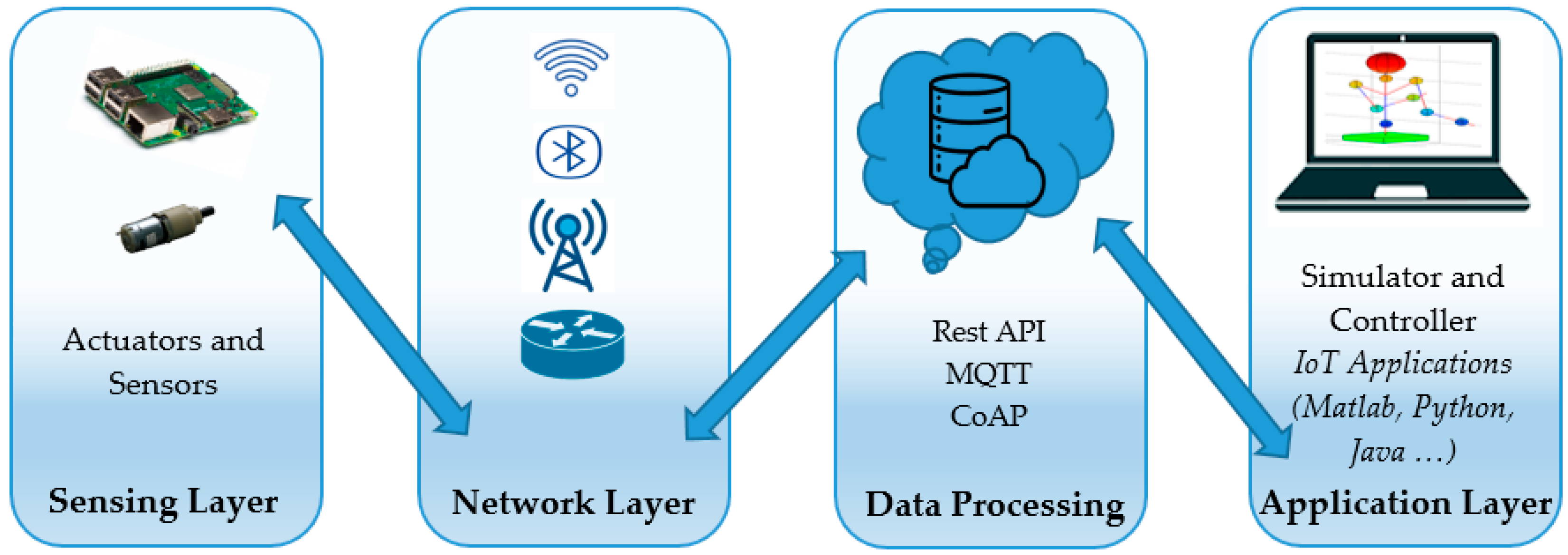
  38. GeeksforGeeks. Architecture of Internet of Things (IoT). GeeksforGeeks. 2024. Available online: https://www.geeksforgeeks.org/architecture-of-internet-of-things-iot/ (accessed on 29 September 2024).
  39. Antoska, V.; Potkonjak, V.; Stankovski, M.J.; Baščarević, N. Robustness of Semi-Humanoid Robot Posture with Respect to External Disturbances. Facta Univ. Ser. Autom. Control Robot. 2012, 11, 99–110. [Google Scholar]
  40. Lagrange Equations (in Mechanics); Encyclopedia of Mathematics; EMS Press: Berlin, Germany, 2001; Available online: https://encyclopediaofmath.org/wiki/Euler-Lagrange_equation (accessed on 20 September 2024).
  41. Weisstein, E.W. Euler-Lagrange Differential Equation. In MathWorld; Wolfram Research, Inc.: Champaign, IL, USA, 2024; Available online: https://mathworld.wolfram.com/Euler-LagrangeDifferentialEquation.html (accessed on 20 September 2024).
  42. Antoska-Knights, V.; Gacovski, Z.; Deskovski, S. Obstacles Avoidance Algorithm for Mobile Robots, Using the Potential Fields Method. Univ. J. Electr. Electron. Eng. 2017, 5, 75–84. [Google Scholar] [CrossRef]
  43. Patil, S.; Vasu, V.; Srinadh, K.V.S. Advances and Perspectives in Collaborative Robotics: A Review of Key Technologies and Emerging Trends. Discov. Mech. Eng. 2023, 2, 13. [Google Scholar] [CrossRef]
  44. Piga, D.; Bemporad, A. New Trends in Modeling and Control of Hybrid Systems. Int. J. Robust Nonlinear Control 2020, 30, 5775–5776. [Google Scholar] [CrossRef]
  45. Roy, S.; Rana, D. Machine Learning in Nonlinear Dynamical Systems. Resonance 2021, 26, 953–970. [Google Scholar] [CrossRef]
  46. Gilpin, W. Generative Learning for Nonlinear Dynamics. Nat. Rev. Phys. 2024, 6, 194–206. [Google Scholar] [CrossRef]
  47. Tang, C.; Abbatematteo, B.; Hu, J.; Chandra, R.; Martín-Martín, R.; Stone, P. Deep Reinforcement Learning for Robotics: A Survey of Real-World Successes. arXiv 2024, arXiv:2408.03539. [Google Scholar]
  48. Han, D.; Mulyana, B.; Stankovic, V.; Cheng, S. A Survey on Deep Reinforcement Learning Algorithms for Robotic Manipulation. Sensors 2023, 23, 3762. [Google Scholar] [CrossRef]
  49. Levine, S. Exploring Deep and Recurrent Architectures for Optimal Control; Stanford University: Stanford, CA, USA, 2013; Available online: https://people.eecs.berkeley.edu/~svlevine/papers/dlctrl.pdf (accessed on 25 September 2024).
  50. Wei, J.; Zhu, B. Model Predictive Control for Trajectory-Tracking and Formation of Wheeled Mobile Robots. Neural Comput. Appl. 2022, 34, 16351–16365. [Google Scholar] [CrossRef]
  51. Silaa, M.Y.; Barambones, O.; Bencherif, A. Robust Adaptive Sliding Mode Control Using Stochastic Gradient Descent for Robot Arm Manipulator Trajectory Tracking. Electronics 2024, 13, 3903. [Google Scholar] [CrossRef]
  52. Schwenzer, M.; Ay, M.; Bergs, T.; Abel, D. Review on Model Predictive Control: An Engineering Perspective. Int. J. Adv. Manuf. Technol. 2021, 117, 1327–1349. [Google Scholar] [CrossRef]
  53. Almassri, A.M.M.; Shirasawa, N.; Purev, A.; Uehara, K.; Oshiumi, W.; Mishima, S.; Wagatsuma, H. Artificial Neural Network Approach to Guarantee the Positioning Accuracy of Moving Robots by Using the Integration of IMU/UWB with Motion Capture System Data Fusion. Sensors 2022, 22, 5737. [Google Scholar] [CrossRef] [PubMed]
  54. Ma, X.; Xu, M.; Li, Q.; Li, Y.; Zhou, A.; Wang, S. 5G Edge Computing: Technologies, Applications and Future Visions; Springer Nature: Berlin/Heidelberg, Germany, 2024; Available online: https://books.google.mk/books?id=zGgFEQAAQBAJ&printsec=frontcover&source=gbs_ge_summary_r&cad=0#v=onepage&q&f=false (accessed on 8 October 2024).
  55. Attaran, M. The Impact of 5G on the Evolution of Intelligent Automation and Industry Digitization. J. Ambient. Intell. Humaniz. Comput. 2023, 14, 5977–5993. [Google Scholar] [CrossRef] [PubMed]
  56. Biswas, A.; Wang, H.-C. Autonomous Vehicles Enabled by the Integration of IoT, Edge Intelligence, 5G, and Blockchain. Sensors 2023, 23, 1963. [Google Scholar] [CrossRef]
  57. Carvalho, G.; Cabral, B.; Pereira, V.; Bernardino, J. Edge Computing: Current Trends, Research Challenges and Future Directions. Computing 2021, 103, 993–1023. [Google Scholar] [CrossRef]
Figure 1. Architecture of the IoT and a robot.
Futureinternet 16 00435 g001
Figure 2. Architecture of mobile robot and code for generating flier object.
Futureinternet 16 00435 g002
Figure 3. Command and control process flowchart for robotic operations.
Futureinternet 16 00435 g003
Figure 4. Hybrid control architecture workflow for robotic systems.
Futureinternet 16 00435 g004
Figure 5. Neural network-based dynamic control system for robotic actuation.
Futureinternet 16 00435 g005
Figure 6. Neural network framework for solving nonlinear dynamics optimization in robotic control.
Futureinternet 16 00435 g006
Figure 7. Block diagram of the control architecture for a mobile robot.
Futureinternet 16 00435 g007
Figure 8. Hybrid control system integrating neural network and traditional control methods.
Futureinternet 16 00435 g008
Figure 9. Distribution of orientation, velocity, and acceleration features in training and test datasets.
Futureinternet 16 00435 g009
Figure 10. Distribution of engineered features reflecting robot dynamics in training and test datasets.
Futureinternet 16 00435 g010
Figure 11. Correlation matrix of orientation, angular velocity, and linear acceleration parameters.
Futureinternet 16 00435 g011
Figure 12. Structure of the neural network model.
Futureinternet 16 00435 g012
Figure 13. Evolution of training metrics over a series of epochs with accuracy and loss.
Futureinternet 16 00435 g013
Figure 14. Position of the robot’s joints during a cart motion with a trapezoidal velocity profile with a distance of 1 m and a time period of T = 3.5 s.
Futureinternet 16 00435 g014
Figure 15. Tracking errors during the cart motion with a trapezoidal velocity profile with a distance of 1 m and a time period of T = 3.5 s.
Futureinternet 16 00435 g015
Figure 16. A detailed visual representation of the simulation: reference ψd and actual ψ course angles and tracking error eψ during the robot’s cart motion with a trapezoidal velocity profile movement.
Futureinternet 16 00435 g016
Figure 17. Position of the robot’s joints during the circular motion with a radius of 1 m and a time period of T = 3.5 s.
Futureinternet 16 00435 g017
Figure 18. Tracking errors during the circular motion with a radius of 1 m and a time period of T = 3.5 s.
Futureinternet 16 00435 g018
Figure 19. A detailed visual representation of the simulation: references and actual trajectories during the robot’s circular motion.
Futureinternet 16 00435 g019
Table 1. Characteristics of cart motion with trapezoidal velocity profile.
Cart Motion with Trapezoidal Velocity Profile
distance (m)4
time (s)3.5
max acceleration (m/s2)6.5
max speed (m/s)1.13
Table 2. Characteristics of circular motion.
Circular Motion
radius/amplitude (m)1
time (s)3.5
max acceleration (m/s2)6.445
max speed (m/s)1.8
Disclaimer/Publisher’s Note: The statements, opinions and data contained in all publications are solely those of the individual author(s) and contributor(s) and not of MDPI and/or the editor(s). MDPI and/or the editor(s) disclaim responsibility for any injury to people or property resulting from any ideas, methods, instructions or products referred to in the content.

