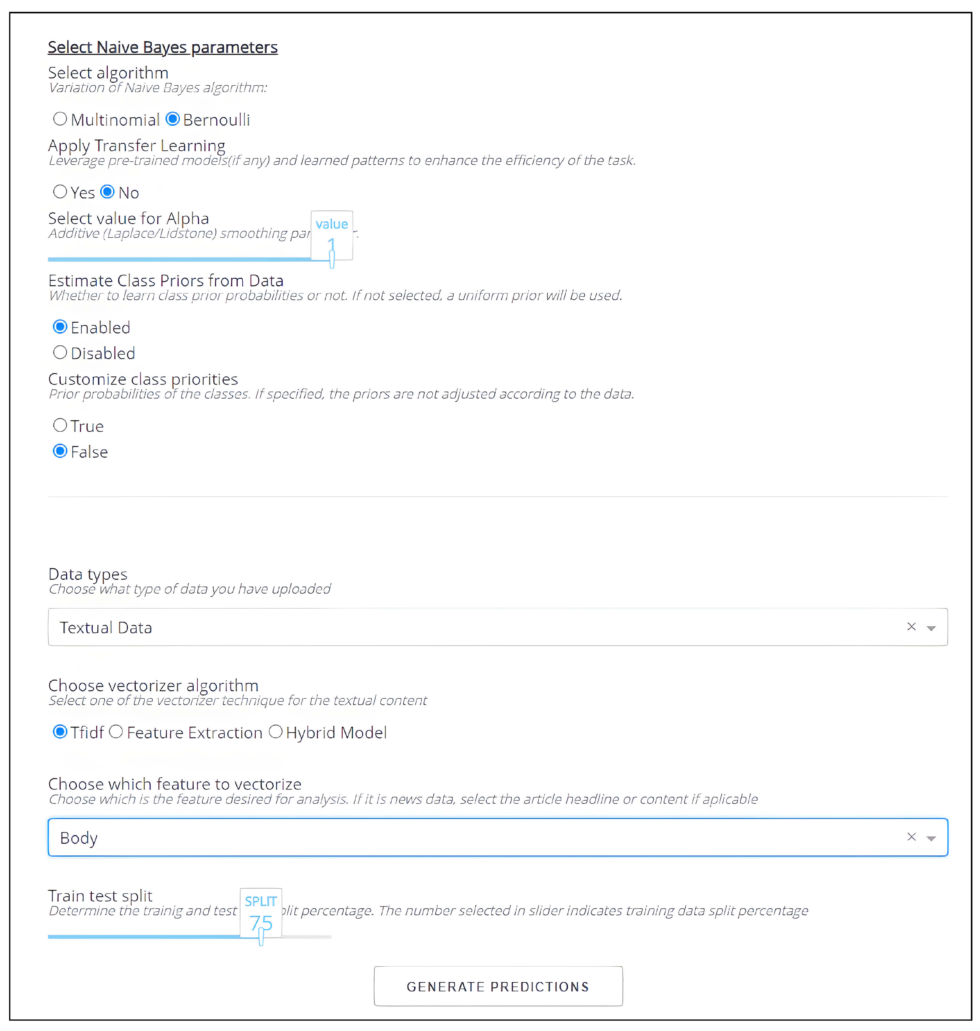
In this work, a total of 24 experiments were conducted to evaluate the performance of various machine learning (ML) models using different settings, datasets, and paradigms.
The first set of twelve experiments compared the performance of all six ML models across three distinct datasets, employing three feature extraction methods. The remaining 12 experiments focused on assessing the potential of transfer and incremental learning using multinomial and Bernoulli naive Bayes classifiers across various datasets.
It is crucial to remember that the overarching objective of these experiments is to highlight the significance of employing the hybrid feature extraction technique.
5.1. Experimental Setup
Each experiment will maintain a standardized setup to ensure a fair and consistent comparison across different models and feature extraction methods.
Dataset Selection: The Merged, Kaggle 1, Kaggle 2, and FA-KES datasets will be used for the first 12 Experiments. Kaggle 2 and Trimmed-Kaggle 1 will be used to train the pre-trained model for transfer learning, and all the
trimmed datasets will be used to train the pre-trained models for incremental learning. These pre-trained models will be tested on larger datasets, namely WELFake, Kaggle 1, and Scraped. The Kaggle 2 dataset and all the
trimmed datasets will also be referred to as the “pre-training” datasets in the following paragraphs. For a complete description and references to these databases, please refer to
Section 3.1.
Train–Test Split: The data within each dataset will undergo a train–test split, employing a 90-10 ratio for the initial 12 experiments. Additionally, 10-fold cross-validation will be executed, with the mean value of each metric calculated. In the subsequent 12 experiments, 95% of the pre-training datasets will be allocated for training the pre-trained models, while 15% of the testing datasets will be utilized for fine-tuning these models.
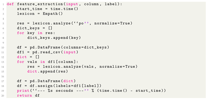
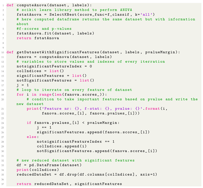
Feature Extraction: Three distinct feature extraction methods will be employed across the first twelve experiments, namely, TF–IDF, Empath, and the novel hybrid approach. The TF–IDF method will be exclusively utilized for the remaining experiments.
Timing: For the first 12 experiments, the Runtime value indicates the time for vectorization and training the models, as we are also comparing the performance between different feature extraction techniques. In the remaining experiments, the Runtime value indicates the time to train (or pre-train and fine-tune) the models.
5.2. Comparing ML Models across Feature Extraction Methods
We explore three feature extraction techniques: TF–IDF, Empath, and our innovative hybrid approach, each paired with six models. Our findings reveal that models utilizing TF–IDF and the hybrid method consistently outperform others (see
Table 1 for results on the Kaggle 1 dataset). Notably, logistic regression shines with an impressive accuracy of 0.96.
Regarding efficiency, the gradient boosting model with the hybrid approach exhibits the longest runtime, clocking in at 256.1 s. Conversely, multinomial naive Bayes (MNB) and Bernoulli naive Bayes (BNB) models leveraging TF–IDF demonstrate the shortest runtimes, both averaging around 11 s.
Furthermore, MNB consistently outperforms BNB across TF–IDF and the hybrid approach, showcasing higher accuracy alongside shorter runtimes.
Like the results from the Kaggle 1 dataset, all models tend to perform better with TF–IDF and the hybrid approach, especially the novel hybrid approach, which yields 99% and 98% accuracy for gradient boosting and logistic regression (see
Table 2 for results on the Kaggle 2 dataset).
Regarding runtime, MNB and BNB are still the fastest among all six models. However, this time, BNB outperformed MNB with a higher value in all four measurements; meanwhile, MNB is still faster than BNB.
All models perform exceptionally well with TF–IDF, particularly decision trees and gradient boosting, achieving near-perfect accuracy and F1 scores (see
Table 3 for results on the Merged dataset). This indicates that almost all predictions are correct. However, KNN lags slightly behind, with accuracy and F1 scores around 0.83. This could be attributed to KNN’s less effective handling of high-dimensional features. BNB and MNB also exhibit strong performance with accuracy and F1 scores in the 0.93–0.94 range.
Except for KNN, all models perform exceedingly well with the hybrid method. Decision trees and gradient boosting models achieve near-perfect accuracy and F1 scores. Logistic regression, BNB, and MNB also show strong performance, with accuracy and F1 scores in the 0.94–0.98 range. Yet, as with the TF–IDF results, KNN is slightly weaker, with accuracy and F1 scores around 0.87.
Meanwhile, Empath is outperformed by the other two feature extraction techniques as in the previous six experiments.
In terms of runtime, gradient boosting takes the longest in all scenarios, particularly with the hybrid feature extraction method, requiring nearly 400 s. This is likely due to its iterative nature, requiring more time to improve its predictions gradually. Conversely, BNB and MNB consistently take the least time across all scenarios, possibly due to their simplicity as models based on naive Bayes theory, with lower computational demands.
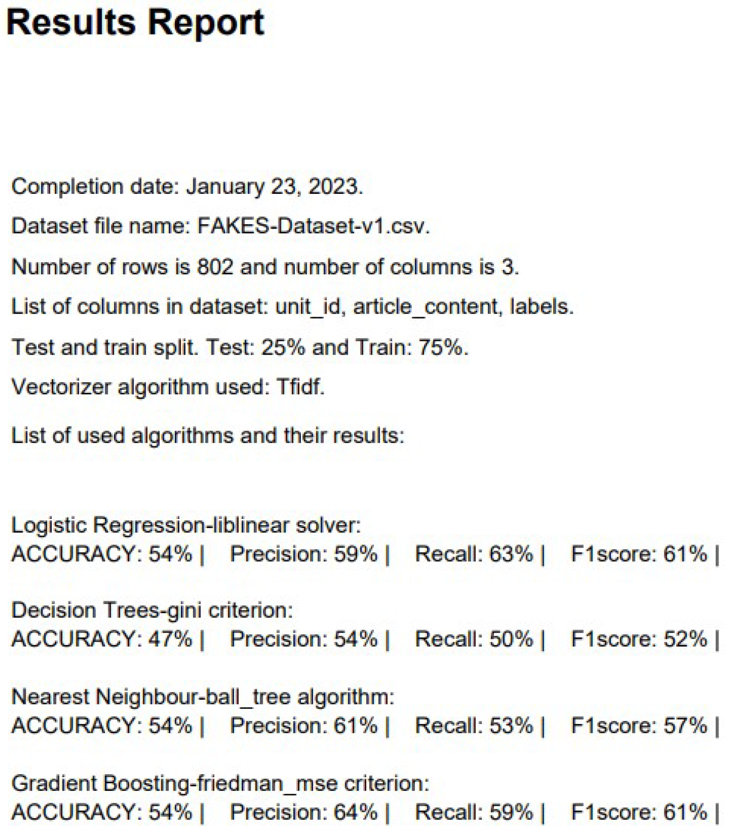
The performance of the models generally declines on the FA-KES dataset, which is smaller in size compared to the first two datasets (see
Table 4 for results on the FA-KES dataset). Regardless of the feature extraction method used, all models’ accuracy lies between 0.45 to 0.57, significantly lower than those on the first two datasets. This might be due to the smaller dataset size, making it harder for the models to learn sufficient patterns for accurate prediction. That is one major reason to consider these results unreliable [
17].
Another point worth noting here is that the MNB model achieved 100% recall with TF–IDF and Empath, meaning that the model recognizes all the news articles as fake. The same happened with LR using Empath. This can also be attributed to the lack of data.
Overall Analysis
Overall, it is evident that logistic regression consistently achieves the highest accuracy across all three datasets, positioning it as the most reliable model for prediction. When time efficiency is a priority, the multinomial naive Bayes (MNB) and Bernoulli naive Bayes (BNB) models stand out, clocking in the shortest runtime.
In terms of feature extraction methods, the hybrid approach invariably enhances all models’ performance. However, this comes with the trade-off of a considerably longer runtime. The TF–IDF method, on the other hand, provides a favorable balance between performance and speed, yielding respectable accuracy in a relatively short time.
An interesting dynamic is seen between MNB and BNB models. MNB shows superior performance when dealing with larger datasets, while BNB takes the lead in the context of smaller data volumes; ref. [
33] demonstrates the importance of choosing the right model based on the specific characteristics of the dataset.
5.3. Results and Discussion on Transfer Learning
5.3.1. Pre-Training on Kaggle 2 for Testing on Kaggle 1
In
Table 5 and
Table 6, we show the results we obtained from training our models on the Kaggle 2 database and then testing on the Kaggle 1 database. It is worth noting that the time taken for training the pre-trained model was 0.0083 s (BNB) and 0.0059 (MNB). While both models exhibited a minor dip in accuracy, fine-tuning the pre-trained models proved significantly more time-efficient than training a new model from the ground up. Specifically, the Bernoulli naive Bayes (BNB) model demonstrated a speed increase by a factor of seven, while the multinomial naive Bayes (MNB) model was six times faster. This represents a considerable advantage, underscoring the potential benefits of leveraging pre-trained models in terms of computational efficiency [
22].
In order to demonstrate the significance of transfer learning, we conducted a one-time experiment wherein we trained a model and saved it to a pickle file. We then directly applied this pre-trained model to a new dataset without utilizing transfer learning (
Table 7).
From these results, it can be noted that the performance of the models was notably diminished when applied to a new dataset without transfer learning. These results underpin the importance of transfer learning when applying pre-trained models to new datasets, highlighting its role in maintaining and potentially improving model performance.
It is important to note that this process was carried out only once for illustrative purposes and will not be repeated for each experiment in the project. The key takeaway from this experiment is the crucial role of transfer learning in ensuring the generalization capability of machine learning models.
5.3.2. Pre-Training on Kaggle 2 for Testing on FA-KES
In
Table 8 and
Table 9, we show the results we obtained from training our models on the Kaggle 2 database and then testing on the FA-KES dataset.
From the results tables, it is clear that the application of transfer learning to the FA-KES dataset did not lead to any significant improvements. Notably, the recall for the MNB model remains at 1 in both scenarios, indicating that the model has classified every news article in the dataset as fake. The previous experiment also observed this phenomenon, leading to concerns about the model’s validity. As such, these results have been deemed unreliable, prompting us to disregard them in our analysis.
5.3.3. Pre-Training on Trimmed-Kaggle 1 for Testing on Kaggle 2
In
Table 10 and
Table 11, we show the results we obtained from training our models on the Trimmed-Kaggle 1 dataset and then testing on the Kaggle 1 database. It is worth noting that the time taken for training the pre-trained model was 0.014 s (BNB) and 0.006 s (MNB).
Based on the results we have obtained, the application of transfer learning on the Kaggle 2 dataset has actually decreased model performance rather than enhancing it. This significant reduction in performance indicates that the transfer learning experiment was not successful in this context. It is possible that the pre-trained model did not align well with the Kaggle 2 dataset. Therefore, this experiment can be deemed unsuccessful, highlighting the importance of ensuring compatibility between the pre-training and target tasks in a transfer learning scenario [
23].
5.3.4. Overall Analysis
The results from these experiments demonstrated that while transfer learning significantly enhances computational efficiency, its effectiveness in improving model performance varies based on the dataset used. In our case, an improvement in model performance was observed when testing on the Kaggle 1 dataset, but the application of transfer learning led to a reduction in performance for the Kaggle 2 dataset and yielded unreliable results on the FA-KES dataset.
These findings highlight the importance of dataset compatibility in transfer learning applications. It also underscores the need to consider the specific characteristics of the datasets when designing machine learning systems, as the success of transfer learning appears to be highly dependent on the similarity between the pre-training and target tasks.
5.4. Results and Discussion on Incremental Learning
In this section, we delve into the results of three experiments centered around incremental learning.
5.4.1. Pre-Training on Trimmed-Kaggle 1 for Testing on Kaggle 1
In
Table 12 and
Table 13, we present the results obtained with and without incremental learning. Notably, the pre-trained model required 0.014 s for training in the case of BNB and 0.006 s for MNB.
Both models utilizing incremental learning techniques exhibited superior performance compared to those trained from scratch. Despite requiring a similar time investment for fine-tuning as transfer learning, they demonstrated significantly higher accuracy. This improvement can be attributed to the alignment between the pre-training dataset and the final testing dataset. Leveraging this alignment allowed the models to more effectively learn and generalize, resulting in enhanced accuracy. This observation is supported by the findings of Schlimmer (1986) [
30].
5.4.2. Pre-Training on Trimmed-WELFake for Testing on WELFake
In
Table 14 and
Table 15, we present the results obtained with and without incremental learning. Notably, the pre-trained model required 0.009 s for training in the case of BNB and 0.004 s for MNB.
The results demonstrate that implementing incremental learning on the WELFake dataset with both the BNB and MNB models leads to a decrease in runtime without a substantial compromise in performance. Prior to incremental learning, the BNB and MNB models achieved accuracy scores of 0.9 and 0.86, respectively, but incurred relatively higher runtimes at 0.14 and 0.06.
Upon implementing incremental learning, there was a slight reduction in accuracy, yet the runtime significantly improved to 0.028 and 0.01, respectively. This underscores the advantage of incremental learning in enhancing computational efficiency, particularly valuable in scenarios where computational resources or time constraints exist.
5.4.3. Pre-Training on Trimmed-Scraped for Testing on Scraped
In
Table 16 and
Table 17, we present the results obtained with and without incremental learning. Notably, the pre-trained model required 0.008 s for training in the case of BNB and 0.003 s for MNB.
The experimentation conducted with the Scraped dataset yielded mixed outcomes upon the implementation of incremental learning. While there was a notable improvement in runtime for both the BNB and MNB models, the performance metrics displayed significant fluctuations.
To elaborate, focusing on the Bernoulli naive Bayes (BNB) model, there was an enhancement in accuracy, rising from 0.77 to 0.82, alongside a reduction in runtime from 0.035 to 0.0114. Despite these relatively minor adjustments, they imply that incremental learning may offer advantages for this specific model.
Conversely, the multinomial naive Bayes (MNB) model experienced a substantial decrease in performance, with accuracy plummeting from 0.76 to 0.58. This emphasizes that the benefits of incremental learning may not be consistent across all models or datasets.
The discrepancy in performance is further underscored by the MNB model’s high precision but low recall score post incremental learning. This suggests that while the model correctly identifies positive instances (high precision), it fails to identify all positive instances (low recall), particularly regarding the classification of fake news. This inclination toward conservative labeling, where news articles are labeled as false only when the model is highly certain, may contribute to the observed decrease in accuracy.
One plausible explanation for these findings is rooted in the essence of incremental learning. This approach operates under the assumption that the model receives regular updates with new data. However, if the incoming data deviates from the overall distribution of the dataset or introduces novel concepts unfamiliar to the model, classification accuracy may suffer.
This observation aligns with the Scraped dataset’s characteristics, comprising news articles sourced from diverse web sources through web crawlers. Given this diversity, it is conceivable that the incoming data may not align closely with the distribution or features of the initial data used for model pre-training.
The overall analysis of the experiments with incremental learning highlights its potential to enhance computational efficiency, evidenced by reduced runtimes across all cases. However, its impact on model performance varied depending on the dataset and the model under consideration.
Incremental learning yielded improved accuracy for both models when tested on the Kaggle 1 dataset, attributed to the robust alignment between the pre-training and final testing datasets. Conversely, its application to the WELFake dataset led to a slight decrease in performance despite the observed enhancement in runtime efficiency.
Of particular interest is the disparate impact of incremental learning on the two models when applied to the Scraped dataset. While the Bernoulli naive Bayes (BNB) model showed marginal accuracy improvements, the multinomial naive Bayes (MNB) model experienced a notable decline in performance. This discrepancy could be attributed to inconsistencies between the data used for pre-training the model and the subsequent fine-tuning data.
These findings underscore that the benefits of incremental learning are not universally applicable and necessitate careful evaluation based on the specific characteristics of the models and datasets involved. Particularly for diverse datasets like Scraped, the advantages of incremental learning may be constrained due to the heterogeneous nature of incoming data.
