1-D Convolutional Neural Network-Based Models for Cooperative Spectrum Sensing

Abstract

Spectrum sensing is an essential function of cognitive radio technology that can enable the reuse of available radio resources by so-called secondary users without creating harmful interference with licensed users. The application of machine learning techniques to spectrum sensing has attracted considerable interest in the literature. In this contribution, we study cooperative spectrum sensing in a cognitive radio network where multiple secondary users cooperate to detect a primary user. We introduce multiple cooperative spectrum sensing schemes based on a deep neural network, which incorporate a one-dimensional convolutional neural network and a long short-term memory network. The primary objective of these schemes is to effectively learn the activity patterns of the primary user. The scenario of an imperfect transmission channel is considered for service messages to demonstrate the robustness of the proposed model. The performance of the proposed methods is evaluated with the receiver operating characteristic curve, the probability of detection for various SNR levels and the computational time. The simulation results confirm the effectiveness of the bidirectional long short-term memory-based method, surpassing the performance of the other proposed schemes and the current state-of-the-art methods in terms of detection probability, while ensuring a reasonable online detection time.

1. Introduction

With the rapid growth of diverse technologies and the proliferation of systems and wireless communication devices, there is a rising need for radio spectrum. An an example, billions of items already proliferate in the Internet of Things (IoT) ecosystem [1], leading to novel application domains such as Smart Cities [2], from an all-embracing perspective including variant sub-applications, Industry 4.0, e-government, and others [3]. The availability of radio spectrum has become limited as it is a precious resource. Moreover, statistics from the Federal Communications Commission (FCC) indicate that the existing fixed spectrum allocation policy has led to the inefficient utilization of licensed spectrum bands [4]. Therefore, cognitive radio (CR) [5] has emerged as a promising technology that incorporates intelligent spectrum management techniques to effectively utilize frequency bands in specific times and locations (known as spectrum gaps or, more generically, white spaces) when not in use by licensed users [6,7]. In this situation, unlicensed users can transmit their signals with the understanding that the transmission of licensed users is adequately safeguarded. This is accomplished through a procedure known as spectrum sensing (SS), which involves the detection and analysis of the radio frequency (RF) environment [8,9]. Spectrum sensing entails checking whether the licensed user (primary user—PU) is currently transmitting, thereby enabling the unlicensed user (so-called secondary user—SU) to transmit their signals.

Conventional SS methods, such as energy detection and matched filtering, struggle to cope with the variability and complexity of real-world wireless environments. The reliability of spectrum sensing is affected by signal fading, shadowing and the presence of various types of interference. Traditional SS algorithms cannot adequately adapt to these challenges, leading to inaccurate or delayed spectrum occupancy detection. Moreover, they usually fail to take full advantage of the temporal, frequency or spatial dependencies that exist in the detected signals, resulting in rather limited performance [10,11,12]. Machine learning (ML) techniques have demonstrated significant potential in improving the performance of spectrum sensing. By leveraging ML algorithms, CR networks can learn and adapt to the dynamics of the radio frequency (RF) environment, enhancing the accuracy of spectrum occupancy detection and reducing false positives. Accordingly, researchers have recently turned their attention to ML algorithms for signal sensing [13,14].

In the context of ML algorithms, deep neural networks (DNNs) excel at learning intricate patterns and representations from data, making them suitable for a wide range of recognition/classification tasks, and, specifically, for spectrum sensing. Deep learning (DL) methods, particularly recurrent neural networks (RNNs), have emerged as the most widely adopted machine learning algorithms. RNNs are renowned for their capability to leverage historical data in order to make precise predictions about the future or current state. RNN algorithms are utilized in [15], where the authors use a signal covariance matrix-based SS algorithm and long short-term memory (LSTM) to jointly extract the spatial cross-correlation features of multiple signals received by the antenna array and the temporal autocorrelation features of single signals.

The individual detection performed by each SU using ML is computationally complex and can be inaccurate. Indeed, ML algorithms require a large amount of training data to be able to recognize the temporal, frequency and location dependencies that exist in the transmitted and received signal. The end-user terminal usually does not have sufficient computing and memory resources to store and process the volumes of data needed to train an ML algorithm. As discussed earlier, a common idea is to use cooperative sensing, in which SUs share their sensing results or collected data to cooperatively decide the current state of the spectrum. This approach solves the problem of generating an ML model, which can be created by the end user’s elected device or by the so-called “fusion center” or a “central server”. ML has also shown utility in cooperative sensing, where multiple sensing nodes attempt to establish the state of the spectrum [16,17]. To share SUs’ sensing results or collected data with the fusion center and to receive a spectrum occupancy decision, bidirectional wireless communication will be implemented between each SU and the fusion center. These communications will be supported by a real wireless channel and, accordingly, they can be affected by imperfect transmission. We will take these imperfections into account when evaluating the performance of the proposed approaches.

Following these observations and taking them into account, we propose three distinct schemes of a cooperative spectrum sensing (CSS) algorithm based on a deep neural network (DNN) model. Our approaches are specifically designed for a multi-antenna, multi-SU scenario, aiming to leverage the capabilities of both one-dimensional convolutional neural networks (1DCNN) and long short-term memory (LSTM) networks at the SU level. By combining these networks, we can effectively extract both local and global features from sequential data, enabling the learning of group-level PU activity patterns for accurate classification. We opt for the 1DCNN due to its remarkable ability to extract local features from sequential data. Additionally, the incorporation of LSTM layers enhances the extraction of global correlations, further improving the overall performance of the model. To evaluate the effectiveness of our proposed model, we consider the impact of both imperfect reporting and imperfect detection channels, demonstrating its robustness in challenging scenarios.

The rest of this paper is structured as follows. In Section 2, we introduce the related work for this paper. An overview of the SS principle and adopted DL algorithms is provided in Section 3. Section 4 presents a detailed description of the proposed model based on DL. In Section 5, we present the verification of this solution, and we discuss the computer simulation details. Finally, we summarize this contribution in Section 6.

2. Related Works

The conventional approaches for SS can be classified into three main groups, which are energy detection [18], feature-based detection [19] and matched filter detection (MFD) [20]. The latter utilizes a predefined filter to conduct correlation operations between known and unknown signals, aiming to detect specified frequency and modulation signals effectively. One notable advantage of this approach is its ability to achieve a low probability of false detection in a short time. However, it does require perfect knowledge of the primary user’s signaling features, which is not obligatory for primary users, and it involves substantial power consumption. As a result, MFD is often deemed suitable for scenarios with known master user signal information and high-phase synchronization. Generally, SS approaches require prior knowledge about the PU’s signal or noise power, but this prior knowledge may not be available in many cases, especially for non-cooperative communication [21]. Therefore, the literature primarily focuses on blind detection techniques, which are suitable for a diverse range of SS scenarios in dynamic environments, without requiring this information. Energy detection (ED) is a commonly used technique due to its ease of implementation [22]. It operates by measuring the energy levels of the received signal in a particular frequency band and comparing them to a predefined threshold value to determine whether the band is occupied by a primary user or not. However, energy detection suffers from noise uncertainty [23]. It is suitable for spectroscopic detection tasks in low-SNR environments but often requires combination with other signal identification and analysis techniques due to its susceptibility to false alarms and reduced sensitivity in high-noise environments. To address this issue, maximum eigenvalue detection (MED) has been proposed [24,25], which involves calculating the eigenvalues and dynamically adapting the detection threshold based on the expected minimum energy level of the primary user signal. MED stands out for its heightened sensitivity to signal changes by focusing on detecting the largest eigenvalue. This characteristic makes it particularly effective in capturing variations in signal characteristics, enhancing its utility in scenarios where subtle changes are significant. Despite its advantages, the practical application of maximum eigenvalue detection encounters challenges in certain scenarios, such as environments characterized by high dynamics or non-linear signal behavior, where its performance may degrade. Nevertheless, this method finds utility when dealing with signals in which changes in the largest eigenvalue signify meaningful variations, providing a reliable means to discern significant signal characteristics across a range of applications. In [24], the authors compare the performance of MED and ED in different scenarios and demonstrate that MED outperforms ED in scenarios with a low SNR and high noise levels. Another widely used method is cyclostationary detection, which leverages the statistical characteristics of modulated signals to demonstrate the periodicity of detection. This method showcases more stable performance in the presence of background noise uncertainty and can operate effectively under low SNR conditions. Nevertheless, it is important to acknowledge that the performance of cyclostationary feature detection may be compromised if the received signal exhibits cyclostationary features due to background noise. Additionally, the computation time and complexity associated with Fourier transforming the cyclical autocorrelation function need to be considered when implementing this method. Nevertheless, traditional sensing methods have limitations in their ability to fully exploit the time, frequency or spatial dependencies that exist in the detected signals. As a result, their performance may be limited in certain scenarios.

Researchers have delved into inventive approaches harnessing the power of machine learning. Among these methods, the K-means algorithm, widely adopted for the clustering of data, has demonstrated its effectiveness in grouping data into adjacent partitions based on similar features [26,27]. In [28], a new spectrum sensing method based on the empirical mode decomposition algorithm and K-means clustering algorithm is proposed to solve the problems related to the poor performance of traditional spectrum sensing methods under low signal-to-noise ratios. A blind multi-band spectrum sensing method requiring no knowledge of the noise power, primary signal and wireless channel is proposed based on the K-means clustering in [29]. In this approach, the K-means clustering algorithm is used to identify the occupied sub-band set and the idle sub-band set.

Deep learning is a promising approach to enhancing the detection performance and supporting blind sensing, as DL models can automatically extract relevant features and patterns from data that are difficult or impossible to detect using traditional methods [30,31]. Peng et al. [32] utilized a CNN for SS, using transfer learning from computer vision to improve the detection of various signal types. Similarly, transfer learning has been applied to a residual neural network (ResNet) model for this purpose [33]. Gao et al. [34] combined an LSTM network with a CNN to capture global dependencies and local features from time series data, outperforming separate RNN and CNN structures. Yang K. et al. [35] proposed a blind SS method based on DL that used an end to end 1DCNN and LSTM network structure. This method showed better performance than an energy detector, especially when the signal-to-noise ratio was low, and it showed the potential to significantly enhance the performance of cognitive radio networks (CRNs) in terms of efficient detection.

Individual SS, where each radio device independently monitors the spectrum to detect unused or available sub-bands, has some limitations that can lead to problems in efficient spectrum usage [36]. To address these problems, the authors of [37] proposed a CNN-based CSS technique that extracts features from the observed signal to enhance the sensing performance, considering three classical CNN-based CSS schemes: LeNet, AlexNet and VGG-16. The simulation results demonstrated that the proposed schemes achieved significantly improved sensing accuracy compared to traditional ones. Soni B. et al. [38] proposed an LSTM-based SS method that learns implicit features from the spectrum data, such as temporal correlations using PU activity statistics, and it achieved improved detection performance and classification accuracy at low signal-to-noise ratios. In the same context of CSS, Xu M. et al. [39] proposed a multi-feature combination network, which simultaneously extracts spatial and temporal features through a parallel structure that leverages the complementary modeling capabilities of 1DCNN and gated recurrent unit (GRU) networks. The experimental results indicated that the proposed approach achieved competitive performance. In [40], a hybrid CNN-LSTM architecture for CSS was proposed, demonstrating high detection accuracy and reduced complexity compared to other DL-based methods. To further improve the detection performance, a hierarchical cooperative LSTM-based CSS method was proposed in [17] to learn the PU activity pattern at both the SU level and group level. The simulation results showed that this method outperformed the state-of-the-art approaches in terms of detection probability and classification accuracy. To overcome the limitations of the traditional CNN and LSTM [41,42], Xing H. et al. [43] proposed a deep neural network model that incorporates a two-layer 1DCNN, bidirectional LSTM and self-attention (SA) techniques. The 1DCNN extracts local patterns from a given time series, while BiLSTM mines long- and short-period dependencies in opposite directions. The SA helps to relate the features at specific positions of the time series, leading to improved performance. While deep learning-based spectrum sensing offers high accuracy and adaptability to complex and dynamic environments, it is not without its drawbacks. The requirement for a large amount of labeled data and substantial computing resources for training can be prohibitive. Moreover, issues related to interpretability and transparency in deep learning models remain a challenge, making it difficult to understand the decision-making process and trust the outcomes, especially in critical applications. Furthermore, when it comes to deep learning-based spectrum sensing, the focus on single-node detection poses its own set of challenges. Deep learning models, often trained on centralized datasets, can struggle to adapt seamlessly to diverse, decentralized sensing environments. The ability to capture nuanced patterns and spectrum variations between different nodes becomes crucial to ensure the effectiveness of these models in real-world scenarios, where nodes may exhibit distinct signal characteristics. Nevertheless, overfitting is a common concern in deep learning, especially when dealing with complex architectures. Regularization techniques, though beneficial, require careful tuning to strike a balance between preventing overfitting and preserving model performance.

Federated learning (FL) and federated reinforcement learning (FRL) frameworks can be successfully applied in order to take advantage of knowledge sharing without leading to problems of privacy and network overloading [44,45]. An FL framework for CSS was proposed in [46]. This framework can perform collaborative training while ensuring local data privacy and greatly reducing the traffic load between the SUs and fusion center. In [47], the authors proposed a spectrum access model based on the federated deep Q network (DQN), which adopts the asynchronous federated weighted learning algorithm to share and update the weights of the DQN in multiple agents, to decrease the time cost and accelerate convergence. The decentralized nature of FL comes with its own set of challenges. Coordinating computations across many nodes is a major challenge, particularly in scenarios where devices may have different computational capabilities and network conditions. The need to aggregate model updates introduces a communication overload, which can lead to increased latency and resource consumption, which is a critical consideration in real-time spectrum sensing applications. This communication overhead becomes a critical consideration in ensuring the efficiency of FL implementations. FL relies on decentralized data across multiple devices, addressing privacy concerns by keeping sensitive information local. However, data diversity between nodes becomes crucial. Imbalances or biases in the data distribution may impact the federated model’s ability to generalize effectively to different spectral conditions. In addition, the collaborative nature of federated learning, with models trained on diverse datasets across nodes, introduces challenges in managing overfitting. Striking a balance between model convergence and overfitting prevention becomes a delicate exercise. Ensuring that the federated model converges collectively without sacrificing performance on individual nodes requires the careful consideration of the hyper-parameters and regularization techniques to maintain robustness and generalization capabilities.

In this paper, we propose three distinct DNN schemes tailored to CSS in a multi-antenna and multi-SU device scenario. These schemes have been carefully designed to address the specific requirements of the scenario. Motivated by the need to reduce the amount of data transmitted and maintain the privacy of the information, as mentioned in [42,43], we have incorporated these components into our network designs. The proposed designs in our work represent an enhancement in terms of accuracy, rapidity and computational efficiency for secondary user (SU) devices in cooperative spectrum sensing, all while ensuring privacy protection. An essential feature of our models is their privacy-centric approach. Instead of transmitting raw data, which may contain sensitive information, the models send only the model weights as a vector to the fusion center as the signals are processed at the SU level. This vector representation preserves the privacy of the SU devices while still enabling effective cooperative spectrum sensing. This not only accelerates the detection time but also optimizes the computational resources, making our designs more efficient for resource-constrained SU devices. In contrast to conventional cooperative spectrum sensing approaches that may involve transmitting raw data or detailed information, our vectorized model weight transmission minimizes information exchange, reducing the risk of privacy breaches. This streamlined communication contributes to the models’ rapidity and computational efficiency. By leveraging the strengths of 1DCNN and LSTM/BLSTM, we aim to enhance the performance of our CSS system. It is crucial to emphasize that while we have taken inspiration from the mentioned references, our proposed hyper-parameters and network architectures are distinct and carefully designed to cater to the specific challenges encountered in the CSS of the proposed scenario. Specifically, we propose vectorizing multi-antenna data into a one-dimensional format, which can facilitate processing and analysis using machine learning models. This approach can also improve the memory efficiency by significantly reducing the memory overhead and decreasing the memory footprint compared to artificially expanding the data to higher dimensions. This memory efficiency arises from data preprocessing techniques and the model architecture. The presence of fewer parameters means that less memory is required to store the model’s weights and intermediate activations during training, resulting in lower memory usage during forward and backward passes in the training process. This advantage is particularly significant when working with limited computational resources, making it a practical choice, especially in resource-constrained environments.

3. Overview of Spectrum Sensing and Adopted Deep Learning Algorithms

Deep learning algorithms have demonstrated significant performance in the corresponding tasks compared to conventional methods, mainly CNN and RNN algorithms, which are complementary in their modeling capabilities. For the purpose of realizing SS based on a hierarchical DL network, in the subsequent subsections, we briefly introduce the basic concepts of spectrum sensing, the multilayer perceptron, convolutional neural networks and bidirectional long short-term memory.

3.1. Spectrum Sensing Principle

Spectrum sensing is the task of obtaining awareness about the spectrum usage and existence of primary users in a geographical area. This awareness can be obtained by using geolocation and datasets, by using beacons or by local SS at cognitive radios [6]. Thereafter, the system detects the unoccupied spectrum in a timely manner according to the spectrum utilization characteristics. The reuse of the non-renewable spectrum is achieved by allowing cognitive radios to opportunistically access underutilized frequency bands. In the context of a centralized cooperative CRN comprising multiple multi-antenna SUs, we can formulate a binary hypothesis testing problem to determine the presence or absence of a primary user. We consider two hypotheses: $H_1$ represents the active state of the PU, indicating that its transmission is ongoing, while $H_0$ represents the inactive state of the PU, indicating its non-transmission or idle state. The received signal $x_s^m\left(n\right)$ at the m-th antenna of the s-th SU can be formulated as follows:

$${\left\{x_s^m\left(n\right)\right\}}_{n=1}^N=\left\{\begin{array}{cc}{\left\{w_s^m\left(n\right)\right\}}_{n=1}^N\hfill & H_0\hfill \\ {\{h_s^m\left(n\right)s\left(n\right)+w_s^m\left(n\right)\}}_{n=1}^N\hfill & H_1\hfill \end{array}\right.$$

(1)

where $s\left(n\right)$ denotes the PU signal and $w_s^m$ denotes the noise signal received at the m-th antenna of the s-th SU. $h_s^m$ represents the channel gain between the PU and the m-th antenna of the s-th SU. When the sensing interval is shorter than the channel coherence time, the channel gain remains constant and stable within this interval. However, across multiple sensing intervals, the channel gain undergoes fading, which refers to variations in the strength or quality of the channel. This fading is modeled using a statistical distribution that characterizes the variations in channel gain over time. To evaluate SS techniques, two criteria are considered: the detection probability ($P_d$) and the probability of false alarms ($P_{fa}$). The detection algorithm’s performance is usually indicated by these two metrics:

$$\begin{array}{c}\hfill P_{fa}=Prob\{T>\lambda \mid H_0\}\\ \hfill P_d=Prob\{T>\lambda \mid H_1\}\end{array}$$

(2)

The statistical test of the detector, denoted as T, is compared to a threshold value $\lambda$ to make a decision. $P_{fa}$ represents the probability that the test falsely declares that the band under consideration is occupied. $P_d$ denotes the probability that the PU is actually transmitting on the band under consideration when the result of the test is positive. The performance of a detector can be evaluated by plotting its receiver operational characteristic (ROC) curve. This is a graphical depiction of detection probability $P_d$ against false alarm probability $P_{fa}$ for different threshold levels.

3.2. Deep Neural Networks

Artificial neural networks (ANNs) are structures that take inspiration from the functioning of the human brain. They have the ability to estimate the function of a model and process linear/non-linear functions by learning from the relationships between data and applying this knowledge to new situations. One of the most commonly used ANNs is the multilayer perceptron (MLP), which is a type of feedforward ANN where information flows in one direction only, from the input layer to the output layer, passing through the hidden layers. Each layer, except for the input layer, contains computational units, known as neurons, which compute the weighted sum of the connections between neurons and pass through an activation function to introduce non-linearity to the model [48].

In the forward pass, the input values progress through the network’s layers, typically as a multidimensional vector; the input of each neuron in each layer is multiplied by its corresponding weight and then summed. This sum is then passed through a nonlinear activation function, such as ReLU or Sigmoid [49], before being sent to the next layer as input. The equation for the forward pass of a neuron in layer l, taking inputs from layer $l-1$, can be written as

$$y_j^{\left(l\right)}=g\left(h_j^{\left(l\right)}\right)=g\left(\sum _{k=1}^K{\omega }_{jk}{y}_k^{(l-1)}-b_j\right)$$

(3)

where j is a specific neuron of the considered layer l, $g\left(x\right)$ is a nonlinear activation function, h is the dot product of the weights and inputs of the neurons in the previous layer, K denotes the number of neurons in the previous layer, b denotes the bias and ${\omega }_{jk}$ is the synaptic weight between the neurons $k=1\dots K$ in the previous layer $l-1$ and the specific j neuron of the layer l. At the end of the forward propagation, the output $y_j^{\left(L\right)}$ of each neuron j in the output layer L is obtained. At the end of the forward process, the output obtained is then compared with the expected output for this sample to determine the loss function J. The gradients of the loss function with respect to the weights and biases can be calculated using backpropagation (BP). This process involves calculating the derivative of the activation function and propagating the error contributions from the subsequent layers back to the earlier layers. By iteratively updating the weights and biases based on these gradients, utilizing an optimization algorithm such as gradient descent, the loss in the prediction model is gradually decreased until a predetermined stopping criterion is satisfied. BP can make use of a number of gradient descent optimization methods, notably stochastic gradient descent (SGD), momentum SGD [50], AdaGrad [51] Adam and RMSprop and its variants [52,53]. The MLP approach has proven to be effective in SS because it automatically extracts features from the spectrum data, which improves the detection accuracy. In [54], MLP was compared to support vector machines and conventional SS methods in a CSS context, and the results showed that MLP had a better balance between the training time and channel detection performance.

A DNN is a type of artificial neural network with multiple layers between the input and output layers. It is considered “deep” because of the depth of the network, referring to the numerous layers through which data are transformed. Multiple hidden layers allow it to learn hierarchical representations of the data. Various deep learning architectures use deep neural networks, including convolutional neural networks (CNNs) for image processing, recurrent neural networks (RNNs) for sequential data and Transformer models for natural language processing. In the context of this paper, we exploited both the CNN and RNN architectures for the goal of cooperative spectrum sensing and we compared the performance of the proposed approaches.

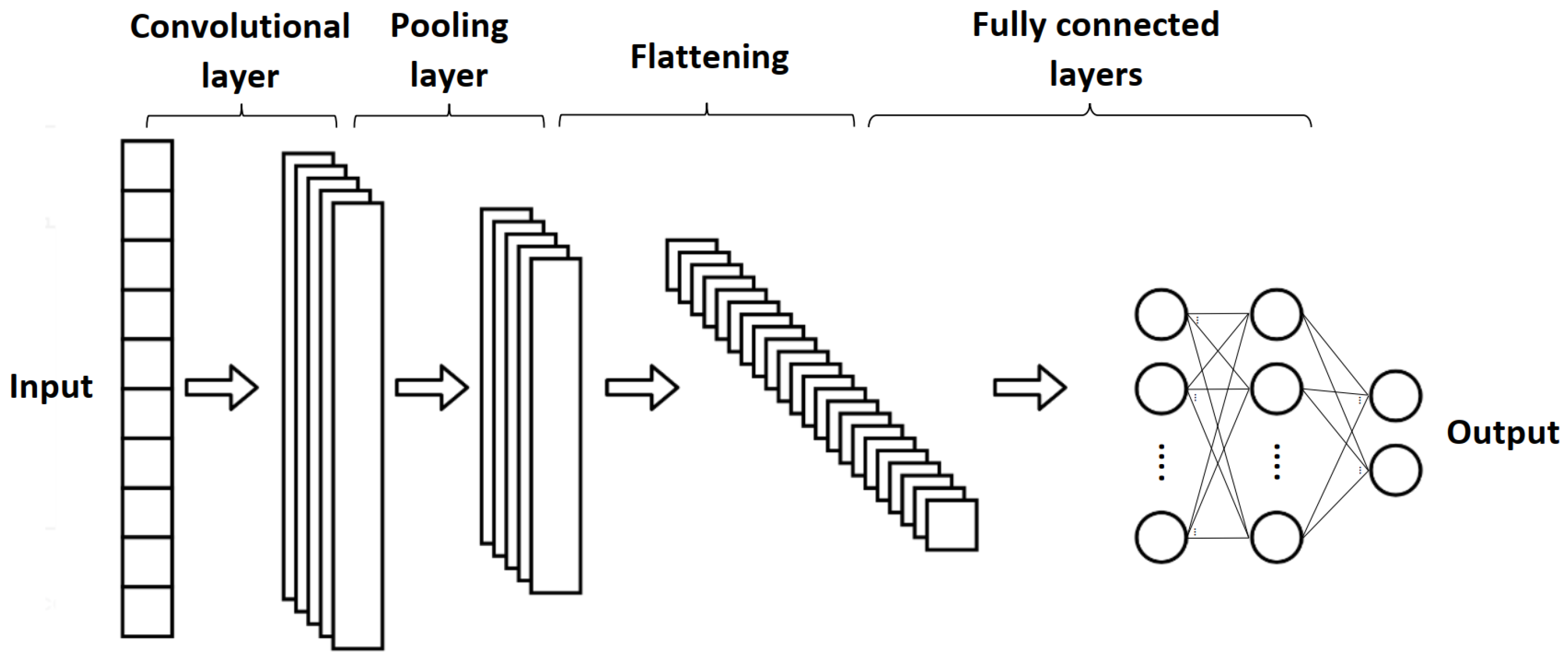
3.3. One-Dimensional Convolutional Neural Network

Convolutional neural networks are a type of DNN used to process data in multiple arrays, such as images. The key feature is the use of convolutional layers, which apply a set of filters to the input data, extracting relevant features and patterns. This allows image-specific features to be incorporated into the network design, improving the performance for image-based tasks and reducing the configuration parameters. CNNs are based on four key concepts that exploit the properties of natural signals: local connections, shared weights, pooling and multiple layers [30]. CNNs are renowned for their significant computational demands, necessitating specialized hardware, particularly during the learning process. As a result, real-time applications on mobile devices and devices with limited power and memory resources should refrain from employing 2DCNNs. Furthermore, achieving a satisfactory level of generalization in deep CNNs requires a sufficiently large dataset for training. However, in many real-world applications involving 1D signals, acquiring labeled data can be challenging, making this approach less feasible. A modified version of a CNN, called 1DCNN, has recently been developed. Studies have shown that for some applications, 1DCNNs are advantageous and therefore preferable to their 2D counterparts for 1D signal processing [32,55]. In particular, 1DCNNs use three main types of layers: convolutional layers, pooling layers and fully connected layers. Figure 1 shows a streamlined 1DCNN architecture for classification.

The initial step in 1D filter kernels involves a series of convolutions, whose sum passes through the activation function, followed by a pooling operation that reduces the output of each convolutional layer. This sets apart 1DCNNs from 2DCNNs, where 2D matrices are used for kernels and feature maps. In the subsequent stage, the CNN layers work on the raw 1D data and “learn to extract” the features required for classification, which is accomplished by the fully connected (FC) layers. They establish connections between each neuron and the neurons in the preceding layer, enabling intricate interactions and the integration of information from various features. FC layers perform a weighted sum of the inputs, followed by an activation function, resulting in the final output. As a result, the process of feature extraction and classification is combined into a single backpropagation process, allowing for optimization to enhance the classification accuracy. This integration is a key advantage of 1DCNNs. Additionally, 1DCNNs can minimize the computational complexity compared to 2DCNNs since the primary operation involves a sequence of 1D convolutions, which inherently have lower dimensionality. A 1DCNN involves simpler filter operations with fewer parameters and lower memory usage.

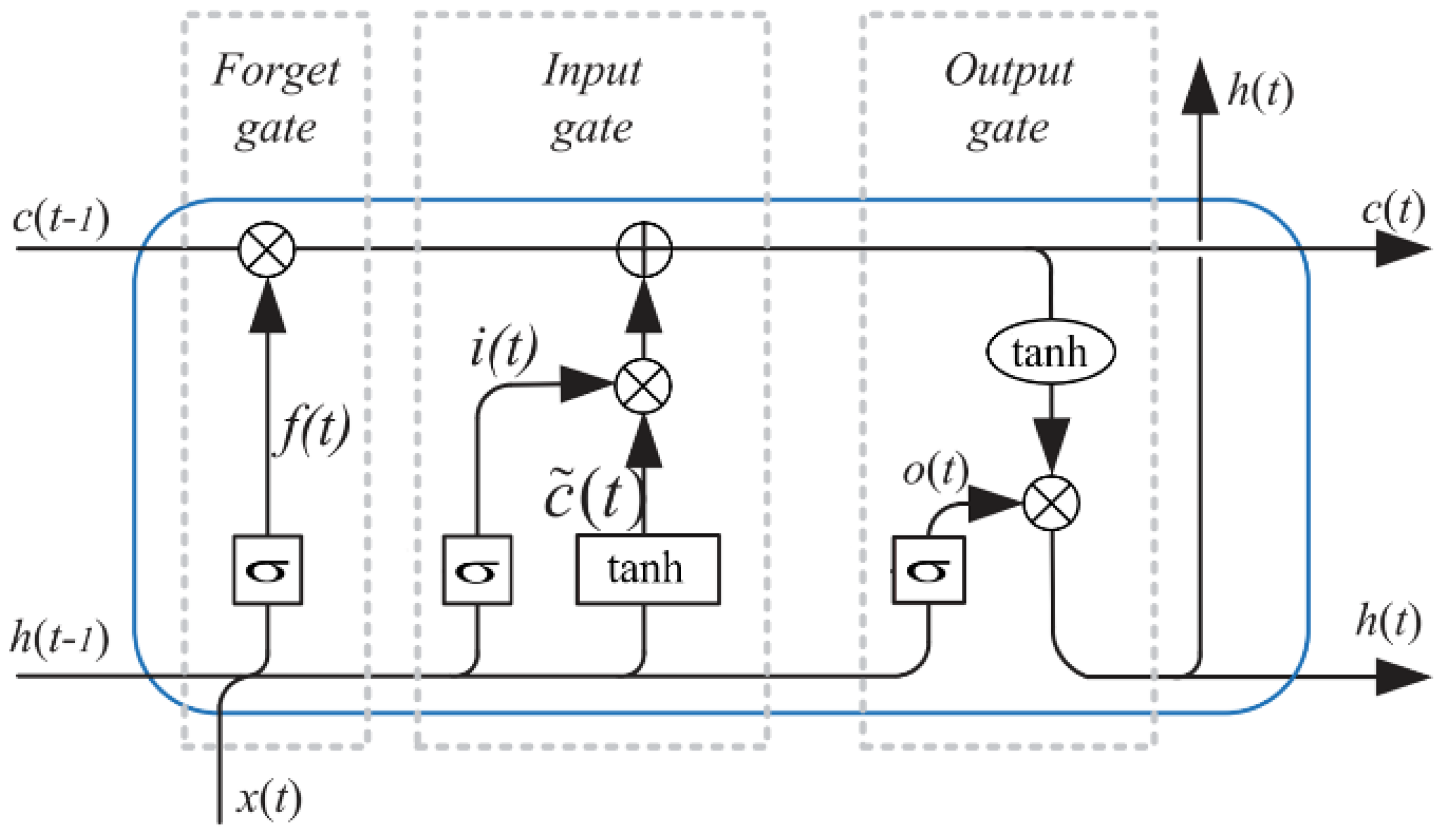
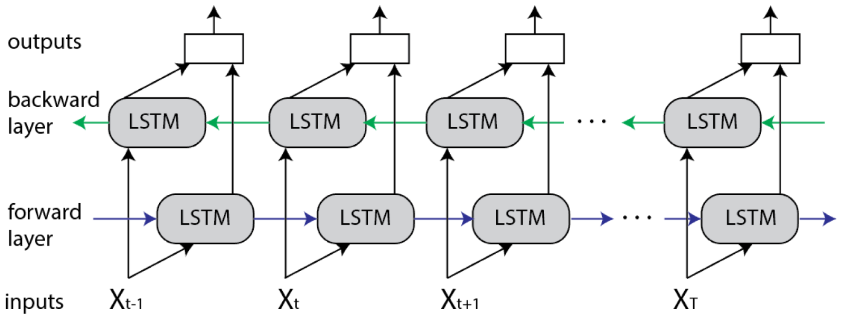
3.4. Bidirectional Long Short-Term Memory

LSTM belongs to a category of ANNs known as recurrent neural networks (RNNs), and it was developed to tackle the problem of vanishing gradients that often arises in conventional RNNs. This problem occurs when the gradients used to modify the network’s parameters become excessively small during the backpropagation process, causing difficulties in learning long-term dependencies. To overcome this issue, LSTM incorporates specialized memory cells that can selectively remember or forget information over time by including gates in the cell. An LSTM hidden layer consists of a set of recurrently connected blocks in a chain structure, known as memory blocks. Each of them contains one or more recurrently connected memory cells and three multiplicative units, called gates, that provide continuous analogues of write, read and reset operations for the cells. The architecture of the LSTM cell is shown in Figure 2.

On the basis of the connections described in this figure, we can express the LSTM cell mathematically as follows [56]:

$$\begin{array}{c}\hfill \begin{array}{cc}\hfill f_t& =\sigma (W_{fh}{h}_{t-1}+W_{fx}{x}_t+b_f)\hfill \\ \hfill i_t& =\sigma (W_{ih}{h}_{t-1}+W_{ix}{x}_t+b_i)\hfill \\ \hfill {\tilde{c}}_t& =tanh(W_{\tilde{c}h}{h}_{t-1}+W_{\tilde{c}x}{x}_t+b_{\tilde{c}})\hfill \\ \hfill c_t& =f_t\ast c_{t-1}+i_t\ast {\tilde{c}}_t\hfill \\ \hfill o_t& =\sigma (W_{oh}{h}_{t-1}+W_{ox}{x}_t+b_o)\hfill \\ \hfill h_t& =o_t\ast tanh\left(c_t\right)\hfill \end{array}\end{array}$$

(4)

At time step t, we use the activation vectors $i_t$, $f_t$, $o_t$ and $c_t$ to represent the input, forget, output and cell state gates, respectively. We denote the weight matrix by W, and the bias matrix by b. The Sigmoid function is represented by the symbol $\sigma$, and the element-wise multiplication is denoted by “∗”. The flow of information into and out of the cell is controlled by these gates, and the cell remembers values over arbitrary time intervals. More precisely, the input gate determines which values should be updated in the memory cell, the forget gate determines which values should be discarded from the memory cell, and the output gate determines which values should be used to produce the output.

Bidirectional LSTM is a type of RNN that differs from the standard LSTM by its ability to handle input sequences in both the forward and backward directions. This unique characteristic enables the network to effectively capture and utilize a broader range of input information.

It achieves this by adding a second set of hidden states that process the input sequence in reverse order, where one layer processes the input sequence in the forward direction, and the other processes it in the backward direction. The input sequence flows in both states, and the resulting outputs from each direction are merged to generate the final output. This means that the two states’ outputs are not connected to the inputs of the opposite direction’s states. This structure can be illustrated as a diagram unfolded over multiple time steps, such as the one shown in Figure 3. BiLSTM is primarily trainable using the same algorithms as a standard unidirectional LSTM. This is because the two types of state neurons do not interact and can be transformed into a general feedforward network. However, during the backpropagation through time (BPTT) process, additional steps are necessary since updating the input and output layers cannot be completed simultaneously. The training process for the unfolded bidirectional network is as follows: during the forward pass, the forward states and backward states are passed first, and then the output neurons are passed. During the backward pass, the output neurons are passed first, followed by the forward and backward states. Finally, after the forward and backward passes are complete, the weights are updated.

4. Deep Learning-Based Detectors

As stated in the latter, the objective of this research is to understand the collective behavior of primary users by analyzing the temporal patterns of sensing data gathered by multiple cooperative SUs. Cooperative spectrum sensing has been shown to be a successful method of enhancing the detection performance. In contrast to single-node sensing, CSS employs multiple distributed nodes to improve the reliability in a collaborative way. The fusion center gathers sensed information from each SU to make the ultimate decision. Nonetheless, since the fusion center relies on binary results, it cannot incorporate confidence information, resulting in limited decision-making capabilities. To address this limitation and achieve our objective, we propose three deep neural network-based detection algorithms for CSS.

4.1. Data Requirement and Generation

The preprocessing of the raw signals is performed as a first step. The signal matrix $X_t^s$ of samples received from the s-th SU during the t-th sensing period can be denoted as

$$X_t^s=\left[\begin{array}{cccc}{x}_t^1\left(1\right)& x_t^1\left(2\right)& \cdots & x_t^1\left(N\right)\\ x_t^2\left(1\right)& x_t^2\left(2\right)& \cdots & x_t^2\left(N\right)\\ ⋮& ⋮& \ddots & ⋮\\ x_t^M\left(1\right)& x_t^M\left(2\right)& \cdots & x_t^M\left(N\right)\end{array}\right]$$

(5)

where N is the number of samples in a period and M is the number of antennas in each SU. As discussed in the previous section, the use of ML models, such as standard CNNs, to process 2D data has certain drawbacks and limitations. One major limitation is the high computational complexity, requiring specialized hardware for training, which can lead to slower execution, longer online detection times and limited suitability for real-time applications on mobile and low-power devices. As a result, the choice of participating SU devices in cooperative detection processes is limited. To address this, we propose vectorizing multi-antenna data into a one-dimensional format, which can facilitate easier processing and analysis using machine learning models. This approach can also improve the memory efficiency by significantly reducing the memory overhead and decreasing the memory footprint compared to artificially expanding the data to higher dimensions. This memory efficiency arises from data preprocessing techniques and the model architecture. The presence of fewer parameters means that less memory is required to store the model’s weights and intermediate activations during training, resulting in lower memory usage during forward and backward passes in the training process. This advantage is particularly significant when working with limited computational resources, making it a practical choice, especially in resource-constrained environments. Additionally, the application of algorithms to one-dimensional vectors can be faster. The following expression of $R_t^s$ is obtained by vectorizing the received matrix signal $X_t^s$:

$$R_t^s=\mathrm{vec}\left(X_t^s\right)$$

(6)

We proceed to organize the input samples as labeled data by rearranging them in the following format: $(R_1^s,y_1),(R_2^s,y_1),\dots ,(R_T^s,y_T)$, where the label of the t-th data point is denoted by $y_t\in \{0,1\}$ to represent the hypotheses H${}_1$ and H${}_0$, and T represents the total number of data points (i.e., sensing periods taken into consideration).

4.2. Network Architecture Design

The fundamental concept underlying our proposed designs is the integration of an end-to-end architecture comprising a 1DCNN and LSTM network. The objective of this choice is to effectively capture both local patterns and temporal dependencies within the received signal, optimizing the extraction of informative features from the SS observations. Given the cooperative nature of spectrum sensing, where multiple SUs contribute their processed inputs to a fusion center, we propose two distinct DNN designs. The first design employs an end-to-end 1DCNN and LSTM at the SU level. This architecture ensures that each SU benefits from the comprehensive feature extraction capabilities of the 1DCNN and LSTM layers, contributing enhanced and refined information for cooperative decision making at the fusion center. In the second design, we introduce a variation by incorporating a BiLSTM in conjunction with the 1DCNN, maintaining an end-to-end framework. This choice allows the model to consider bidirectional temporal dependencies, potentially capturing more nuanced patterns in the spectrum sensing signals. When replacing the LSTM with a BiLSTM, we anticipate a modest improvement in accuracy. However, it is acknowledged that this potential enhancement comes with a trade-off: an increase in computational resource requirements, system complexity and processing time. In the context of CSS, where real-time decision making is crucial, minimizing the processing time and resource utilization is of paramount importance. By presenting both designs, we aim to thoroughly evaluate the trade-off between enhanced accuracy and the practical constraints of computational efficiency. The decision to offer two alternatives underscores our commitment to providing a nuanced understanding of the implications of each design choice. Both designs feature a fusion center utilizing MLP networks. This choice enables flexible and fast adaptive information fusion, optimizing cooperative decision making based on processed inputs from multiple SUs. MLP networks are generally fast to compute, thus reducing the processing time at the fusion center, which allows us to mitigate one of the main CSS constraints. In the third design, a distinct approach was taken by employing a 1DCNN solely at the SU level, while introducing a cooperative LSTM network at the fusion center level. The decision to utilize a 1DCNN at the SU level is rooted in its ability to effectively capture local patterns, providing a focused feature extraction process tailored to the characteristics of the individual SUs. This localized processing helps in extracting relevant information before transmitting it to the fusion center. At the fusion center level, the introduction of a cooperative LSTM serves a dual purpose. Rather than an end-to-end LSTM, the cooperative LSTM is designed to undertake two critical tasks. First, it plays a role akin to an end-to-end LSTM, capturing and understanding the temporal dependencies within the data received from the SUs. This functionality ensures that the fusion center comprehensively analyzes the sequential nature of the spectrum sensing data, considering the historical context for decision making. The second task of the cooperative LSTM at the FC involves processing the gathered output from the SUs. This distinctive feature allows the LSTM to function as a central platform, aggregating and interpreting information from multiple SUs, thereby promoting cooperative decision making.

With the aim to address potential overfitting issues, all proposed models have been equipped with effective L2 regularization techniques. We have applied L2 regularization to both the weights of the layers and the output of the layers. L2 regularization helps to control the magnitude of the models’ parameters, preventing them from becoming overly large during training and reducing the risk of overfitting. Additionally, we have included dropout layers to introduce stochasticity during training, forcing the models to learn robust features and preventing them from relying too heavily on specific patterns present in the training data. These measures collectively contribute to enhancing the generalization capabilities of the models and mitigating overfitting concerns.

Considering the critical importance of computational efficiency in cooperative spectrum sensing, the proposed models underwent an optimization process. The numbers of parameters and hyper-parameters were systematically tuned to strike a balance between performance and computational resource requirements. Through extensive simulations, a thorough exploration of the models’ sensitivity to different parameter configurations was conducted. This optimization process aimed at achieving a model that not only excels in terms of accuracy but is also practical in real-world scenarios, where computational resources are often limited. The obtained results, particularly in terms of the detection time, suggest that the computational costs associated with the models are relatively modest.

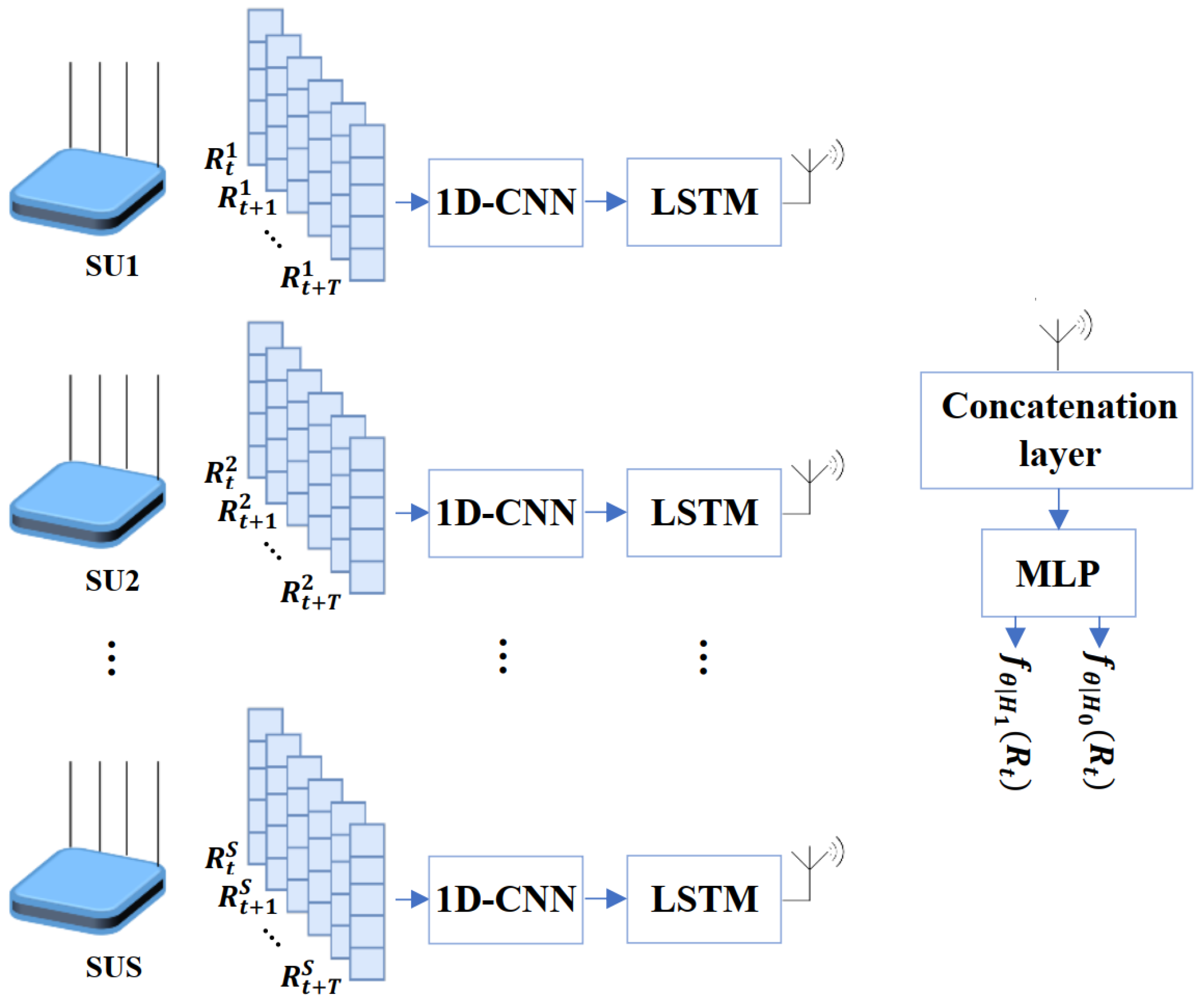
4.2.1. Hierarchical LSTM with 1DCNN

The proposed DNN model consists of a 1DCNN network at the SU level and an LSTM classifier at the fusion center. In Figure 4, a 1DCNN is shown, which consists of two convolutional blocks at the SU level. Each block includes a one-dimensional convolutional (Conv1D) layer and a rectified linear unit (ReLU) activation function. These blocks are then followed by a max pooling layer and a fully connected (FC) layer. At the fusion center level, there is a concatenation layer, an LSTM layer and a classifier network, respectively.

As is known, the 1DCNN is well suited for the extraction of local features from sequential data [55]. Employing a two-layer 1DCNN could obtain sufficient local features when tackling the SS problem, especially in low-SNR environments [32]. To leverage this capability, our proposed model includes two convolutional neural blocks to extract local patterns from the vectorized input signal. We also employ ReLU activation functions to enhance the nonlinear relationships between layers, which is essential in handling complex time series data. Additionally, we use max pooling layers to reduce the dimensionality of the resulting features and mitigate overfitting. The FC layer maps an input feature to a lower-dimensional vector. The output from the fully connected layer is then flattened and used as the feature representation for each SU. In our proposed approach, we consider the transmission of the feature representation obtained from the SU level to the fusion center. The feature representation is transmitted from the SUs to the fusion center through their respective transmitting antennas. Transmitting calculated features instead of raw data yields key benefits such as reduced dimensionality, data compression and reduced redundancy. This approach optimizes bandwidth utilization while preserving data integrity and privacy. Indeed, in this specific context, when transmitting a feature vector of a fixed size containing 256 points, even without the utilization of network optimization strategies, there is typically no necessity for high bandwidth allocation in the control channel. However, due to factors such as distortion or errors during the transmission process, the transmitted data may experience errors or corruption. To model this behavior, we incorporate a bit error rate that reflects the probability of a bit being received incorrectly at the fusion center, aiming to emulate the impact of transmission errors on the received feature representation at the fusion center. This allows us to assess the robustness and performance of our proposed model in scenarios where the transmitted data may be affected by errors.

As previously mentioned, while 1DCNNs excel at extracting local features, they often struggle to capture long-term temporal connections in the input data. To address this limitation, we incorporate an LSTM layer after concatenating the feature representations from all SUs at the fusion center. This enables us to efficiently capture the hidden connections among the extracted features by taking into account the timing regularity of the input data. By using an LSTM in the fusion center, we can also extract temporal features from the sensing data of the group level over multiple sensing periods. Thus, the cooperative LSTM models the SU-level temporal features of all cooperative SUs to learn the group-level PU activity pattern. Finally, to obtain the classification result, the LSTM layer is followed by the FC layer and Softmax layer.

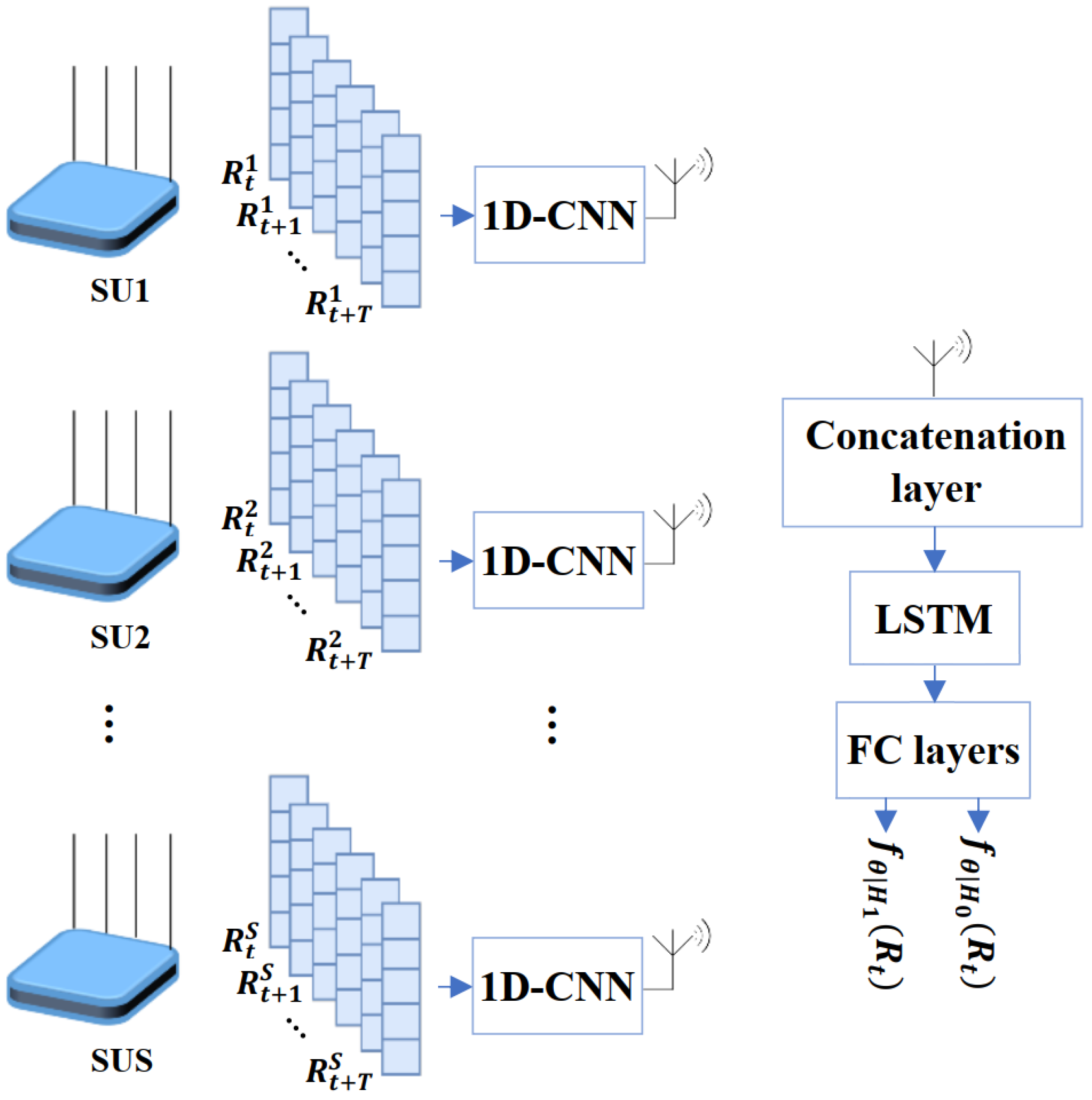
4.2.2. Hierarchical MLP with 1DCNN-LSTM

This DNN model is built with a hierarchical multilayer perceptron network-based CSS method. It incorporates an end-to-end one-dimensional convolutional neural network long short-term memory (1DCNN-LSTM) at the SU level. The complete network architecture, which includes the 1DCNN-LSTM-MLP structure, is illustrated in Figure 5.

The vectorized sequence of raw samples obtained from antennas is first sequentially used as input in the 1DCNN module, which comprises two convolutional blocks as in the previous deep neural network model. A max pooling layer is then employed to extract the most noticeable and prominent features from the resulting feature map. The resulting feature map is flattened before it is subjected to the LSTM layer to capture the long-term temporal connections of the input. Therefore, it learns the SU-level PU activity pattern from the features extracted by the convolution operation. Substantially, the end-to-end 1DCNN-LSTM network extracts local features and global correlations from the input signal. The feature representations corresponding to a particular sensing duration for each SU are then forwarded to the fusion center, which is composed of a cooperative multilayer perceptron. By using an MLP in the fusion center, the architecture can take advantage of the speed and efficiency of MLPs for final decision making, as they are generally faster to compute than LSTMs, thus reducing the processing time at the fusion center, which allows us to mitigate one of the main CSS constraints. The proposed MLP architecture employs ReLU as an activation function for the hidden layer and separates the output with a dropout layer to prevent overfitting and improve the model’s generalization. Finally, the output is mapped to a 2 × 1 class score vector, which is normalized by the Softmax function to obtain the classification result.

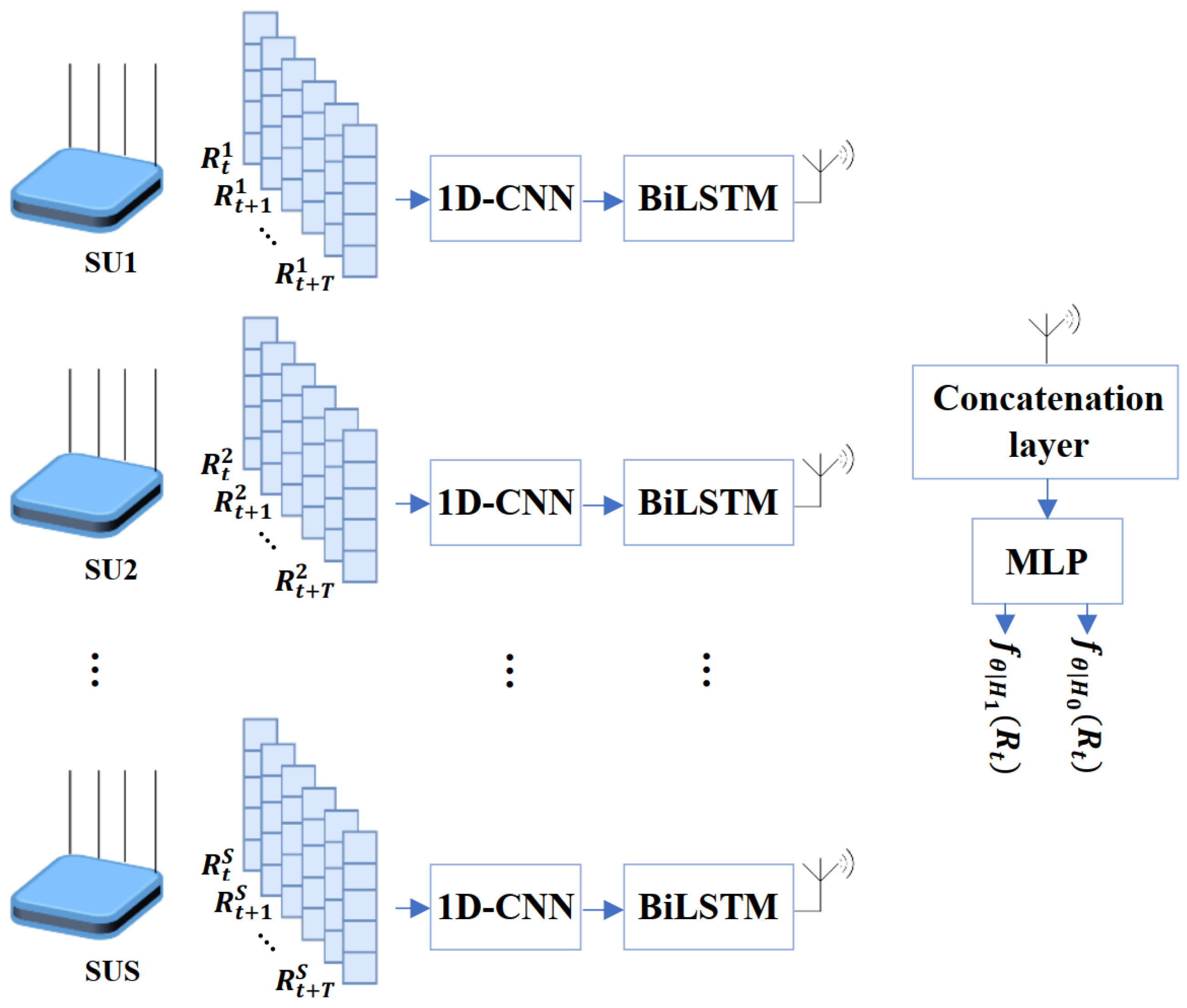
4.2.3. Hierarchical MLP with 1DCNN-BiLSTM

This DNN model is built using a CSS method based on a hierarchical multilayer perceptron network. It integrates a 1DCNN with an end-to-end bidirectional LSTM (1DCNN-BiLSTM) at the SU. The complete network architecture, which includes the 1DCNN-BiLSTM-MLP structure, is shown in Figure 6.

The current model follows the 1DCNN-LSTM-MLP architecture, except for the replacement of the LSTM model with BiLSTM in this case. We use a BiLSTM to capture long-term temporal connections between the input data and the hidden connections among the features extracted, according to the timing regularity of the input data. Unlike the standard LSTM network, which can only analyze previous data, the BiLSTM network scans the data in both directions, using both pre- and post-data simultaneously. This improves the global correlation extraction process compared to LSTM. The remaining steps of the process are identical to the previous DNN model.

4.3. Training Model

In this work, we propose an end-to-end training approach to simultaneously learn the SU-level and fusion center models using a set of training data, consisting of a sequence of vectorized signals $R_t$ with labels $y_t$. After completing the forward pass through the DNN model, a class score vector of size 2 × 1 is obtained at the output, which is normalized using the Softmax function. This is represented by Equation (7).

$$f_{\theta }\left(R_t\right)=\left[\begin{array}{c}{f}_{\theta \mid H_0}\left(R_t\right)\\ f_{\theta \mid H_1}\left(R_t\right)\end{array}\right]$$

(7)

with

$$f_{\theta \mid H_0}\left(R_t\right)+f_{\theta \mid H_1}\left(R_t\right)=1$$

(8)

where $\theta$ and $f_{\theta }(·)$ are the model’s parameters and expression, respectively. This output reflects the probabilities of the hypotheses. $f_{\theta \mid H_i}\left(R_t\right)$ is the corresponding expression of H${}_i$ (i.e., the class score of H${}_i$). As is known in supervised learning, training a neural network involves maximizing the likelihood. The goal function of the proposed DNN is based on likelihood maximization, which can be found in Equation (9).

$$L\left(\theta \right)=\prod _{t=1}^T{f}_{\theta \mid H_0}{\left(R_t\right)}^{\mathbb{1}(y_t=0)}·{(1-f_{\theta \mid H_1}\left(R_t\right))}^{\mathbb{1}(y_t=1)}$$

(9)

where $\mathbb{1}(·)$ is the indicator function. Since the cross-entropy between the training data and the model’s distribution is equivalent to the negative log-likelihood of the data under the model, the neural network loss function $J\left(\theta \right)$ can be obtained by taking the logarithm of the likelihood and normalizing it with the training set size. It is defined in Equation (10).

$$\begin{array}{c}\hfill J\left(\theta \right)=-\frac{1}{T}\sum _{t=1}^T(\mathbb{1}(y_t=0)log{f}_{\theta \mid H_0}\left(R_t\right)\\ \hfill +\mathbb{1}(y_t=1)log(1-f_{\theta \mid H_1}\left(R_t\right)))\end{array}$$

(10)

Therefore, the maximum likelihood can be reached by seeking the network parameters that minimize the loss function as

$${\theta }^{*}=arg\underset{\theta }{min}J\left(\theta \right)$$

(11)

The loss function is differentiable and, therefore, $\theta$ is updated gradually via backpropagation until the optimal parameter ${\theta }^{*}$ by conducting gradient descent on the loss function. There are several optimization algorithms commonly used to perform this adaptation: stochastic gradient descent (SGD), momentum, Adagrad, root mean square propagation (RMSprop), adaptive moment estimation (Adam), Adadelta, Nadam and limited-memory Broyden–Fletcher–Goldfarb–Shanno (L-BFGS). The choice of optimizer depends on factors such as the specific characteristics of the data, the architecture of the neural network and the computational resources. We adopt the Adam method to calculate the optimal parameters that minimize the loss function and improve the accuracy of the network. It is a powerful stochastic optimization algorithm that requires only first-order gradients, uses an adaptive learning rate, gives overall good performance and uses a moderate amount of memory.

5. Simulation Results and Discussion

In this section, the detection performance and online detection time of the proposed CSS methods, which are based on a DNN model, are evaluated. To verify the effectiveness of the proposed approach, it is compared with three benchmark methods. The comparison is conducted to assess the performance of the proposed method in terms of the detection accuracy and efficiency of online detection.

5.1. Simulation Environment

In order to evaluate the performance of our proposed system, we conducted simulations with various parameter settings. In particular, we considered a sensing period length of N samples, S SU devices and M antennas in each SU device. We assumed that the PU signal was an independent and identically distributed (i.i.d.) Gaussian random vector with zero mean and signal variance ${\sigma }_x^2$.

• For the PU-SU channel models, we assumed

• noise signals $w_s^m$ as i.i.d. Gaussian random vectors with zero mean and variance ${\sigma }_{w_s^m}^2$ that add up the PU signal at the SU receivers;
• gains $h_s^m$ following a Rayleigh distribution with parameter ${\sigma }_h$.

Here, $s\in [1,\dots ,S]$ identifies each specific SU and $m\in [1,\dots ,M]$ identifies a specific antenna in the SU.

The signal generation process begins by converting the desired SNR from decibels to a linear scale and by generating, if it is in the active state, the transmitted signal of the PU for a specific sensing period. For each antenna of each SU, the transmitted PU signal will be scaled using the specific gain of the related channel $h_s^m$. The resulting power of the received signal, $R{P}_s^m$, is then computed using the squared magnitude of each scaled signal sample. The power of the noise is determined based on the desired SNR, and Gaussian noise with the related variance ${\sigma }_{w_s^m}^2$ is generated. The scaled noise is finally added to the scaled signal, resulting in a new signal that reflects fading and the specified SNR. Moreover, we assumed the channels to be time-invariant during each sensing period.

To model the bidirectional transmissions between the SUs and the fusion center, we assumed channels that exhibit a fixed BER value with no automatic repeat request (ARQ) or forward error correction (FEC) mechanisms at the data link layer.

The environment parameters used in the simulations are presented in

Table 1. Environment parameters.

Symbol	Description	Value
N	Number of samples in a sensing period	64
S	Number of cooperating SUs	4
M	Number of antennas on each SU	4
$x\left[n\right]$	PU samples	Gaussian random variables
${\mu }_x$	PU sample mean	0
${\sigma }_x^2$	PU sample variance	1
$h_s^m$	Path gain at antenna m of SU s	Rayleigh random variable
${\sigma }_h$	Scale parameter of the Rayleigh distribution	$\frac{\sqrt{2}}{2}$
$w_s^m\left[n\right]$	Noise samples at antenna m of SU s	Gaussian random variables
${\mu }_w$	Noise sample mean	0
${\sigma }_{w_s^m}^2$	Noise sample variance	Evaluated according to desired SNR and current $R{P}_s^m$
SNR	default SNR at SU	$-14$ dB
BER	Bit error rate for service messages	${10}^{-4}$

.

5.2. Model Hyper-Parameters and Training Conditions

We conducted a thorough analysis, running the DL models on various occasions to ensure robustness and to explore potential variability in the results. Prior to reporting the results, the models were executed multiple times to identify the optimal configurations and assess the stability of their performance.

We trained our models using different filter numbers and assessed their performance on a validation set. Our decision-making process was informed by the validation performance, leading us to select configurations that yielded optimal performance without overfitting. The selection of filter numbers was influenced by various factors, including the data characteristics, task complexity, model architecture and resource constraints. Ultimately, identifying the optimal set of hyper-parameters, including the filter number, entails a combination of educated guesswork and empirical experimentation based on experience.

Table 2. Model hyper-parameters.

Parameter Settings	Parameter Description	Layer Name
CNN module	(Activation: ReLU)
Input	(256 × 1)
Kernel number and size	(40, 9)	Conv 1, 2
Pool size	2	MaxPool
LSTM module	Unit number: 64	LSTM layer 1
BiLSTM module	Unit number: 64	BiLSTM layer 1
Cooperative LSTM	Unit number: 64	CLSTM layer 1
Cooperative MLP	Unit number: 128, 64, 2	MLP layer 1, 2, 3

summarizes the model hyper-parameters used for the different proposed architectures.

During the training phase, the dataset incorporated several SNR values, and the instances were shuffled to expose the models to various SNR conditions. Specifically, we generated examples with SNR values in the set $\{-20\mathrm{dB},-19\mathrm{dB},\dots ,-1\mathrm{dB},0\mathrm{dB}\}$, which contained discrete SNR values in the range between $-20$ dB and 0 dB with a step of 1 dB. This strategy aimed to enhance the model’s adaptability to a wide spectrum of SNR scenarios, ensuring robust performance across different signal quality levels.

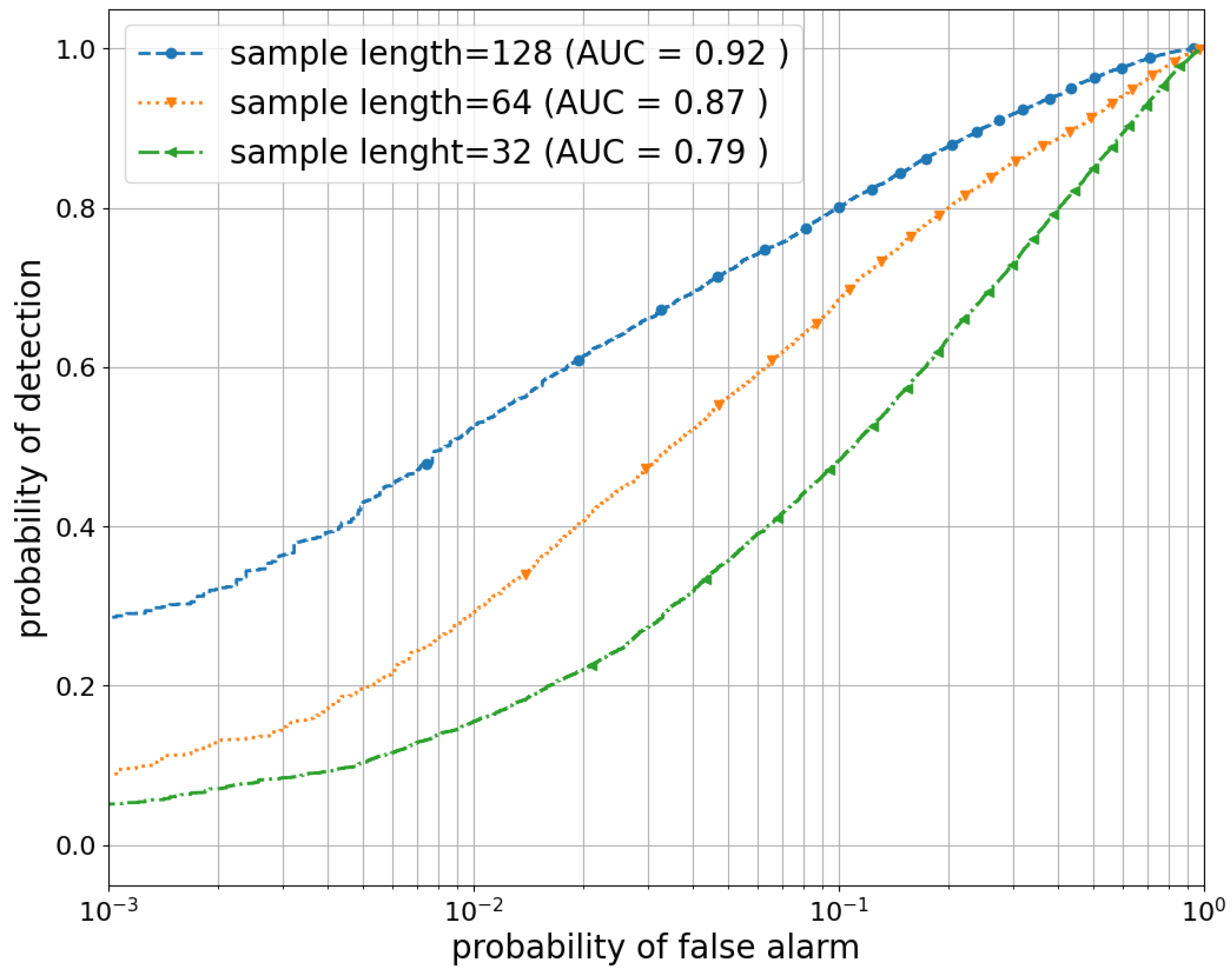
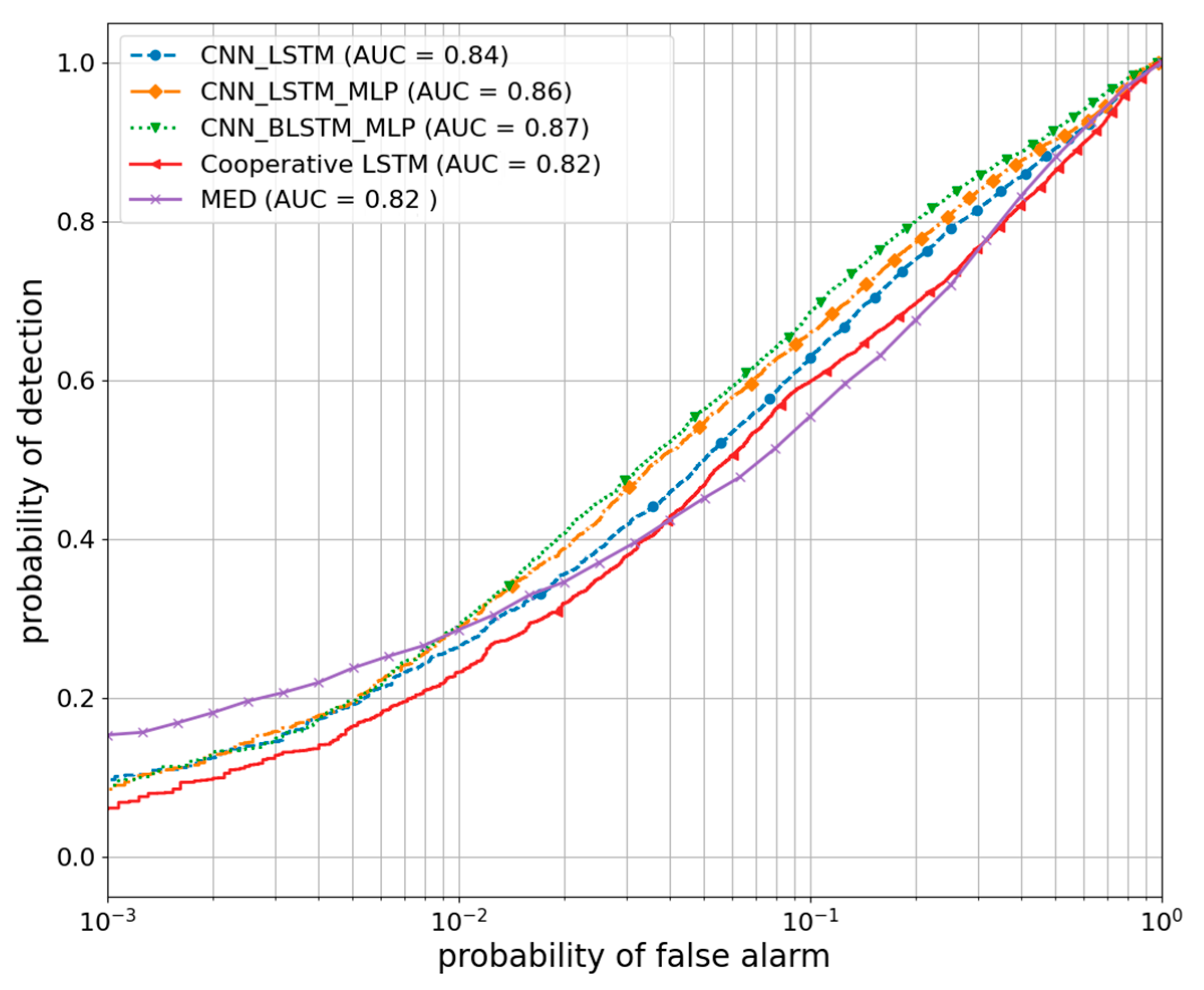
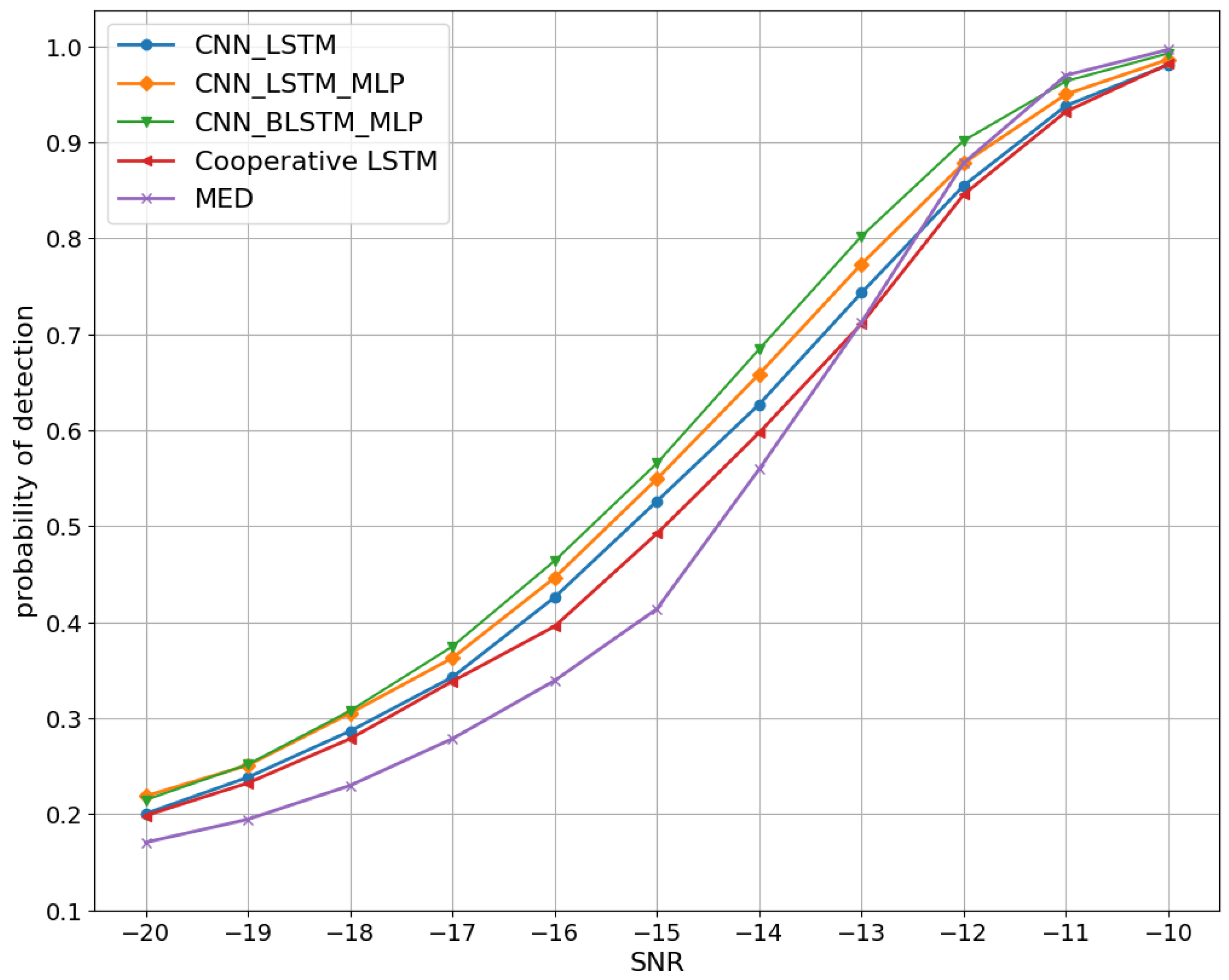
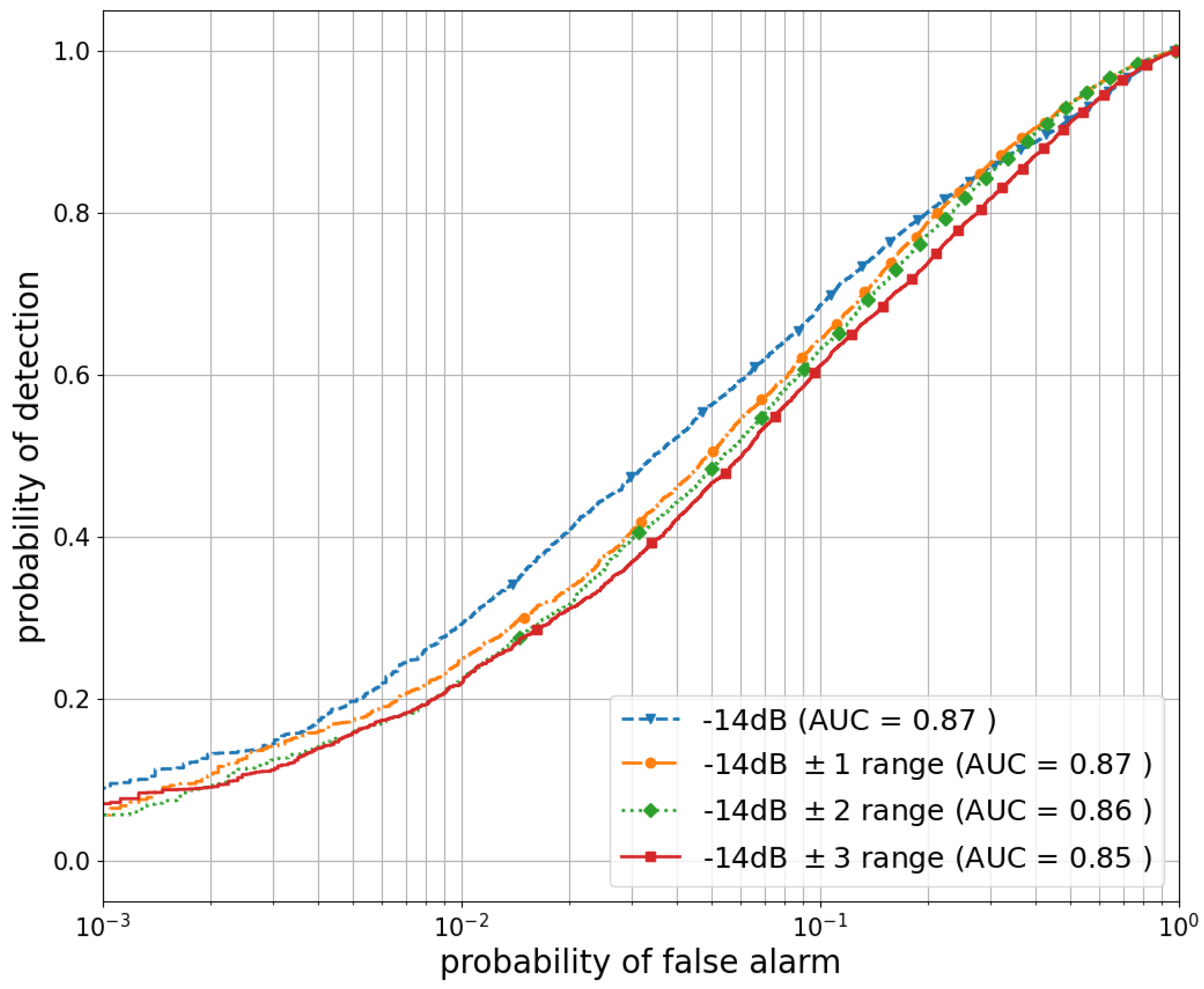
5.3. Performance Evaluation

The simulations were conducted on an NVIDIA Tesla T4 with 16 GB of GDDR6 memory and 3072 CUDA cores, with the TensorFlow framework. To demonstrate the effectiveness of our proposed cooperative spectrum detection methods based on deep neural networks, we present detailed simulation results. Our evaluation of the detection performance includes analyzing the receiver operating characteristic (ROC) curve, detection probability ($P_d$) versus signal-to-noise ratio (SNR) and online detection time. Furthermore, we compare the performance of our methods with two existing state-of-the-art methods: the maximum eigenvalue detector [24] and the hierarchical cooperative LSTM method proposed by [17].The first one was implemented as in [24], computing the sample covariance matrix starting from all the samples in a sensing period and then computing the maximum eigenvalue ${\lambda }_{max}$ of this sample covariance matrix and, finally, performing the decision according to the relation ${\lambda }_{max}>\gamma {\sigma }_w^2$, where ${\sigma }_w^2$ is the variance of all the noise samples and $\gamma$ is theoretically derived to meet the $P_{fa}$ requirement. The second one uses a hierarchical cooperative LSTM network to process the covariance matrices (CMs) generated by the sensing data of each SU through an end-to-end CNN LSTM. To ensure a fair comparison, we employ the default hyper-parameter settings for each existing model as reported in the literature.

The trained models were evaluated using separate SNR values to assess their performance under specific conditions. This approach allowed for a more focused examination of the model’s effectiveness in handling individual SNR levels, providing insights into its capability to generalize and perform well across varying signal-to-noise scenarios during testing. Therefore, while the training set aimed for a comprehensive adaptation, the test set focused on evaluating the model’s performance under specific SNR conditions. Specifically, to evaluate the ROC curves, we fixed the SNR at $-14$ dB, while, when we evaluated the results in terms of the probability of detection when varying the SNR, we considered the latter in the range from $-20$ dB to $-10$ dB with a step of 1 dB and we fixed at $0.1$ the probability of false alarms.

The ROC curve presented in Figure 7 illustrates the performance of the proposed deep neural network techniques compared to existing methods under the $-14$ dB SNR condition. It is evident that all DL-based detectors outperformed the conventional SS detector. This outcome is expected due to the ability of deep neural networks to learn intricate patterns from input signals, surpassing the capabilities of traditional statistical signal processing techniques in capturing such complexities. For instance, at a false alarm probability of $0.1$, the CNN_BLSTM_MLP detector achieves a detection probability of $69\%$, followed by the CNN_LSTM_MLP detector at $67\%$ and the CNN_LSTM and cooperative LSTM detectors at $63\%$ and $60\%$, respectively. To further assess the overall detection performance and compare the models comprehensively, we calculated the area under the curve (AUC) values. The AUC values corroborated the findings from the detection probabilities, indicating that the models employing an end-to-end 1DCNN RNN structure at the SU level demonstrated superior performance in terms of sensitivity at low $P_{fa}$ rates and overall detection capability compared to the CNN_LSTM and cooperative LSTM detectors.

Additionally, we examined the detection performance of the proposed method across various SNR levels by plotting the detection probability against the SNR curves. Figure 8 displays these curves for the proposed detectors, as well as other conventional methods, with a fixed $P_{fa}$ of $0.1$. Our focus is on showcasing the simulation results using signals with lower SNRs ranging from $-20$ dB to $-10$ dB, as models that excel at lower SNRs tend to perform better at higher SNRs as well. Despite observing some performance degradation at low SNR values, the proposed DNN methods still exhibit promising outcomes. Notably, the CNN-LSTM detector does not perform as well as the other proposed detectors that utilize an end-to-end 1DCNN RNN structure at the SU level. This disparity can be attributed to the structure of the CNN-LSTM detector. The challenge lies in efficiently integrating information by combining the outputs of the 1DCNN from all SUs before processing with a single LSTM. There is a potential loss of individual SU-specific information in this approach. On the contrary, employing separate LSTMs at each SU allows for the individual modeling and capture of SU-specific information. This enables the model to learn hierarchical representations directly from the raw signal data, which proves advantageous when the raw signal contains critical temporal patterns or spatial features crucial for SS. Furthermore, it is evident that the proposed DNN model based on bidirectional LSTM outperforms the one based on unidirectional LSTM. This superiority stems from the bidirectional LSTM’s capability to effectively capture temporal features from the signals, resulting in improved detection performance.

Moreover, it appears evident that the MED algorithm outperforms the proposed ones under low-noise conditions (actually, starting from $-12$ dB). This occurs due to its simplicity and the direct nature of its comparison algorithm. This feature makes the distinction between statistical test results and the threshold more obvious under low-noise conditions. Although MED seems to perform best under high SNR conditions, it should be noted that the DNN maintains near-perfect performance too, which is acceptable. The DNN is trained under a wide range of low SNR conditions, enabling it to efficiently extract complex patterns and features from signals, even in challenging and noisy environments typical of low SNR scenarios. The wide range of low SNR conditions in our training data, while beneficial for robust performance in challenging environments, may marginally affect the DNN’s performance at higher SNR values. Consequently, the observed superiority of our approach in low SNR environments aligns perfectly with our design objectives and meets the practical requirements of real-world applications. Importantly, the DNN also addresses the limitations of traditional approaches, such as MED, at low SNR conditions.

Ensuring high accuracy in SS is crucial in granting SUs access to the spectrum while avoiding interference with the primary user. However, this increased accuracy also leads to a longer sensing time, thereby reducing the permitted data transmission time for SUs. Therefore, it is essential to determine an optimal sensing time that maximizes the throughput for SUs while adequately protecting the PU. To evaluate the proposed methods, we compare their response times, specifically the time required to classify an example (which consists of a sensing period of 64 samples).

The computation time results for various methods are summarized in

Table 3. Computation time comparison of different methods (sensing period: 64 samples).

Method	Online Detection (ms)
CNN_LSTM	22
CNN_LSTM_MLP	22
CNN_BLSTM_MLP	23
Cooperative LSTM	25

, where the online detection time is measured in milliseconds. According to the table, it is evident that all DNN methods exhibit higher online detection times. This can be attributed to the parallelization of convolution operations using a GPU, whereas LSTM operations cannot be parallelized. Notably, the conventional SS method demonstrates the shortest online detection time since the maximum eigenvalue detector involves simpler computations compared to a DNN, which typically entails more complex operations involving forward propagation through multiple layers. However, this trade-off is offset by the superior accuracy offered by the DNN-based methods. Although the cooperative LSTM approach utilizes a $15\times 15$ input shape, which is still lower than our vectorized input, it exhibits the highest online detection time due to the two-dimensional CNN architecture and computational complexity discussed earlier. In comparison to other proposed methods, the bidirectional LSTM-based method incurs the longest online detection time among the proposed approaches, but it only requires an additional millisecond to process a single piece of input data. Nevertheless, it delivers the best performance across all SNR conditions. Consequently, we can conclude that the methods based on bidirectional LSTM present the most favorable compromise.

Furthermore, we examine the influence of different sample lengths on the detection performance. We specifically set the sample length, denoted as N, to three different values: 32, 64 and 128. Figure 9 illustrates the receiver operating characteristic curves of the proposed bidirectional LSTM-based method for these various sample lengths. The graph clearly demonstrates that a larger sample length leads to a higher probability of detection. This is attributed to the fact that longer samples contain a greater amount of correlation and pattern information, allowing for the more accurate extraction of temporal features from the received signal data. However, it is important to note that longer sample lengths introduce increased computational complexity and latency, which can be problematic for real-time applications that require swift response times. Therefore, when contemplating the utilization of larger sample lengths, it is essential to carefully consider the trade-off between the potential benefits of enhanced accuracy and these associated drawbacks.

In a CSS systems, SU devices often operate at different SNR levels. This variation in SNR can occur due to several factors, including differences in the distance from the PU transmitter, varying channel conditions, varying interference levels and different transmission power levels. Considering this inherent variability in the SNR among SU devices is important for the realistic simulation and evaluation of CSS systems. It enables a more accurate assessment of the system’s performance and its ability to adapt to and operate in the diverse SNR conditions commonly encountered in real-world scenarios. To simulate this scenario, a specific approach was employed. To each SU device, we assigned a mean SNR value of $-14$ dB; the actual SNR was obtained by adding random values chosen from a uniform distribution with different ranges. Three separate simulations were conducted using the bidirectional LSTM models. In each simulation, the added values were uniformly selected from the ranges $[-1,1]$ dB, $[-2,2]$ dB and $[-3,3]$ dB, respectively. The results obtained from the aforementioned scenario were then compared to the previous case, as described earlier, where all SU devices were assumed to share the same SNR value.

Figure 10 illustrates the results according to the specific scenario described above. The analysis of the presented scenario revealed that the model’s performance remained remarkably close to the scenario where all SU devices employed the same SNR value. This observation demonstrates the generalization capacity of our model, as it successfully adapts to the diverse SNR conditions encountered in practical deployments. However, it is important to note that as the range of SNR values for the SU devices was expanded, a decline in performance became evident. This observation suggests that increasing the range beyond a certain threshold negatively impacts the model’s ability to accurately detect signals.

6. Conclusions and Future Work

In our study, we presented a CSS model based on a tree deep neural network architecture that combines a one-dimensional convolutional neural network (1DCNN) and a long short-term memory (LSTM) network. The purpose of this model is to learn the activity patterns of the primary user. In CSS, the collaboration of all SUs is essential in determining the PU state. Therefore, our model is designed to learn the PU activity pattern at the SU level by utilizing a vectorized input obtained from multiple antennas. By incorporating 1DCNN and LSTM layers into our model, we enable the learning of group-level PU activity patterns by capturing local features and global correlations. This integration enhances the overall detection performance. Through a comprehensive simulation analysis, we have determined that the DNN method based on bidirectional LSTM outperforms conventional methods and other proposed techniques in terms of detection performance, in scenarios involving imperfect reporting channels. This improvement can be attributed to its ability to capture substantial global correlations compared to the alternative methods. Furthermore, this approach strikes a favorable balance between detection accuracy and online detection, outperforming conventional and alternative approaches, which makes it a promising solution for CSS applications. Lastly, we observed that utilizing samples with larger lengths contributed to higher detection accuracy. This finding emphasizes the importance of considering longer sample lengths when aiming for improved performance in PU activity detection. Our study focused on evaluating the performance of the proposed model in various SNR scenarios for SU devices. The results obtained highlight the model’s ability to generalize effectively. These results underline the significant influence of the SNR range on the overall model performance.

However, the proposed approaches are affected by some limitations that could be explored in successive studies.

• The cooperative architecture is based only on centralized processing at the fusion center. In practical applications, this could lead to delays in decision making, particularly if there are difficulties in transmitting data quickly from the SUs to the fusion center. Other network topologies and/or distributed processing can be investigated.
• The current simulation involved only four secondary users and four antennas for the SU. A more complete dataset encompassing broader SU and antenna configurations would enable a more nuanced and comprehensive assessment.
• The study did not explicitly consider scenarios in which certain SUs might be sub-optimally positioned for data transmission. Factors such as SU mobility, obstacles on the communication path or SU malfunctions could be modeled in a future work. Effectively addressing these real-world challenges can lead to a more authentic evaluation of the cooperative spectrum sensing system.
• Finally, situations in which cooperation fails should be addressed. A thorough understanding and effective mitigation of these cases of cooperation failure can give information about the resilience and reliability of the proposed models in dynamic wireless environments.

Regardless of these limitations, the three DNN models proposed for cooperative spectrum sensing can already have direct and important applications in various scenarios. The proposed models offer significant advantages in applications such as dynamic spectrum access, cognitive radio networks and others. In dynamic spectrum access, where the spectrum availability changes dynamically, the ability to capture temporal dependencies can ensure adaptive and efficient spectrum use. In cognitive radio networks, the proposed models can enable collaborative sensing among secondary users, improving the overall reliability and accuracy of spectrum occupancy detection. These applications extend to scenarios in which the environmental conditions, signal characteristics and interference patterns evolve over time. Overall, the proposed models align with most of the requirements of real-world applications for cooperative spectrum sensing, helping to improve spectrum utilization and decision making in dynamic wireless environments.

References

1. Atzori, L.; Iera, A.; Morabito, G. The Internet of Things: A survey. Comput. Netw. 2010, 54, 2787–2805. [Google Scholar] [CrossRef]
2. Raj, P.; Raman, A.C. Intelligent Cities: Enabling Tools and Technology; CRC Press: Boca Raton, FL, USA, 2015. [Google Scholar]
3. Bin Sahbudin, M.A.; Chaouch, C.; Scarpa, M.; Serrano, S. IoT based Song Recognition for FM Radio Station Broadcasting. In Proceedings of the 2019 7th International Conference on Information and Communication Technology (ICoICT), Kuala Lumpur, Malaysia, 24–26 July 2019; pp. 1–6. [Google Scholar] [CrossRef]
4. Aswathy, G.P.; Gopakumar, K. Sub-Nyquist Wideband Spectrum Sensing Techniques for Cognitive Radio: A Review and Proposed Techniques. AEU-Int. J. Electron. Commun. 2019, 104, 44–57. [Google Scholar] [CrossRef]
5. Mitola, J.; Maguire, G. Cognitive radio: Making software radios more personal. IEEE Pers. Commun. 1999, 6, 13–18. [Google Scholar] [CrossRef]
6. Yucek, T.; Arslan, H. A survey of spectrum sensing algorithms for cognitive radio applications. IEEE Commun. Surv. Tutorials 2009, 11, 116–130. [Google Scholar] [CrossRef]
7. Serrano, S.; Scarpa, M. A Petri Net Model for Cognitive Radio Internet of Things Networks Exploiting GSM Bands. Future Internet 2023, 15, 115. [Google Scholar] [CrossRef]
8. Nasser, A.; Al Haj Hassan, H.; Abou Chaaya, J.; Mansour, A.; Yao, K.C. Spectrum Sensing for Cognitive Radio: Recent Advances and Future Challenge. Sensors 2021, 21, 2408. [Google Scholar] [CrossRef]
9. Patil, A.; Iyer, S.; Lopez, O.L.; Pandya, R.J.; Pai, K.; Kalla, A.; Kallimani, R. A Comprehensive Survey on Spectrum Sharing Techniques for 5G/B5G Intelligent Wireless Networks: Opportunities, Challenges and Future Research Directions. arXiv 2022, arXiv:2211.08956. [Google Scholar] [CrossRef]
10. Hu, X.L.; Ho, P.H.; Peng, L. Fundamental Limitations in Energy Detection for Spectrum Sensing. J. Sens. Actuator Netw. 2018, 7, 25. [Google Scholar] [CrossRef]
11. Serrano, S.; Scarpa, M.; Maali, A.; Soulmani, A.; Boumaaz, N. Random sampling for effective spectrum sensing in cognitive radio time slotted environment. Phys. Commun. 2021, 49, 101482. [Google Scholar] [CrossRef]
12. Barrak, S.E.; Lyhyaoui, A.; Gonnouni, A.E.; Puliafito, A.; Serrano, S. Application of MVDR and MUSIC Spectrum Sensing Techniques with Implementation of Node’s Prototype for Cognitive Radio Ad-Hoc Networks. In Proceedings of the 2017 International Conference on Smart Digital Environment, New York, NY, USA, 21–23 July 2017; pp. 101–106. [Google Scholar] [CrossRef]
13. Coluccia, A.; Fascista, A.; Ricci, G. Spectrum sensing by higher-order SVM-based detection. In Proceedings of the 2019 27th European Signal Processing Conference (EUSIPCO), A Coruna, Spain, 2–6 September 2019; pp. 1–5. [Google Scholar] [CrossRef]
14. Saber, M.; El Rharras, A.; Saadane, R.; Kharraz, A.H.; Chehri, A. An Optimized Spectrum Sensing Implementation Based on SVM, KNN and TREE Algorithms. In Proceedings of the 2019 15th International Conference on Signal-Image Technology & Internet-Based Systems (SITIS), Sorrento, Italy, 26–29 November 2019; pp. 383–389. [Google Scholar] [CrossRef]
15. Chen, W.; Wu, H.; Ren, S. CM-LSTM Based Spectrum Sensing. Sensors 2022, 22, 2286. [Google Scholar] [CrossRef]
16. Janu, D.; Singh, K.; Kumar, S. Machine learning for cooperative spectrum sensing and sharing: A survey. Trans. Emerg. Telecommun. Technol. 2022, 33, e4352. [Google Scholar] [CrossRef]
17. Janu, D.; Singh, K.; Kumar, S.; Mandia, S. Hierarchical Cooperative LSTM-Based Spectrum Sensing. IEEE Commun. Lett. 2023, 27, 866–870. [Google Scholar] [CrossRef]
18. Sarala, B.; Rukmani Devi, S.; Sheela, J.J.J. Spectrum energy detection in cognitive radio networks based on a novel adaptive threshold energy detection method. Comput. Commun. 2020, 152, 1–7. [Google Scholar] [CrossRef]
19. Kumar, A.; NandhaKumar, P. OFDM system with cyclostationary feature detection spectrum sensing. ICT Express 2019, 5, 21–25. [Google Scholar] [CrossRef]
20. Brito, A.; Sebastião, P.; Velez, F.J. Hybrid Matched Filter Detection Spectrum Sensing. IEEE Access 2021, 9, 165504–165516. [Google Scholar] [CrossRef]
21. Awin, F.; Abdel-Raheem, E.; Tepe, K. Blind Spectrum Sensing Approaches for Interweaved Cognitive Radio System: A Tutorial and Short Course. IEEE Commun. Surv. Tutor. 2018, 21, 238–259. [Google Scholar] [CrossRef]
22. Semlali, H.; Boumaaz, N.; Soulmani, A.; Ghammaz, A.; Diouris, J.F. Energy detection approach for spectrum sensing in cognitive radio systems with the use of random sampling. Wirel. Pers. Commun. 2014, 79, 1053–1061. [Google Scholar] [CrossRef]
23. Gao, R.; Qi, P.; Zhang, Z. Performance analysis of spectrum sensing schemes based on energy detector in generalized Gaussian noise. Signal Process. 2021, 181, 107893. [Google Scholar] [CrossRef]
24. Zeng, Y.; Koh, C.L.; Liang, Y.C. Maximum Eigenvalue Detection: Theory and Application. In Proceedings of the 2008 IEEE International Conference on Communications, Beijing, China, 19–23 May 2008; pp. 4160–4164. [Google Scholar] [CrossRef]
25. Kumar, A.; Khan, A.S.; Modanwal, N.; Saha, S. Experimental studies on energy and eigenvalue based Spectrum sensing algorithms using USRP devices in OFDM systems. Radio Sci. 2020, 55, 1–11. [Google Scholar] [CrossRef]
26. Tan, P.N.; Steinbach, M.; Kumar, V. Introduction to Data Mining; Pearson Education: Bangalore, India, 2016. [Google Scholar]
27. Sahbudin, M.A.B.; Scarpa, M.; Serrano, S. MongoDB Clustering using K-means for Real-Time Song Recognition. In Proceedings of the 2019 International Conference on Computing, Networking and Communications (ICNC), Honolulu, HI, USA, 18–21 February 2019; pp. 350–354. [Google Scholar] [CrossRef]
28. Wang, Y.; Zhang, Y.; Wan, P.; Zhang, S.; Yang, J. A spectrum sensing method based on empirical mode decomposition and k-means clustering algorithm. Wirel. Commun. Mob. Comput. 2018, 2018, 6104502. [Google Scholar] [CrossRef]
29. Lei, K.j.; Tan, Y.h.; Yang, X.; Wang, H.r. A K-means clustering based blind multiband spectrum sensing algorithm for cognitive radio. J. Cent. South Univ. 2018, 25, 2451–2461. [Google Scholar] [CrossRef]
30. LeCun, Y.; Bengio, Y.; Hinton, G. Deep learning. Nature 2015, 521, 436–444. [Google Scholar] [CrossRef] [PubMed]
31. Schmidhuber, J. Deep learning in neural networks: An overview. Neural Netw. 2015, 61, 85–117. [Google Scholar] [CrossRef] [PubMed]
32. Peng, Q.; Gilman, A.; Vasconcelos, N.; Cosman, P.C.; Milstein, L.B. Robust Deep Sensing Through Transfer Learning in Cognitive Radio. IEEE Wirel. Commun. Lett. 2020, 9, 38–41. [Google Scholar] [CrossRef]
33. Zheng, S.; Chen, S.; Qi, P.; Zhou, H.; Yang, X. Spectrum sensing based on deep learning classification for cognitive radios. China Commun. 2020, 17, 138–148. [Google Scholar] [CrossRef]
34. Gao, J.; Yi, X.; Zhong, C.; Chen, X.; Zhang, Z. Deep Learning for Spectrum Sensing. IEEE Wirel. Commun. Lett. 2019, 8, 1727–1730. [Google Scholar] [CrossRef]
35. Yang, K.; Huang, Z.; Wang, X.; Li, X. A Blind Spectrum Sensing Method Based on Deep Learning. Sensors 2019, 19, 2270. [Google Scholar] [CrossRef]
36. Wasilewska, M.; Bogucka, H.; Kliks, A. Federated Learning for 5G Radio Spectrum Sensing. Sensors 2021, 22, 198. [Google Scholar] [CrossRef]
37. Tan, Y.; Jing, X. Cooperative Spectrum Sensing Based on Convolutional Neural Networks. Appl. Sci. 2021, 11, 4440. [Google Scholar] [CrossRef]
38. Soni, B.; Patel, D.K.; López-Benítez, M. Long Short-Term Memory Based Spectrum Sensing Scheme for Cognitive Radio Using Primary Activity Statistics. IEEE Access 2020, 8, 97437–97451. [Google Scholar] [CrossRef]
39. Xu, M.; Yin, Z.; Zhao, Y.; Wu, Z. Cooperative Spectrum Sensing Based on Multi-Features Combination Network in Cognitive Radio Network. Entropy 2022, 24, 129. [Google Scholar] [CrossRef] [PubMed]
40. Xie, J.; Fang, J.; Liu, C.; Li, X. Deep Learning-Based Spectrum Sensing in Cognitive Radio: A CNN-LSTM Approach. IEEE Commun. Lett. 2020, 24, 2196–2200. [Google Scholar] [CrossRef]
41. Hochreiter, S.; Schmidhuber, J. Long Short-Term Memory. Neural Comput. 1997, 9, 1735–1780. [Google Scholar] [CrossRef] [PubMed]
42. Xiao, Z.; Xu, X.; Xing, H.; Luo, S.; Dai, P.; Zhan, D. RTFN: A robust temporal feature network for time series classification. Inf. Sci. 2021, 571, 65–86. [Google Scholar] [CrossRef]
43. Xing, H.; Qin, H.; Luo, S.; Dai, P.; Xu, L.; Cheng, X. Spectrum sensing in cognitive radio: A deep learning based model. Trans. Emerg. Telecommun. Technol. 2022, 33, e4388. [Google Scholar] [CrossRef]
44. Grasso, C.; Raftopoulos, R.; Schembra, G.; Serrano, S. H-HOME: A learning framework of federated FANETs to provide edge computing to future delay-constrained IoT systems. Comput. Netw. 2022, 219, 109449. [Google Scholar] [CrossRef]
45. Yang, Q.; Liu, Y.; Chen, T.; Tong, Y. Federated Machine Learning: Concept and Applications. ACM Trans. Intell. Syst. Technol. 2019, 10, 1–19. [Google Scholar] [CrossRef]
46. Chen, Z.; Xu, Y.Q.; Wang, H.; Guo, D. Federated Learning-Based Cooperative Spectrum Sensing in Cognitive Radio. IEEE Commun. Lett. 2022, 26, 330–334. [Google Scholar] [CrossRef]
47. Zhu, R.; Li, M.; Liu, H.; Liu, L.; Ma, M. Federated Deep Reinforcement Learning-Based Spectrum Access Algorithm With Warranty Contract in Intelligent Transportation Systems. IEEE Trans. Intell. Transp. Syst. 2023, 24, 1178–1190. [Google Scholar] [CrossRef]
48. Du, K.L.; Leung, C.S.; Mow, W.H.; Swamy, M.N.S. Perceptron: Learning, Generalization, Model Selection, Fault Tolerance, and Role in the Deep Learning Era. Mathematics 2022, 10, 4730. [Google Scholar] [CrossRef]
49. Wang, Y.; Li, Y.; Song, Y.; Rong, X. The Influence of the Activation Function in a Convolution Neural Network Model of Facial Expression Recognition. Appl. Sci. 2020, 10, 1897. [Google Scholar] [CrossRef]
50. Keskar, N.S.; Socher, R. Improving Generalization Performance by Switching from Adam to SGD. arXiv 2017, arXiv:1712.07628. [Google Scholar] [CrossRef]
51. Duchi, J.; Hazan, E.; Singer, Y. Adaptive Subgradient Methods for Online Learning and Stochastic Optimization. J. Mach. Learn. Res. 2011, 12, 2121–2159. [Google Scholar]
52. Reddi, S.J.; Kale, S.; Kumar, S. On the Convergence of Adam and Beyond. arXiv 2019, arXiv:1904.09237. [Google Scholar]
53. Liu, L.; Jiang, H.; He, P.; Chen, W.; Liu, X.; Gao, J.; Han, J. On the Variance of the Adaptive Learning Rate and Beyond. arXiv 2021, arXiv:1908.03265. [Google Scholar]
54. Tavares, C.H.A.; Marinello, J.C.; Proenca Jr, M.L.; Abrao, T. Machine learning-based models for spectrum sensing in cooperative radio networks. IET Commun. 2020, 14, 3102–3109. [Google Scholar] [CrossRef]
55. Kiranyaz, S.; Avci, O.; Abdeljaber, O.; Ince, T.; Gabbouj, M.; Inman, D.J. 1D convolutional neural networks and applications: A survey. Mech. Syst. Signal Process. 2021, 151, 107398. [Google Scholar] [CrossRef]
56. Yu, Y.; Si, X.; Hu, C.; Zhang, J. A review of recurrent neural networks: LSTM cells and network architectures. Neural Comput. 2019, 31, 1235–1270. [Google Scholar] [CrossRef]
Figure 1. The 1DCNN architecture.
Futureinternet 16 00014 g001
Figure 2. LSTM cell architecture.
Futureinternet 16 00014 g002
Figure 3. BiLSTM architecture.
Futureinternet 16 00014 g003
Figure 4. Proposed architecture 1: hierarchical LSTM with 1DCNN (CNN_LSTM).
Futureinternet 16 00014 g004
Figure 5. Proposed architecture 2: hierarchical MLP with 1DCNN-LSTM (CNN_LSTM_MLP).
Futureinternet 16 00014 g005
Figure 6. Proposed architecture 3: hierarchical MLP with 1DCNN-BiLSTM (CNN_BLSTM_MLP).
Futureinternet 16 00014 g006
Figure 7. ROC curves under 14 dB SNR condition.
Futureinternet 16 00014 g007
Figure 8. Pd-SNR curves with a fixed P f a of 0.1 .
Futureinternet 16 00014 g008
Figure 9. ROC curves of the proposed CNN_BLSTM_MLP approach with different sample lengths at −14 dB.
Futureinternet 16 00014 g009
Figure 10. Model ROC curves with varied SNR for cooperative SUs.
Futureinternet 16 00014 g010