Article

Multi-Scale Audio Spectrogram Transformer for Classroom Teaching Interaction Recognition

1
College of Information Engineering, Inner Mongolia University of Technology, Hohhot 010080, China
2
Key Laboratory of Perception Technology and Intelligent System of Inner Mongolia Autonomous Region, Hohhot 010080, China
*
Author to whom correspondence should be addressed.
Future Internet 2023, 15(2), 65; https://doi.org/10.3390/fi15020065
Submission received: 21 December 2022 / Revised: 27 January 2023 / Accepted: 30 January 2023 / Published: 2 February 2023

Abstract

:
Classroom interactivity is one of the important metrics for assessing classrooms, and identifying classroom interactivity through classroom image data is limited by the interference of complex teaching scenarios. However, audio data within the classroom are characterized by significant student–teacher interaction. This study proposes a multi-scale audio spectrogram transformer (MAST) speech scene classification algorithm and constructs a classroom interactive audio dataset to achieve interactive teacher–student recognition in the classroom teaching process. First, the original speech signal is sampled and pre-processed to generate a multi-channel spectrogram, which enhances the representation of features compared with single-channel features; Second, in order to efficiently capture the long-range global context of the audio spectrogram, the audio features are globally modeled by the multi-head self-attention mechanism of MAST, and the feature resolution is reduced during feature extraction to continuously enrich the layer-level features while reducing the model complexity; Finally, a further combination with a time-frequency enrichment module maps the final output to a class feature map, enabling accurate audio category recognition. The experimental comparison of MAST is carried out on the public environment audio dataset and the self-built classroom audio interaction datasets. Compared with the previous state-of-the-art methods on public datasets AudioSet and ESC-50, its accuracy has been improved by 3% and 5%, respectively, and the accuracy of the self-built classroom audio interaction dataset has reached 92.1%. These results demonstrate the effectiveness of MAST in the field of general audio classification and the smart classroom domain.

1. Introduction

The rapid development of deep learning has contributed to a level of intelligence in the modern education industry; with the help of artificial intelligence algorithms, teachers can be assisted in recording and analyzing classroom conditions [1,2,3]. The degree of teacher–student interaction in the classroom can be reflected in the classroom behaviors of students and teachers, such as students taking the initiative to ask questions, passively answering teachers’ questions, group discussions and so on. However, due to a large number of students and the complexity of the scene in traditional classrooms, as well as the hidden nature of teacher–student interactions, it is difficult and unstable to effectively locate students who are interacting. Because of the above issues, mining classroom audio features and using salient voice interaction data of teachers and students within the classroom helps to understand the state of the classroom and improve the effectiveness of classroom teaching and learning. A productive and active classroom is often characterized by the presence of multiple voices, such as students interacting with the teacher in question-and-answer sessions, and students interacting with each other in discussions. A classroom that bores students often has long periods of teacher lectures or even silence within it, and students’ classroom effectiveness is significantly reduced when effective interaction is lacking. Flanders’ interactive system [4] has the class recorded manually, which not only tends to lead to missing records but also consumes a lot of human resources. Therefore, combining intelligent recognition algorithms to more efficiently identify the status of classroom voice interactions helps to address the lack of automated classroom analysis tools for traditional teaching evaluation.
Sound is one of the bridges through which humans communicate information, and audio recognition algorithms enable tasks such as speech emotion analysis [5,6], environmental audio classification [7,8], etc. Earlier methods extracted low-level descriptors such as Mel frequency, spectral coefficients, spectral centroids and spectral flatness, and combined them with methods such as support vector machines (SVM) and k-nearest neighbor rules (KNN) to complete sound classification [9,10,11]. Additionally, with the improvement of computer performance, Convolutional Neural Network (CNN) based feature extraction methods such as AlexNet [12], VGGNet [13] and ResNet [14] have been proposed to improve the accuracy of image recognition and feature extraction. The subsequent CNN is widely used to learn representations from audio spectrograms for end-to-end modeling [15,16].
From the perspective of algorithm, although the above methods have been applied in different fields, the methods based on convolutional neural networks have a certain degree of limitation and lack modeling of temporal features in the audio recognition process. Following this, researchers proposed a recognition method based on convolutional recurrent neural networks (CRNN) and introduced an attention mechanism [17,18,19,20,21,22,23]. Audio features are extracted by a CNN, which is used as input to a recurrent neural network (RNN) [24], and the attention mechanism finishes the weighting of the features. This not only enhances the temporal modeling of the spectrograms, but CRNN is also able to attend to the important feature maps in the spectrograms. However, due to the nature of convolutional computing, the process of feature extraction only focuses on local information and lacks global modeling of spectral features. In [25], the Audio Spectrograph Transformer (AST) was introduced, which is the first non-convolutional, purely attention-based audio classification model that captures the global context even at the lowest level. In terms of performance, CRNN methods lack global modeling of audio and are limited in terms of recognition accuracy; the Transformer-based audio classification method is computationally intensive and has poor applicability in limited device scenarios.
In application, human emotions play an important role in classroom learning. Based on AffectNet [26], the largest database of facial expressions, values and arousals in the wild, excellent visual analysis methods for facial emotions have emerged. Emotion-GCN [27] uses graph convolutional networks (GCNs) to recognize facial expressions in the wild. EmoAffectNet [28] consists of a robust pre-trained backbone model and a temporal subsystem to many video frames with good generalization by modeling the temporal dependence of the frames. These methods have been transferred and used to identify student behavior and academic emotions in the classroom [29,30,31,32]. Among them, Multi-task EfficientNet-B2 [33] identifies emotions and engagement in online learning and is more innovative. Existing approaches to intelligent classroom analysis are often based on a single expression or behavioral feature, but visual features are just as important as audio features within a real classroom environment. Students’ behavior and emotions provide an initial indication of their learning status, and students’ verbal interactions with the teacher reflect a progressive experience within the classroom. The development of multimodal machine learning informs this, with multimodal recognition enhancing the interactive use of different information. In [34], multimodal fusion networks performed modal complementation and weighting, with more robust emotion recognition results. Therefore, the introduction of audio modality for classroom audio interaction recognition is necessary to provide a more integrated analysis of classroom assessment based on classroom behavior and academic emotion recognition.
In summary, we propose an audio classification method based on the Transformer [35] architecture: Multi-scale Audio Spectrogram Transformer (MAST), which further improves the recognition performance through a multiscale self-attention mechanism and a pre-trained model of ImageNet [36]. Unlike the method of AST, which requires long training time and consumes a large amount of GPU resources, the multi-scale approach reduces the number of parameters and arithmetic power requirements of the model. At the same time, in order to obtain rich feature representation, multi-channel spectrogram features are constructed to enhance the robustness of the model and realize the migration from the visual model to the audio model. Finally, based on global modeling, the time and frequency axes are separately reinforced with local enrichment to extract the time and frequency band features corresponding to each token output from the backbone network. This method is applied to the smart classroom to identify classroom interactions by automated means. The main contributions and innovations of this paper are as follows:
  • The multi-channel features enhance the representation of the original signal by the audio spectrogram features while solving the problem of inconsistent input data dimensions during the transition from the visual model to the audio model.
  • We propose the MAST model to achieve long-range global modeling of the audio spectrogram. The multi-scale self-attentive mechanism reduces the complexity of the model, as well as focuses on the vital information of the audio spectrogram and eliminates the interference of redundant information caused by multi-channel features.
  • We constructed a classroom teacher–student interaction recognition dataset based on audio features and a real classroom audio database, providing basic data for the training of classroom interaction recognition models and classroom interactive evaluation. We also pioneered the application of audio classification models to smart education, which provides a certain reference for subsequent smart classroom research.

2. Related Work

2.1. Multi-Channel Audio Spectrogram Features

The purpose of audio classification is to automatically determine the category to which the sound belongs through the audio signal. Different types of audio have different waveforms with different frequencies and intensities, and acoustic features are used to capture the differences in audio. Earlier studies usually used statistical features such as zero-crossing rate (ZCR), short-term energy (STE) and cut-off frequency to characterize the audio, which required a great deal of a priori knowledge and complex calculations by the researcher. Subsequently, cepstral linear predictive coding (LPCC) and Mel-frequency cepstral coefficient (MFCC) are presented. Of these, MFCC can similarly emulate the processing characteristics of the human ear and is currently the most widely used audio feature [10]. In addition to extracting speech parameters from artificial features, another popular approach is to let neural networks perform feature extraction. For example, features are extracted from Log-Mel spectrograms [37] and 2D speech spectrograms [38]. Single-channel spectrogram features often lack refined characterization of real environment audio in complex audio scenes. In order to compensate for the limitations of single feature expression capability, one can enrich input features and improve the classification performance of the network. In [20], an improved classification of environmental sounds was achieved by extracting log gammatone spectrograms (Log-GTs) with their delta information to construct a 3D audio spectrogram representation. In [39], four-channel audio features were constructed by stitching spectrograms, cochleograms and MFCC with fractal images. Training was performed in an end-to-end approach through the 3D CNN architecture, which improved the accuracy of classification. Currently, multichannel features are used in CNN approaches, but recently Transformer-based methods have not exploited multichannel spectrogram features [25,40,41].

2.2. Audio Classification Based on Attention Mechanism

As computer performance enhanced, accurate recognition was achieved using deep neural networks for audio classification tasks. In comparison with traditional artificial features, convolutional neural networks can extract time-frequency features directly from the original audio spectrogram. Additionally, convolutional neural networks have local modeling and translation invariance, and these inherent a priori inductive biases to help learn representations. However, they have disadvantages such as poor modeling of contextual information and poor understanding of global information. Therefore, a recent trend to capture long-range global context more effectively is to introduce an attention module into CNN. These approaches have been successful in a variety of audio tasks, such as speech emotion recognition [42,43] and audio event classification [44,45]. Recently, with the development of pure attention-based models in the visual domain, it has become a popular direction to introduce Transformer structure [35] in audio classification. Gong et al. [25] transferred Vision Transformer [46] to audio classification and improved the recognition accuracy through a pure self-attention mechanism and ImageNet [28] pretrained model. Due to a large number of AST parameters, it takes up a lot of GPU resources and takes a long time to train on the full AudioSet [47]. Chen et al. [40] improved global attention in AST by replacing it with sliding-window attention. The continuous reduction of time-frequency dimensional information as the network deepened reduced the algorithmic complexity of the model’s self-conscious computational process, but also lost some ability to model the audio spectrogram globally as a result. Unlike the mixed calculation of the time-frequency dimension, Ristea et al. [41] designed a separable Transformer (SepTr). It calculates attention separately on the frequency and time axes, first processing tokens within the same time period and then within the same frequency. Although this method occupies less memory, it loses a certain recognition accuracy in the task of environmental sound classification [48].

2.3. Classroom Audio Detection

Advances in educational philosophy have led teachers to incorporate innovative teaching methods into the classroom, emphasizing the student as the center of education. Quantifying the types of classroom activities is necessary to evaluate the effectiveness of teaching methods. However, self-recording through primitive methods is subjective and lacks scalability. In [49], sound decibel information analyzed during teaching classroom activities was automatically identified and recorded on a large scale. In [50], a DNN based on log Mel-filter bank feature energy was used to perform audio frame recognition of “single voices” (mainly lectures), “multiple voices” (mainly group discussions) and “no voices” (mainly silent scenes) in the classroom. In the Improved Flanders Interaction Analysis System, teacher–student activities in the classroom include three categories: teacher lectures, teacher–student interaction and silence [4]. This manual coding method records and analyzes the language interaction process between teachers and students, and lacks the implantation of automatic recognition methods. Through the intelligent classroom audio detection method, the subjectivity in manual recording can be weakened, and the intelligent teaching goal can be achieved.

3. Methods

Our purpose is to build a generic audio classification model. It can detect daily environmental sounds in various domains and can also detect teacher–student interactions in classroom environments. In the context of this application, both the accuracy of model detection and the speed of inference are essential. Currently, AST has poor practicality in classrooms with limited equipment. The accuracy of the CNN-based algorithm lags behind the method of the Transformer architecture. Therefore, we adopted the approach shown in Figure 1, introducing a multi-scale Transformer architecture and a time-frequency domain local enrichment to assure the effectiveness of global and local modeling and reduce model complexity to enhance practicality.

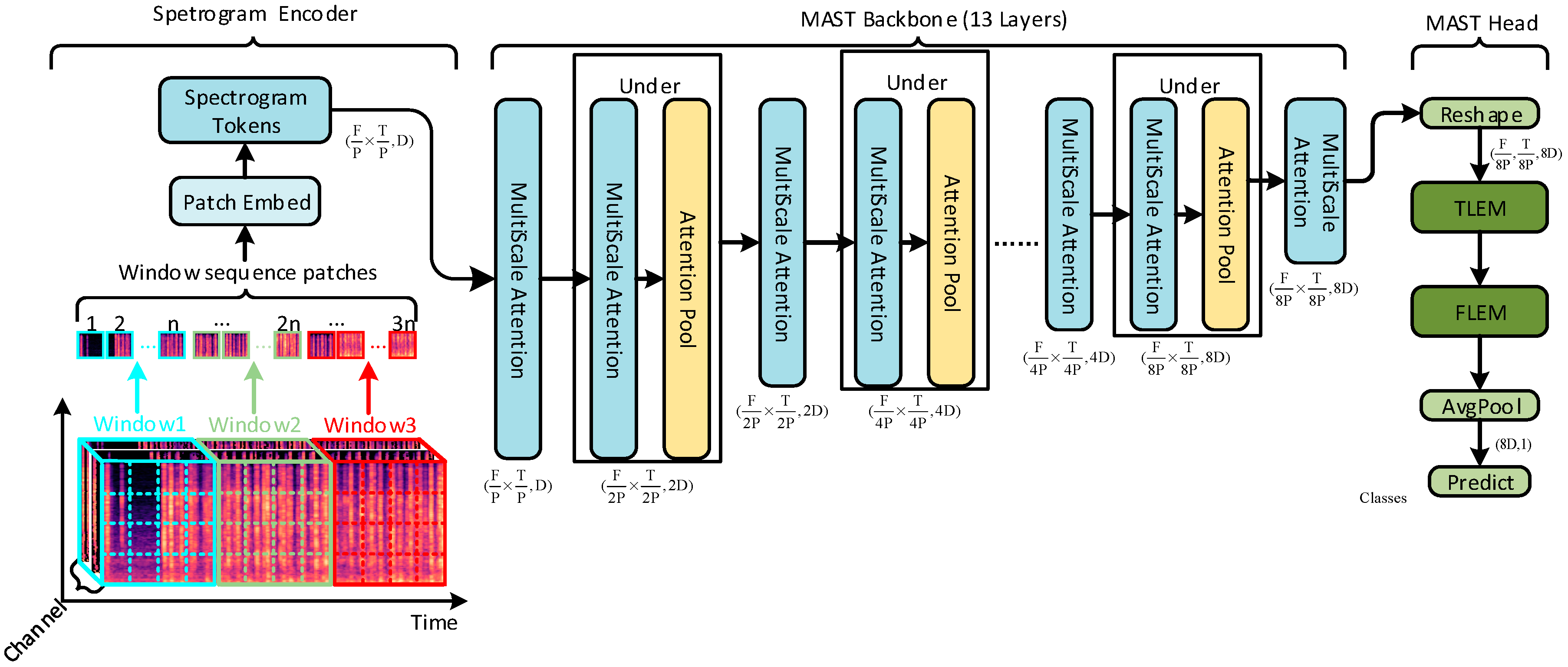
3.1. Model Overall Architecture

Model Input: Firstly, the original audio file was resampled, framed, windowed, put through STFT, Mel frequency scaling, logarithmic calculation and other steps to obtain the Log-Mel spectrogram, on which delta and delta-delta features were calculated. The above features were concatenated in the channel dimension to form input data with three-dimensional features, which were then sent to the backbone network.
Spectrogram Encoder: An audio spectrogram kernel of size (P × P) was cut into different spectrogram tokens by a Patch-Embed CNN and used as input to the MAST backbone. The audio spectrogram representation was different from the conventional RGB image. The width and height of the audio spectrogram represented the time and frequency dimensions, respectively, and the channel dimension was a multi-feature representation (static, delta, delta-delta). Since the time dimension of the multi-channel spectrogram was longer than the frequency dimension, to capture the relationship of spectrogram patches between frequency bands at the same time, the Mel spectrogram was partitioned into windows w1, w2, w3, etc. The local regions within each window were then patched and embedded to obtain the final spectrogram tokens feature representation.
MAST Backbone: The backbone network was used for feature extraction and consisted mainly of multi-scale self-attention blocks. The most critical part of the multiscale self-attention module was the pooling attention process, which reduced the computational complexity of self-attention by pooling attention, and upscaled the feature representation of each token, as described in Section 2.3. As the network deepened, the pooling mechanism removed redundant spectrogram markers through maximum pooling, while progressively reducing the complexity of the computation in a self-care calculation. In the code implementation, a multiscale Transformer block [51] with a multi-scale hierarchy was used, which was a more efficient mechanism for multiscale global attention. It was helpful to deploy pretrained multiscale Transformer vision models in the experimental phase.
MAST Head: After obtaining the global representation through the Backbone, MAST prediction head projected the class of the speech spectrogram. Time-level Local Enrichment Module and Frequency-level Local Enrichment Module were designed in the prediction head. Using the overall framework of global + local, the importance of local time-frequency features was emphasized in the global feature representation, as described in Section 3.4.

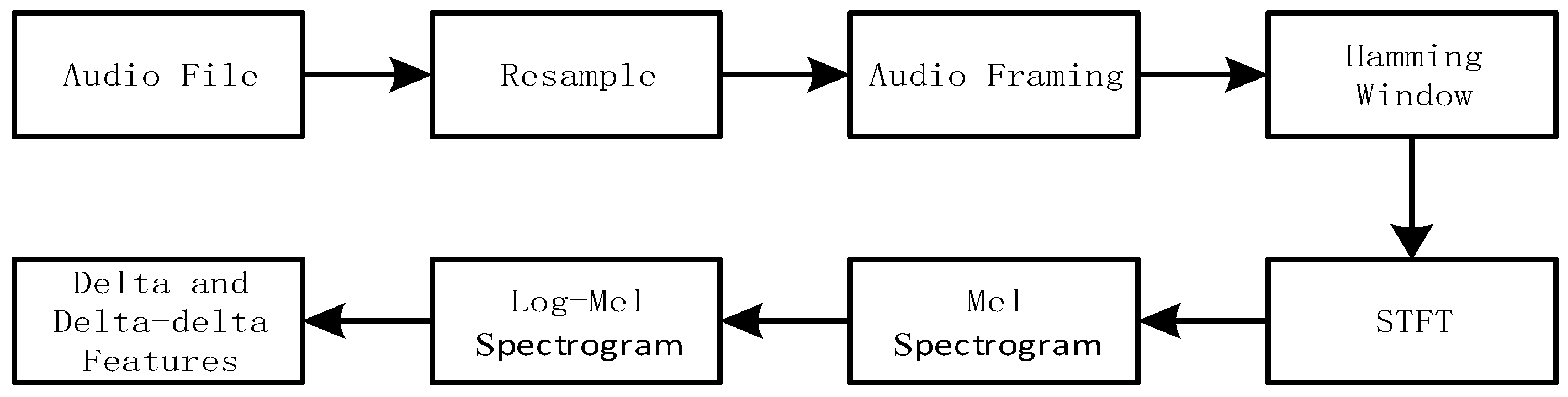
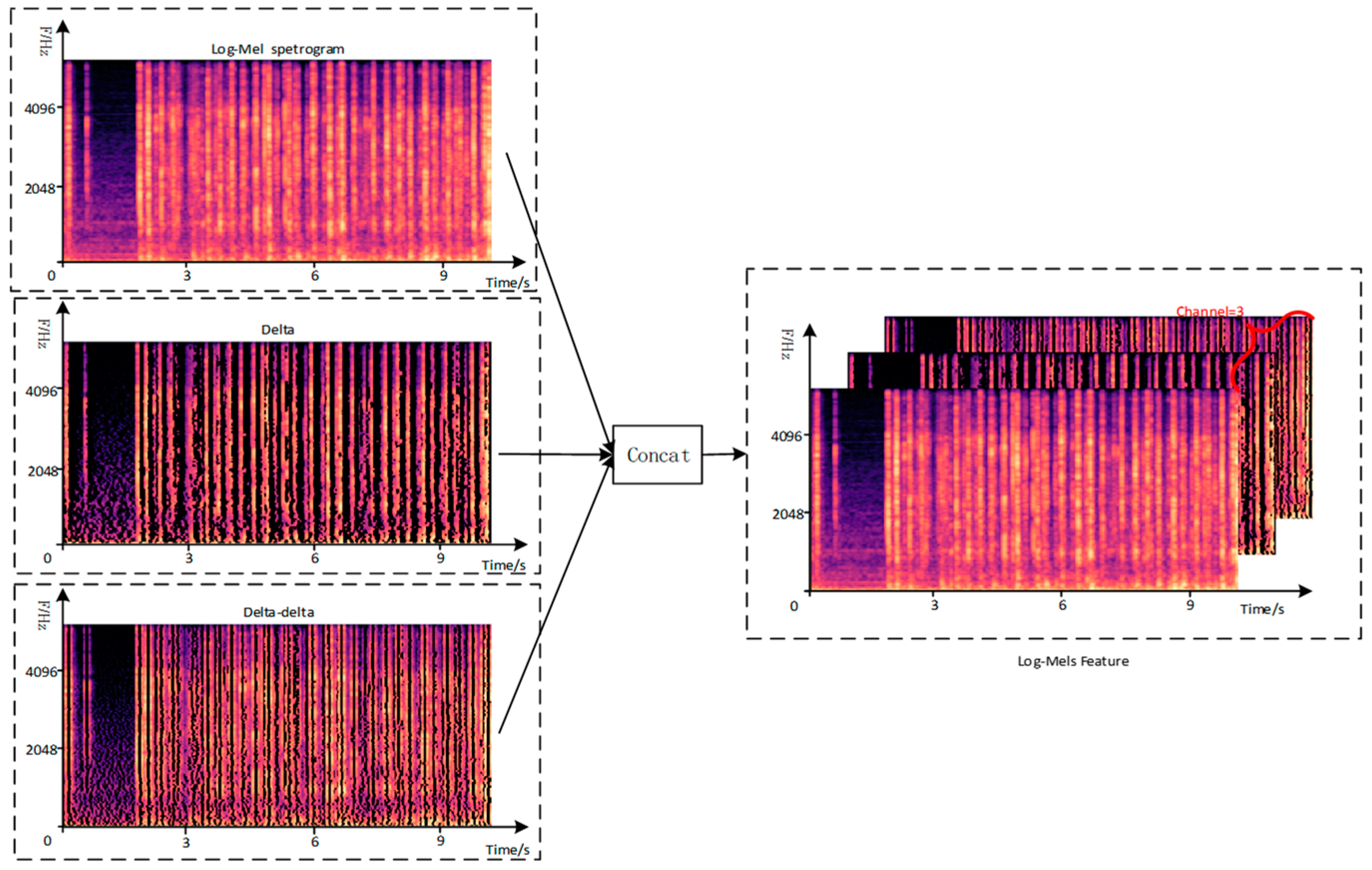
3.2. Multi-Channel Spectrogram Feature Construction

Time and frequency domain analysis are both of the most important methods for speech signals. The Log-Mel spectrogram combines the advantages of these two analysis methods and uses a deep model to learn its advanced features. Log-Mel spectrogram contains a variety of acoustic information such as formant, fundamental frequency, energy, amplitude, etc., which is more intuitive to understand and easier to extract features with the neural network than with the original speech signal. Log-Mel spectrogram contains a variety of acoustic information such as formant, fundamental frequency, energy, amplitude, etc., which is more intuitive to understand and easier to extract features by the neural network than the original signal. Therefore, Log-Mel spectrograms are used as model input data in this paper. However, existing audio transformer [25,40,41] methods use individualized features as input and audio classification performs differently. To overcome this problem, we used Log-Mels with deltas and delta-delta as input to the MAST model.
The Log-Mel Spectrogram was constructed through the process in Figure 2. First, the deltas feature m i d of the Log-Mel spectra was calculated and the Log-Mel feature m i was operated on using Formula (1). Similarly, the delta-delta feature m i d d was calculated by taking the time derivative of delta, as shown in Formula (2). Concatenate the obtained Log-Mel, delta and delta-delta features in the channel dimension, and finally obtained a three-dimensional feature representation X R t × f × c where t represents the length of the time frame, f represents the number of Mel-filter banks and c represents the feature number of channels. The extracted multichannel Log-Mels features are shown in Figure 3.
m i d = n = 1 N n ( m i + n m i n ) 2 n = 1 N n 2
m i d d = n = 1 N n ( m i + n d m i n d ) 2 n = 1 N n 2

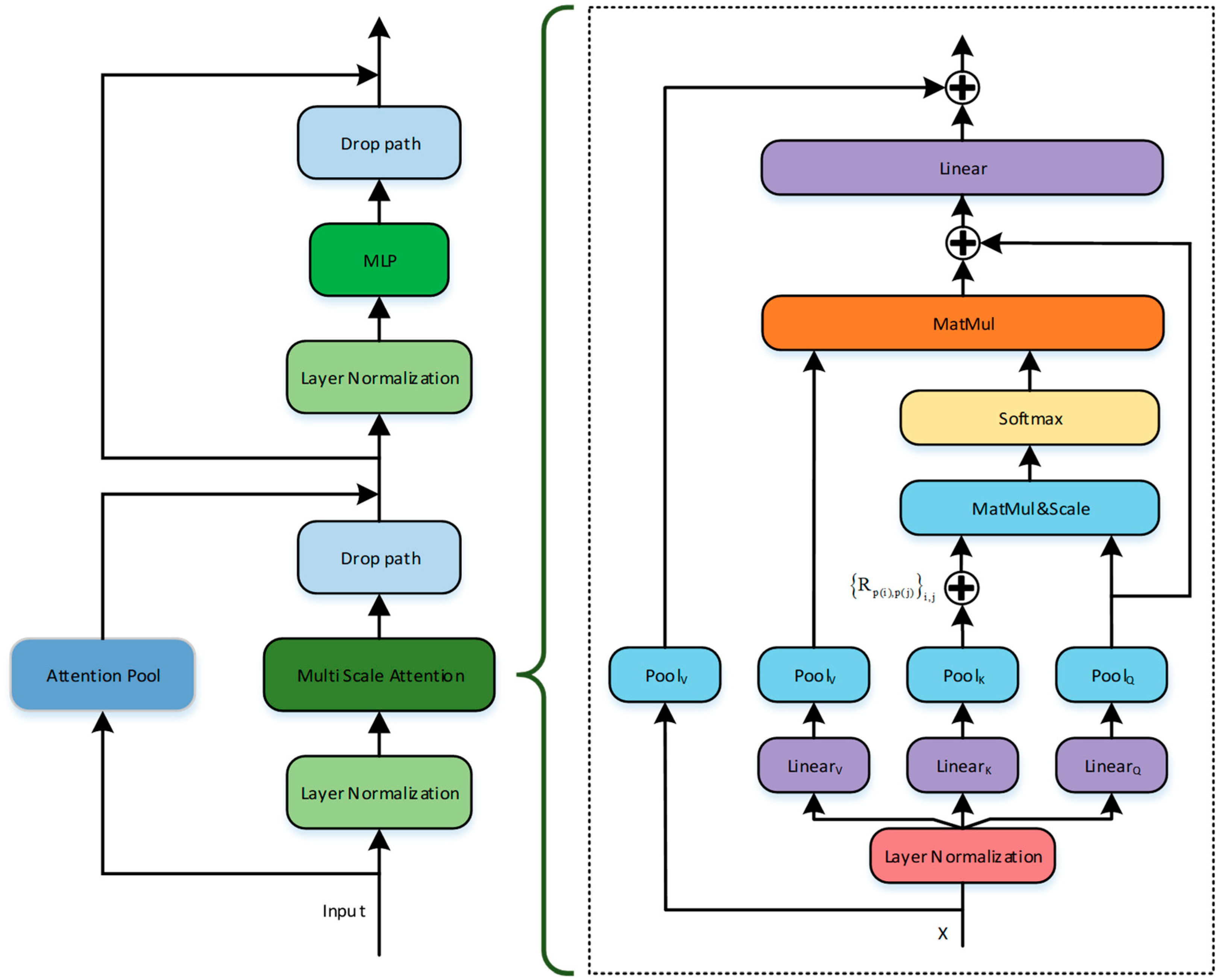
3.3. Multi-Scale Audio Spectrogram Transformer

3.3.1. Pooling Attention

Similar to traditional convolutional networks, the network construction process continuously reduces the time-frequency resolution and increases the channel dimensions, in which Multi-Head Pooled Self-Attention (MHPSA) is the basis for flexible scaling, and each Transformer block contains Multi-Head Pooled Self-Attention (MHPSA). The left part of Figure 4 is a single Multi-scale Audio Spectrogram Transformer block, where Multi-Head Pooled Self-Attention (MHPSA) is shown in the right half of Figure 4. Unlike AST [25], in which the channel dimension and the time-frequency resolution are kept constant, MHPSA pools the feature tensor to reduce the sequence length of the data. For a specific MHPSA, the input tensor X L × D goes through a linear layer mapping tensor of Q ^ , K ^ , V ^ , the weight dimension of the linear layer is D × D and the output mapping tensor is still L × D .
Q ^   = X W Q K ^   = X W K V ^ = X W V
The pooling convolution is next computed in each dimension using 𝒫 ( · , Θ ) for Q ^ , K ^ , V ^ . Θ denotes the use of a pooling kernel with parameter (k,s,p), k denotes the size of the pooling kernel, s is the pooling kernel step size, p is the pooling padding scale and the pooled sequence length L ˜ is as in Formula (4). For the individual Q ^ , K ^ , V ^ intermediate tensor, the pooling operation produces the pooled scaled Q = 𝒫 ( Q ^ , Θ Q ) , K = 𝒫 ( K ^ , Θ K ) and 𝒫 V = ( V ^ , Θ V ) . The pool attention is calculated as in Formula (5), E ( r e l ) is the relative position encoding and d is used for row-by-row normalization of the inner product matrix.
L ˜ = L + 2 p k s
Attention ( Q , K , V ) = Softmax ( 𝒫 ( Q ^ , Θ Q ) 𝒫 ( K ^   , Θ K ) T + E ( r e l ) / d ) 𝒫 ( V ^   , Θ V )
Different from the traditional single invariant scale attention calculation (NA) in AST, in the pooling attention calculation (PA) the time-frequency resolution is continuously reduced in the Transformer block. Thus, the corresponding reduction in computational complexity and s Q , s K , s V are the scaling factors for the time-frequency resolution. The computational complexity of the two mechanisms for an audio patch tagging of f × t with data dimension D is:
N A : O ( f t D 2 + ( f t ) 2 D )
P A : O ( f t D 2 + ( f t ) 2 s Q s K D )
where pooling attention reduces the second complexity term by a factor of s Q s K . As the network deepens, the pooling attention module extracts key audio patch tokens by filtering, keeping the relationships calculated in consecutive frequency bands and time frames across the global range.

3.3.2. Multi-Scale Audio Spectrogram Transformer Network

Multi-scale Audio Spectrogram Transformer Network was constructed by the above MHPSA and Multilayer Perceptron (MLP), and the specific detailed settings are shown in Table 1. The network mainly consists of four attentional computation stages of scale features, where each scale stage contains N superposition processes of MHPSA and MLP. For simplicity of representation in Figure 1, the complex process of each scale stage will be Multi-scale Attention.
By encoding the multi-channel Log-Mels feature, ( T P × F P , D ) is obtained in the Patch-Embed process, where P is 4 and D is 96. The single-scale operation contains several Transformer blocks at the same time-frequency resolution and channel dimension D. In the scale stage, each block includes MHPSA, MLP and Layer Normalization (LN) operations, and the computation is performed as follows:
X 1 = M H P S A ( L N ( X ) ) + 𝒫 ( X )
B l o c k ( X ) = M L P ( L N ( X 1 ) ) + X 1
As shown in the right part of Figure 4, the dimension of the feature tensor is the same at the same stage, and the Attention Pool operation of the P representation is a direct residual connection. When the stage changes, P represents the maximum pooling operation to ensure the executability of the residual connection. Additionally, at the end of each stage, the channel dimension is expanded by the MLP, especially when scale 2 crosses scale 3, the time-frequency resolution is reduced by a factor of 2 and its channel dimension is increased to a factor of 2.

3.4. Time-Frequency Domain Local Enrichment Module

Since the spectrograms have a different meaning from the dimensional information in conventional visual images, where the pixel feature scale is X, H is the height of the image, W is the width of the image and C is the number of RGB three channels of the image, the Log-Mels axis we constructed represents different dimensions, i.e., frequency, time and number of channels. Simply applying Transformers directly to spectrograms and global attention calculations for spectrogram patch is imperfect; a better approach is to separate the time and frequency axes for local enrichment on the basis of global modeling.

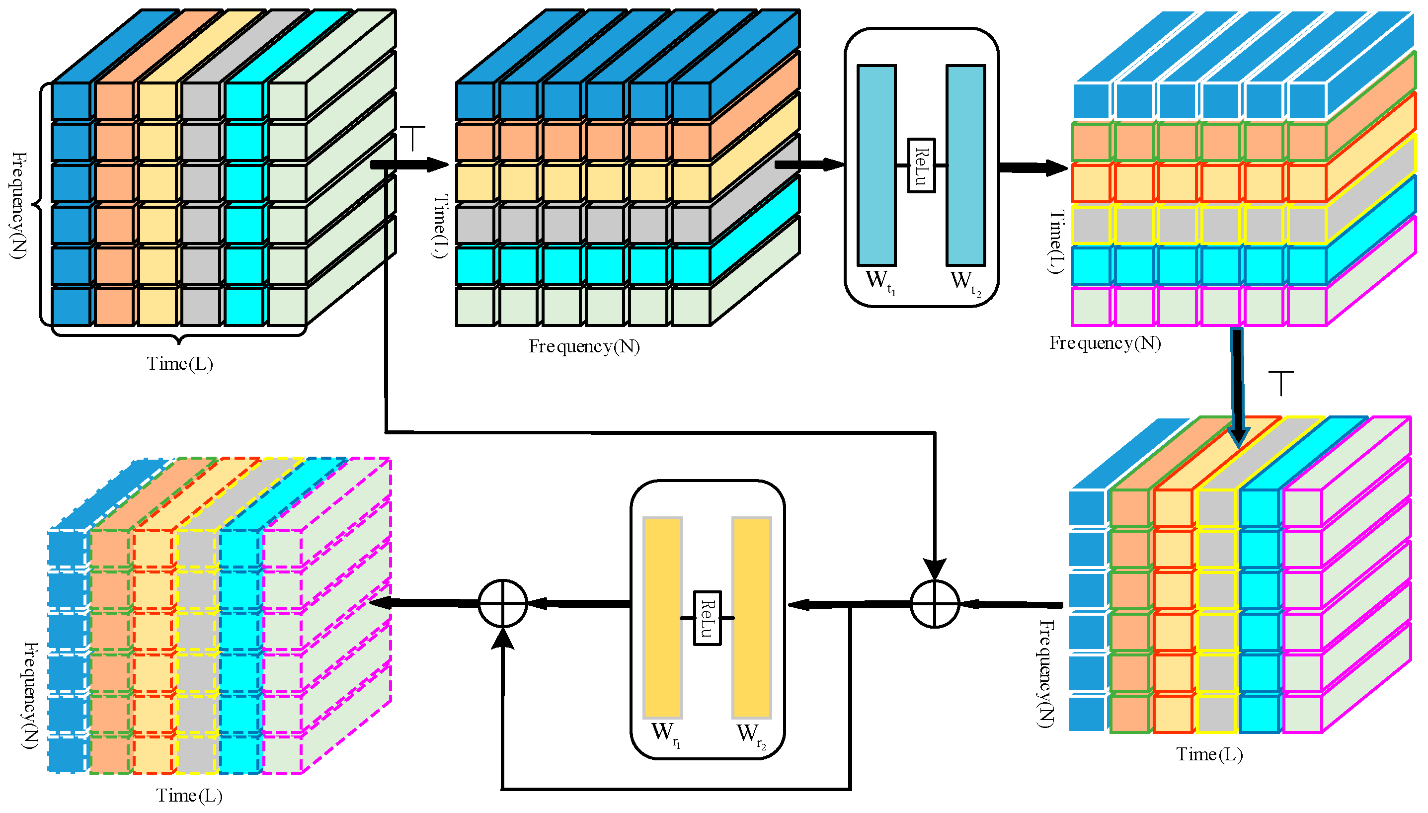
3.4.1. Time-Level Local Enrichment

Traditional Audio Transformer methods use cls tokens to predict audio classification results, which do not make use of the time and frequency band information contained in each token in the final layer. The above-mentioned Multi-scale Transformer can aggregate the time-frequency context of the global range into the tokens of Log-Mels. However, it cannot encode individual time-frame down tokens in a specific way, so it gets into trouble if a key time-frame speech feature has a distinctive character. For example, the sound that occurs at a certain period may determine the category of this sound sample, and we pay attention to this. A Time-level Local Enrichment Module (TLEM) was designed by adjusting the MLPmixer to assimilate the local domain within a single time frame by an input-independent, persistent relational memory for the completed tokens-mixing within that time frame. the TLEM module is shown in Figure 5.
For the output tensor X L × D of MAST, it is adjusted in the time-frequency domain to Y T × F × D by separately characterizing the global tensor V = [ v 1 ; ; v F ] T × F × D in the time dimension, where v i F × D denotes a sequence of tokens at different frequencies at the same time, which is then processed by the TLE module. First, the temporal tokens of h i are blended through a two-layer MLP W t ( · ) that is shared across channels (feature dimensions). Subsequently, the intermediate feature h is tokens refined using another two-layer MLP W r ( · ) , which is shared across tokens, and two mixing operations in TLE as shown in Formulas (10) and (11).
V * = σ ( V T W t 1 ) W t 2 + V T
V T = σ ( V * T W r 1 ) W r 2 + V * T
V T T × F × D is a locally enriched feature for the time dimension, W t 1 , W t 2 F × F and W r 1 , W r 2 D × D are trainable parameters for token and channel mixing and σ denotes the ReLU activation function.

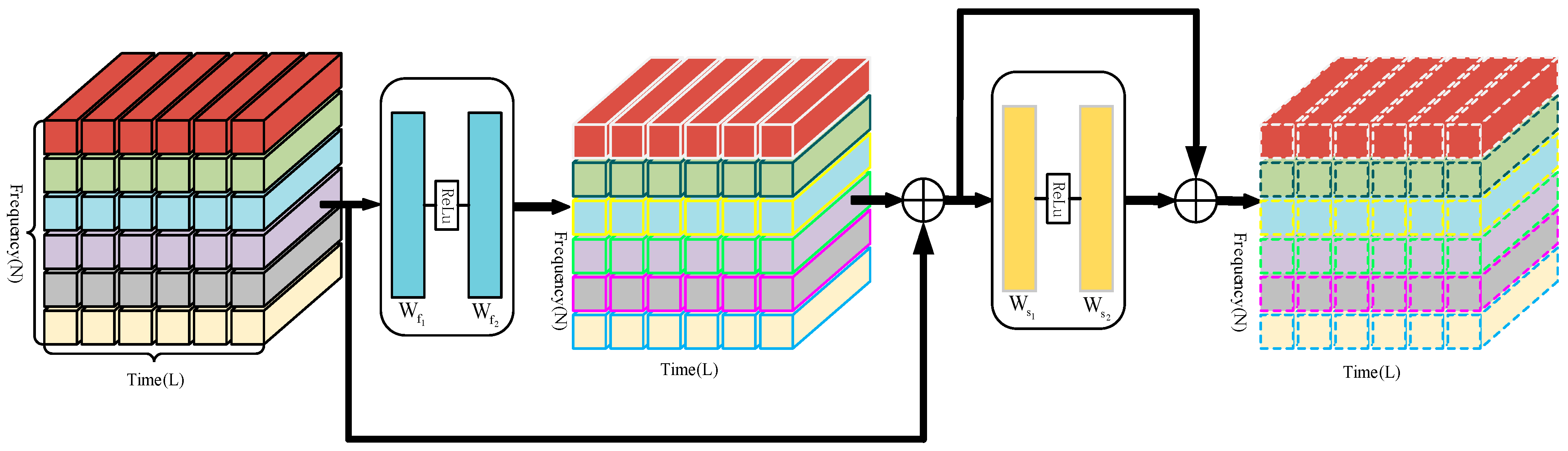
3.4.2. Frequency-Level Local Enrichment

The enrichment of tokens for only a single time frame is incomplete, as it does not take into account the frequency enrichment of the backbone output. In a similar way to the TLE module, we developed a module for the frequency-level local enrichment (FLE) in the horizontal direction, focused on the temporal variation of features in high-dimensional spectrograms with fusion of multiple temporal tokens at the same frequency. The same audio fluctuates less in the frequency domain and the FLE module is able to capture the temporal features of the same audio frequency. The FLE module is shown in Figure 6.
The input tensor X L × D of the FLE module was derived from the output of the TLE module. Due to the computational nature of the neural network, there was no need to transform the feature dimension of the input tensor. By characterizing the global tensor H = [ h 1 ; ; h T ] T × F × D separately in the frequency dimension, h i F × D represents a sequence of tokens at different times in the same frequency band, which was then processed by the FLE module. Next, tokens refinement of the intermediate feature H * was performed after another two-layer MLP W s ( · ) , which was shared across tokens. Two mixing operations in frequency-level local enrichment are shown in Formula (12) and (13).
H * = σ ( H W f 1 ) W f 2 + H
H T = σ ( H * W s 1 ) W s 2 + H *
H T T × F × D is a local enrichment of features for the frequency dimension and W f 1 , W f 2 F × F and W s 1 , W s 2 D × D are trainable parameters for tokens and channel mixing.

4. Experimental

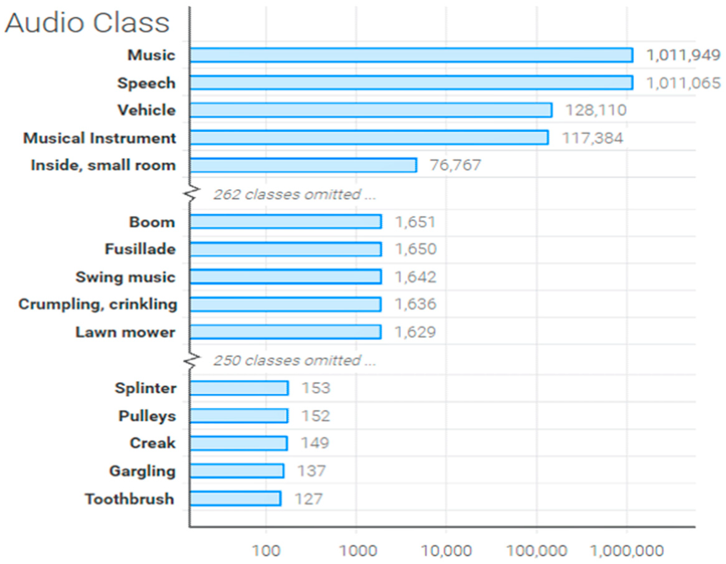
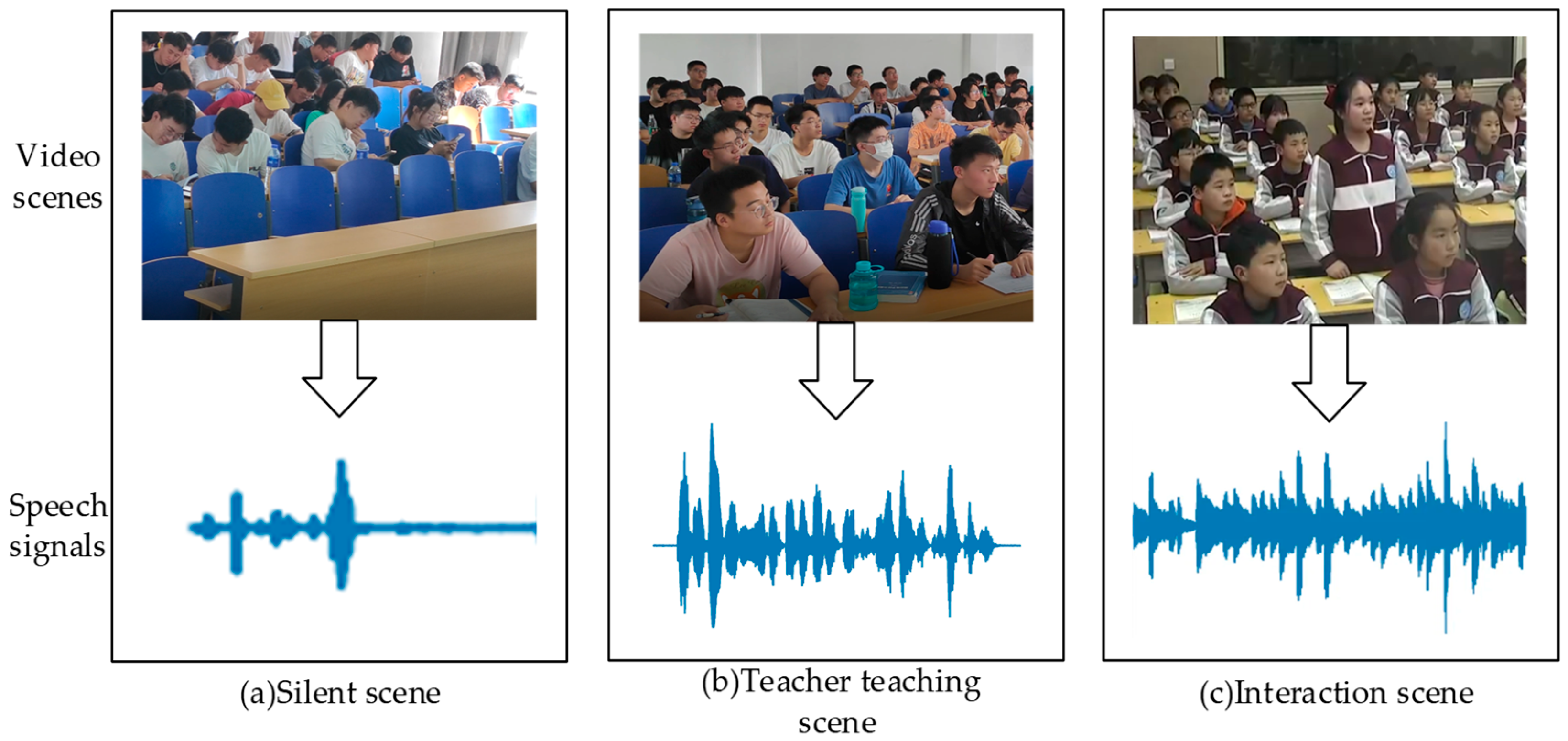
4.1. Datasets and Production

AudioSet: Audioset contains over 2 million audio samples labeled into 527 sound event categories, derived from a collection of human-labeled 10 s sound clips extracted from YouTube videos. Audio genres cover a wide range of human and animal sounds, instruments and genres, as well as common everyday ambient sounds. In this paper, we adopt the same training pipeline as in [25]. The training set adopted the full-train set with 2M samples, and the validation set contained 22K samples for evaluation. All samples were audio data sampling at 32 kHz sampling rate. Some audio sample distributions are shown in Figure 7. Data augmentation plays a very important role in improving performance, especially in the case of deep models where data are scarce, and can improve the generalization of the model. The data augmentations used include balance sampler [52], α = 0.5 mix-up, spectrogram masking [53], with time-mask = 128 frames and frequency-mask = 16 bins, etc.
ESC-50: ESC-50 [48] is one of the most popular environmental sound classification benchmark datasets, consisting of a collection of 2000 audio samples, each 5 s long, sampled at 44.1 kHz, recorded in a single channel. It contains five categories: animal sounds, natural landscapes and water sounds, human communication sounds, indoor/outdoor sounds and indoor/outdoor noise, each of which includes 10 subcategories. In total, there are 50 different environmental sounds, which basically cover the common environmental sounds in daily life. For the evaluation, we used the 5-fold cross-validation.
CSID: Existing audio classification datasets are used to detect specific categories in generic scenarios, but there is no common dataset for teacher–student interaction states in the classroom. Therefore, this paper captures audio in real classroom scenarios and manually constructs a Classroom Speech Interaction Dataset (CSID), which contains three major categories: teacher teaching (single voice, lecture), teacher–student interaction (teacher–student communication, group discussion) and silence (silent scene). The various classroom audio capture scenarios are shown in Figure 8. Capturing video data alongside classroom speech data helped to segment the audio for the actual scene.
Existing audio classification datasets are used to detect specific categories in generic scenarios, but there is no common dataset for teacher–student interaction states in the classroom. The datasets were captured at fixed time frame intervals, with each audio segment being approximately 10 s. These audio samples were filtered out of unimportant before-and-after changes and the ffmpeg tool was used to crop each data sample to produce wav audio files. Each piece of audio was placed in a folder with the corresponding category name. A total of 3682 tags were tagged, and the training and test sets were divided 8:2. The number of each tag is shown in Table 2.

4.2. Experimental Equipment and Evaluation Metrics

The experimental platform for this paper was Ubuntu 20.04 operating system, the CPU was Intel(R) CORETM i9-10900k [email protected], the deep learning computing graphics card was GeForce RTX A5000 with 24 GB video memory size and the audio recognition model was built using the deep learning framework Pytorch version 1.8.0 based on Python environment 3.7.0.
At the same time, in order to evaluate the effectiveness of the algorithm at the objective index level, the evaluation index used mAP (mean average precision) and classification accuracy (Accuracy) to evaluate the performance of the algorithm in this paper. The calculation formula of specific indicators is as follows:
A c c u r a c y = T P + T N T P + T N + F P + F N
mAP = j = 0 n A P ( j ) n
where TP, TN, FP and FN represent the number of positive samples correctly predicted, the number of negative samples correctly predicted, the number of incorrectly predicted samples and the number of missed detections, respectively, and AP(j) is the average precision of the jth category of samples.

4.3. Experimental Results and Analysis

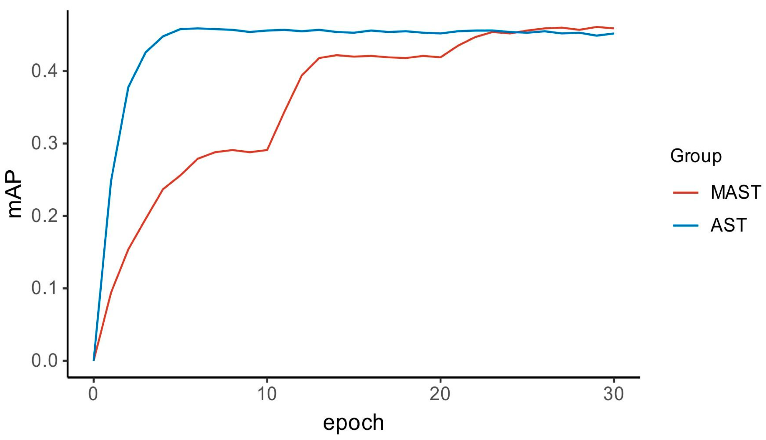
4.3.1. Experimental Results of Event Classification on AudioSet

This paper begins with experimental validation on large-scale data to illustrate the advantages of the MAST model’s ability to model with fully fitted parameters. As AudioSet has 2 million data samples, which matches the data sample size required for the experiments, the specific data pipeline was used in the same way as in [25]. We trained the model using the Adam optimizer with an initial learning rate of 1 × 10⁻⁴. A total of 30 epochs were experienced by setting the learning decay coefficients to [0.1, 0.05, 0.02], with the first 3 epochs used for warm-up training. Finally, mAP was used as our main evaluation metric. For the extraction of audio features, the frame length of each frame was set to 1024, the frameshift to 320, the number of filter banks to 64, the sampling rate 32 kHz, the audio length was unified to 10 s and all feature vectors were normalized to the 0 to 1 interval.
The results of the mAP curves of the proposed network model and the AST model are compared in Figure 9. It can be seen that the average accuracy of the algorithm has improved significantly compared with the AST algorithm. When the algorithm in this paper was iterated to the 23rd epoch, the mAP increased to about 0.457, and finally in a steady rise to about 0.461; when the AST algorithm was iterated to the 5th epoch, the mAP only increased to about 0.458, the model overfitting phenomenon occurred in the subsequent training process and the model mAP accuracy kept oscillating and decreased to some extent.
To verify that the proposed method is advanced in the field of audio classification, the algorithms in this paper are compared with the mainstream audio classification algorithms, and to ensure fairness, all models are trained in the full_train method on Audi-oSets data and tested for comparison.
Table 3 shows the results of comparing our model with other representative state-of-the-art methods. The previous best accuracy on the AudioSet dataset is 0.459, while our proposed MAST can achieve 0.461, which is an improvement of 0.002 compared with the previous best result, but the number of model parameters in MAST is significantly lower compared with AST. Compared with other CNN-attention hybrid models, the algorithm in this paper may be higher in terms of the number of model parameters, because the method is based on the transformer architecture, which also enables a significant improvement in detection accuracy and achieves a balance between detection accuracy and model complexity.
To show the effectiveness of the multi-channel features and the Time-Frequency Domain Local Enrichment Module proposed in this paper, ablation experiments were conducted on a large-scale AudioSet dataset. The results are shown in Table 4.
As shown in Table 4, the Multi-scale Transformer trained with only a single feature as input, due to its relatively small input feature map factor, and obtained an effect of 0.451. Compared with several types of models based on CNN-attention, it has achieved a better result than the current state of CNN-based methods. The accuracy was raised to 0.454 by replacing the single feature map with multi-channel features, suggesting that multi-channel features provide richer underlying information for model classification to aid identification. The subsequent addition of TLEM and FLEM to the base network improved the classification accuracy by 0.003 and 0.004, respectively, which exceeded most methods at this stage, indicating that the output layer features of the base network contain information about their corresponding time-frequency bands. The method of training enrichment attention weights on their time-domain and frequency-domain information, respectively, followed by pooling and fusion, is useful for improving audio classification accuracy. The analysis of the ablation experimental results shows that both the multi-channel features, the Time-Frequency Domain Local Enrichment Module and the Multi-scale Transformer methods help to improve the classification ability of the model.

4.3.2. Experimental Results of Event Classification on ESC-50

In this paper, experimental validation is carried out on small sample data to illustrate the continued strength of the MAST model in the face of data limitations. The small scale data are the ESC-50 dataset. The data were divided into 5 folds, of which 4 folds were selected as the training set and 1 fold was selected as the test set for a total of 5 training sessions. The experiment was repeated 3 times using random seeds to obtain the average accuracy. The dataset was evaluated using the Accuracy. During the experimental data processing, the audio samples from ESC-50 were resampled and the sampling rate was set to 32 kHz, with the same specific experimental parameters as the AudioSet dataset.
To verify that the proposed method has good classification accuracy even when the models are data-limited, various audio classification models were trained without pre-training the models on the AudioSet dataset. To ensure fairness, all algorithms in the experiments used the same training parameters and training samples, and the experimental results are presented in Table 5.
As can be seen from Table 5, the recognition accuracy of MAST in this paper is higher than other algorithms when MAST is trained directly on the ESC-50 dataset, while the number of model parameters of the method is reduced relative to other algorithms. Since PANN and EfficientNet are convolutional neural network-based methods, the model is limited to achieving higher accuracy because the convolutional computation is often limited to the convolutional window size. AST, SepTr and our MAST are the recently emerged Vision Transformer-based models that tend to achieve the accuracy of MAST and SepTr 92.0 and 91.1, respectively. The reason for the lower accuracy of AST is that it is a more complex model and the fit is often not as good as it could be given the data constraints.
In this paper, the proposed algorithm is pre-trained on AudioSet first, and the prediction accuracy is further improved in the small-scale ESC dataset by transfer learning. The experimental comparison results based on transfer learning are shown in the lower part of Table 5, where the pre-trained MAST model obtained an accuracy rate of 96.1.
Figure 10 shows the confusion matrix generated by the pre-trained transfer method of this paper on the ESC-50 dataset. As can be observed, the best method in this paper accomplishes a high-accuracy classification of environmental sounds in ESC-50. The sound categories in this dataset contain 50 classes, using a numerical label form to represent specific label categories inside the dataset.
As can be seen from Figure 10, the classification accuracy of the MAST (pretrain) method for all environment audio was above 87.5% and reached 100% classification accuracy for multiple category labels such as No. 1, 17, 20, 39, and 40. However, due to the similarity of sound between some of the categories, it is easy to confuse the process of sound recognition. A typical misclassified sample such as the 47th sample label category has five audio samples incorrectly identified as the label category of No. 40, which correspond to the real labels of aircraft sound and helicopter sound, respectively, and their similarity and easy-to-confuse characteristics cause the model to misidentify.

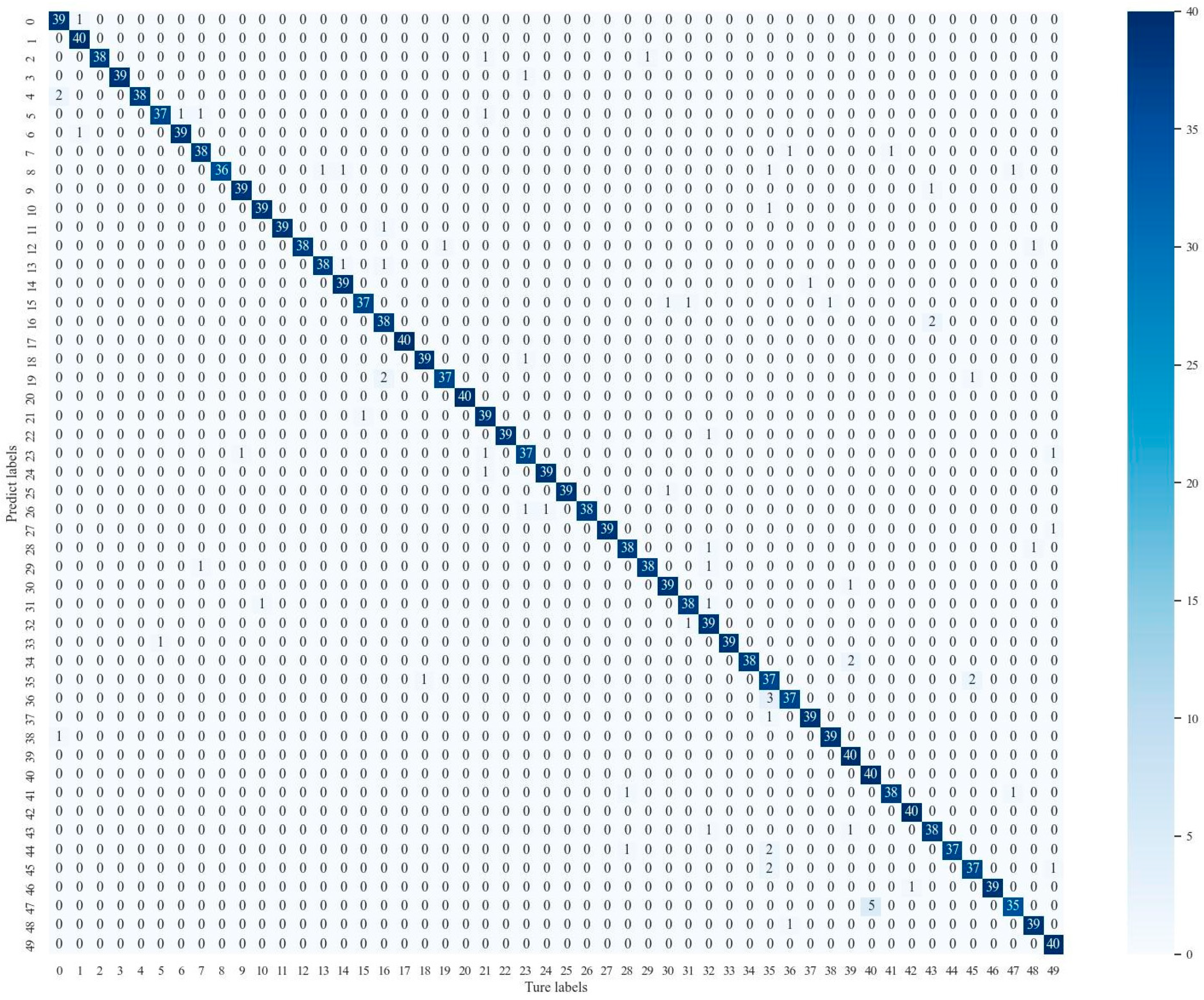
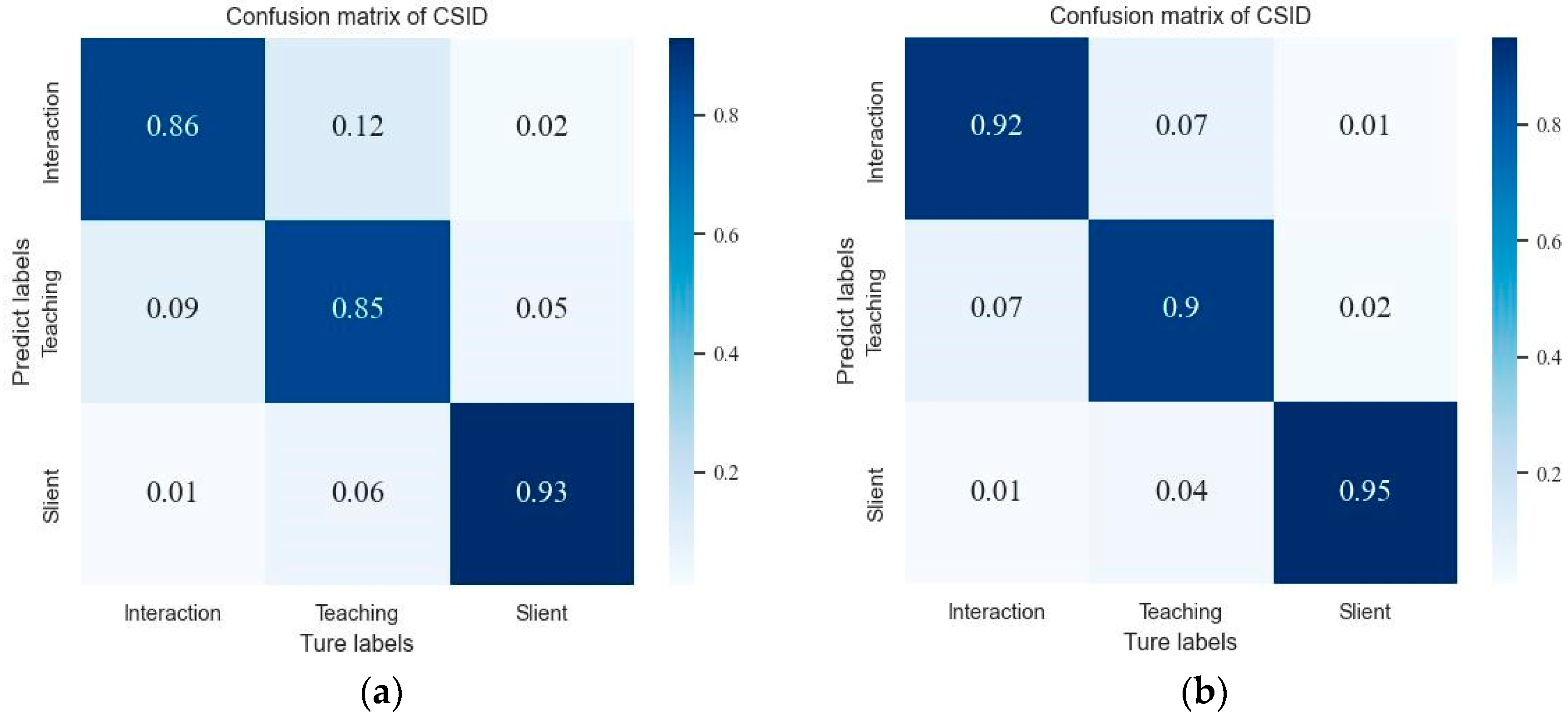
4.3.3. Experimental Results of Event Classification on CSID

Finally, we transferred the proposed audio classification model in this paper to the classroom interaction recognition domain for experimental validation in a self-built CSID dataset. To avoid chance in the experiments, each set of experiments was conducted three times and the experiments were repeated three times using random seeds to obtain the average accuracy. For the experimental data processing, the experimental parameters such as sampling rate were consistent with the ESC-50 and AudioSet datasets, except for the frameshift parameter, which was set to 640.
Since some codes of the above methods are not publicly available, we selected representative methods from the public methods for experimental comparison. Table 6 shows the Accuracy and Average accuracy of the different models for the three categories in CSID, as well as the model-related parameters. It can be seen that the MAST model, when applied to speech interaction recognition in the classroom, has higher accuracy than other algorithms. It is worth noting that even without pre-training on the AudioSet dataset, MAST still outperforms the PANN and AST methods by 2.4% and 2.8%, respectively.
When comparing different categories of recognition, our model still achieved the highest accuracy in each category. However, all types of methods tend to have lower accuracy in the recognition of the Teaching and Interaction categories, which is greatly alleviated by the pre-trained MAST method. The confusion matrix generated by MAST on the CSID dataset is shown in Figure 11 for this case.
As can be seen from Figure 11, the classification accuracy of the Silent scenes tends to be higher, especially as the pre-trained MAST obtained a recognition rate of 95%. However, there are still confusion-prone Teaching scenes and Interaction scenes in Figure 11b, where 7% of the samples of the Teaching scene are identified as Interaction scenes, and 7% of the samples of Interaction scenes are identified as Teaching scenes. The analysis of the samples shows that some transient Interaction scenes are easily misidentified as Teaching scenes, while audio interference from outside the classroom can easily lead to misidentification in Teaching scenes. Therefore, by eliminating audio interference from outside the classroom, exploring classroom audio noise reduction methods, and combining the MAST model with the advantages of high accuracy and fewer parameters in classroom tasks, the intelligent classroom recognition method can be more practical.

5. Conclusions

In this paper, we propose a model MAST for audio scene recognition and transform the classroom interaction detection problem into a classification problem of classroom speech interactivity. We design multi-channel spectrogram features to effectively characterize the multi-dimensional features of audio and to explore the detailed features of audio; by introducing a multi-scale Transformer network, we strengthen the model’s ability to compute the global attention of the audio spectrogram at different scales; finally, the Time-Frequency Domain Local Enrichment Module captures the temporal dynamic features and concurrent features of the sound, enhancing the local modeling at the time and frequency domain levels.
The MAST algorithm proposed in this paper can accurately identify classroom interaction scenes with higher accuracy and robustness for generic audio classification datasets. Experiments under the evaluation protocol of common scene classification datasets AudioSet and ESC-50, show that MAST achieves the accuracy of advanced methods compared with CNN and traditional Transformer. Ablation experimental analysis shows that multi-channel features and Time-Frequency Domain Local Enrichment Module are important modules. At the same time, the use of the Multi-scale Transformer reduces the number of model parameters and achieves the goal of further lightweight and efficiency of the model while ensuring the accuracy of classroom interaction recognition in the self-built dataset, which is more in line with the requirements of practical production applications.
While the results are encouraging, the application of this work is also limited. Firstly, classroom audio is susceptible to interference from other classroom or outdoor factors, making it difficult to obtain data for the ideal collection of classroom interactions. Secondly, our method only considers teacher–student verbal interactions during classroom interactions. However, in practice, classroom interactions may include a small number of teacher–student behavioral interactions. The traditional lecture-based classroom differs from the interactive practice classroom in that the interaction between teachers and students in the classroom is verbal knowledge exchange, and the traditional lecture-based classroom can be judged by verbal interaction.
This research has the following potential applications and further developments in the classroom scenario. By deploying audio capture devices in the classroom connected to a backend server and porting interaction recognition algorithms, classroom interactions can be recorded and presented automatically. The education system completes an automatic analysis and evaluation based on the frequency and proportion of interactions within the classroom at each period. If the proportion and frequency of weak interactions exceed certain thresholds, the teacher is advised to improve the teaching strategy of the classroom. In future work, we will consider combining classroom behavior recognition algorithms with learning emotion recognition algorithms. Adding teacher–student interaction behavior and emotional states in learning to classroom assessments enables smart classroom algorithms with more integrated assessment results and richer use of classroom scenarios.

Author Contributions

Supervision, J.F.; conceptualization, F.L. and J.F.; formal analysis, F.L. and J.F.; methodology, F.L.; software, F.L.; writing—original draft, F.L. All authors have read and agreed to the published version of the manuscript.

Funding

This research was funded by the Inner Mongolia Natural Science Foundation Project under grant number 2019MS06023, The Basic Scientific Research Business Expense Project of Inner Mongolia Universities under grant number JY20220012 and the Inner Mongolia Science and Technology Plan Project under grant number 2022YFSJ0034.

Data Availability Statement

The data presented in this study are available on request from the corresponding author. The data are not publicly available due to privacy restrictions.

Conflicts of Interest

The authors declare no conflict of interest.

References

  1. Solis, O.J.; Turner, W.D. Strategies for Building Positive Student-Instructor Interactions in Large Classes. J. Eff. Teach. 2016, 16, 36–51. [Google Scholar]
  2. Solis, O.J.; Turner, W.D. Building positive student-instructor interactions: Engaging students through caring leadership in the classroom. J. Empower. Teach. Excell. 2017, 1, 4. [Google Scholar]
  3. An, J.; Macaro, E.; Childs, A. Classroom interaction in EMI high schools: Do teachers who are native speakers of English make a difference? System 2021, 98, 102482. [Google Scholar] [CrossRef]
  4. Flanders, N.A. Intent, action and feedback: A preparation for teaching. J. Teach. Educ. 1963, 14, 251–260. [Google Scholar] [CrossRef]
  5. Khalil, R.A.; Jones, E.; Babar, M.I.; Jan, T.; Zafar, M.H.; Alhussain, T. Speech emotion recognition using deep learning techniques: A review. IEEE Access 2019, 7, 117327–117345. [Google Scholar] [CrossRef]
  6. Yoon, S.; Byun, S.; Jung, K. Multimodal speech emotion recognition using audio and text. In Proceedings of the 2018 IEEE Spoken Language Technology Workshop (SLT), Athens, Greece, 18–21 December 2018; pp. 112–118. [Google Scholar]
  7. Mushtaq, Z.; Su, S.-F. Environmental sound classification using a regularized deep convolutional neural network with data augmentation. Appl. Acoust. 2020, 167, 107389. [Google Scholar] [CrossRef]
  8. Tripathi, A.M.; Mishra, A. Environment sound classification using an attention-based residual neural network. Neurocomputing 2021, 460, 409–423. [Google Scholar] [CrossRef]
  9. Eyben, F.; Weninger, F.; Gross, F.; Schuller, B. Recent developments in opensmile, the munich open-source multimedia feature extractor. In Proceedings of the 21st ACM International Conference on Multimedia, Barcelona, Spain, 21–25 October 2013; pp. 835–838. [Google Scholar]
  10. Davis, S.; Mermelstein, P. Comparison of parametric representations for monosyllabic word recognition in continuously spoken sentences. IEEE Trans. Acoust. Speech Signal Process. 1980, 28, 357–366. [Google Scholar] [CrossRef]
  11. Wang, J.-C.; Wang, J.-F.; He, K.W.; Hsu, C.-S. Environmental sound classification using hybrid SVM/KNN classifier and MPEG-7 audio low-level descriptor. In Proceedings of the The 2006 IEEE International Joint Conference on Neural Network Proceedings, Vancouver, BC, Canada, 16–21 July 2006; pp. 1731–1735. [Google Scholar]
  12. Krizhevsky, A.; Sutskever, I.; Hinton, G.E. Imagenet classification with deep convolutional neural networks. Commun. ACM 2017, 60, 84–90. [Google Scholar] [CrossRef]
  13. Simonyan, K.; Zisserman, A. Very deep convolutional networks for large-scale image recognition. arXiv 2014, arXiv:1409.1556. [Google Scholar]
  14. He, K.; Zhang, X.; Ren, S.; Sun, J. Deep residual learning for image recognition. In Proceedings of the IEEE Conference on Computer Vision and Pattern Recognition, Las Vegas, NV, USA, 26 June–1 July 2016; pp. 770–778. [Google Scholar]
  15. LeCun, Y.; Bengio, Y. Convolutional networks for images, speech, and time series. Handb. Brain Theory Neural Netw. 1995, 3361, 1995. [Google Scholar]
  16. Salamon, J.; Bello, J.P. Deep convolutional neural networks and data augmentation for environmental sound classification. IEEE Signal Process. Lett. 2017, 24, 279–283. [Google Scholar] [CrossRef]
  17. Issa, D.; Demirci, M.F.; Yazici, A. Speech emotion recognition with deep convolutional neural networks. Biomed. Signal Process. Control 2020, 59, 101894. [Google Scholar] [CrossRef]
  18. Kao, C.-C.; Wang, W.; Sun, M.; Wang, C. R-crnn: Region-based convolutional recurrent neural network for audio event detection. arXiv 2018, arXiv:1808.06627. [Google Scholar]
  19. Heyun, L.; Xinhong, P.; Zhihai, Z.; Xiaolin, G. A method for domestic audio event recognition based on attention-CRNN. In Proceedings of the 2020 IEEE 5th International Conference on Signal and Image Processing (ICSIP), Nanjing, China, 23–25 October 2020; pp. 552–556. [Google Scholar]
  20. Zhang, Z.; Xu, S.; Zhang, S.; Qiao, T.; Cao, S. Attention based convolutional recurrent neural network for environmental sound classification. Neurocomputing 2021, 453, 896–903. [Google Scholar] [CrossRef]
  21. Sang, J.; Park, S.; Lee, J. Convolutional recurrent neural networks for urban sound classification using raw waveforms. In Proceedings of the 2018 26th European Signal Processing Conference (EUSIPCO), Rome, Italy, 3–7 September 2018; pp. 2444–2448. [Google Scholar]
  22. De Benito-Gorrón, D.; Ramos, D.; Toledano, D.T. A multi-resolution CRNN-based approach for semi-supervised sound event detection in DCASE 2020 challenge. IEEE Access 2021, 9, 89029–89042. [Google Scholar] [CrossRef]
  23. Kim, N.K.; Jeon, K.M.; Kim, H.K. Convolutional recurrent neural network-based event detection in tunnels using multiple microphones. Sensors 2019, 19, 2695. [Google Scholar] [CrossRef]
  24. Hochreiter, S.; Schmidhuber, J. Long short-term memory. Neural Comput. 1997, 9, 1735–1780. [Google Scholar] [CrossRef]
  25. Gong, Y.; Chung, Y.-A.; Glass, J. AST: Audio Spectrogram Transformer. arXiv 2021, arXiv:2104.01778. [Google Scholar]
  26. Mollahosseini, A.; Hasani, B.; Mahoor, M.H. Affectnet: A database for facial expression, valence, and arousal computing in the wild. IEEE Trans. Affect. Comput. 2017, 10, 18–31. [Google Scholar] [CrossRef]
  27. Antoniadis, P.; Filntisis, P.P.; Maragos, P. Exploiting emotional dependencies with graph convolutional networks for facial expression recognition. In Proceedings of the 2021 16th IEEE International Conference on Automatic Face and Gesture Recognition (FG 2021), Jodhpur, India, 15–18 December 2021; pp. 1–8. [Google Scholar]
  28. Ryumina, E.; Dresvyanskiy, D.; Karpov, A. In search of a robust facial expressions recognition model: A large-scale visual cross-corpus study. Neurocomputing 2022, 514, 435–450. [Google Scholar] [CrossRef]
  29. Tang, L.; Xie, T.; Yang, Y.; Wang, H. Classroom Behavior Detection Based on Improved YOLOv5 Algorithm Combining Multi-Scale Feature Fusion and Attention Mechanism. Appl. Sci. 2022, 12, 6790. [Google Scholar] [CrossRef]
  30. Dukić, D.; Sovic Krzic, A. Real-time facial expression recognition using deep learning with application in the active classroom environment. Electronics 2022, 11, 1240. [Google Scholar] [CrossRef]
  31. Lin, F.-C.; Ngo, H.-H.; Dow, C.-R.; Lam, K.-H.; Le, H.L. Student behavior recognition system for the classroom environment based on skeleton pose estimation and person detection. Sensors 2021, 21, 5314. [Google Scholar] [CrossRef]
  32. Hou, C.; Ai, J.; Lin, Y.; Guan, C.; Li, J.; Zhu, W. Evaluation of Online Teaching Quality Based on Facial Expression Recognition. Future Internet 2022, 14, 177. [Google Scholar] [CrossRef]
  33. Savchenko, A.V.; Savchenko, L.V.; Makarov, I. Classifying emotions and engagement in online learning based on a single facial expression recognition neural network. IEEE Trans. Affect. Comput. 2022, 13, 2132–2143. [Google Scholar] [CrossRef]
  34. Liu, S.; Gao, P.; Li, Y.; Fu, W.; Ding, W. Multi-modal fusion network with complementarity and importance for emotion recognition. Inf. Sci. 2023, 619, 679–694. [Google Scholar] [CrossRef]
  35. Vaswani, A.; Shazeer, N.; Parmar, N.; Uszkoreit, J.; Jones, L.; Gomez, A.N.; Kaiser, Ł.; Polosukhin, I. Attention is all you need. In Proceedings of the Advances in Neural Information Processing Systems, Long Beach, CA, USA, 4–9 December 2017; Volume 30. [Google Scholar]
  36. Deng, J.; Dong, W.; Socher, R.; Li, L.-J.; Li, K.; Fei-Fei, L. Imagenet: A large-scale hierarchical image database. In Proceedings of the 2009 IEEE Conference on Computer Vision and Pattern Recognition, Miami, FL, USA, 20–25 June 2009; pp. 248–255. [Google Scholar]
  37. Piczak, K.J. Environmental sound classification with convolutional neural networks. In Proceedings of the 2015 IEEE 25th International Workshop on Machine Learning for Signal Processing (MLSP), Boston, MA, USA, 17–20 September 2015; pp. 1–6. [Google Scholar]
  38. Huang, C.-W.; Narayanan, S.S. Deep convolutional recurrent neural network with attention mechanism for robust speech emotion recognition. In Proceedings of the 2017 IEEE International Conference on Multimedia and Expo (ICME), Hong Kong, China, 10–14 July 2017; pp. 583–588. [Google Scholar]
  39. Atila, O.; Şengür, A. Attention guided 3D CNN-LSTM model for accurate speech based emotion recognition. Appl. Acoust. 2021, 182, 108260. [Google Scholar] [CrossRef]
  40. Chen, K.; Du, X.; Zhu, B.; Ma, Z.; Berg-Kirkpatrick, T.; Dubnov, S. HTS-AT: A hierarchical token-semantic audio transformer for sound classification and detection. In Proceedings of the ICASSP 2022—2022 IEEE International Conference on Acoustics, Speech and Signal Processing (ICASSP), Singpore, 23–27 May 2022; pp. 646–650. [Google Scholar]
  41. Ristea, N.-C.; Ionescu, R.T.; Khan, F.S. SepTr: Separable Transformer for Audio Spectrogram Processing. arXiv 2022, arXiv:2203.09581. [Google Scholar]
  42. Mirsamadi, S.; Barsoum, E.; Zhang, C. Automatic speech emotion recognition using recurrent neural networks with local attention. In Proceedings of the 2017 IEEE International Conference on Acoustics, Speech and Signal Processing (ICASSP), New Orleans, LA, USA, 5–9 March 2017; pp. 2227–2231. [Google Scholar]
  43. Dangol, R.; Alsadoon, A.; Prasad, P.; Seher, I.; Alsadoon, O.H. Speech emotion recognition Using Convolutional neural network and long-short TermMemory. Multimed. Tools Appl. 2020, 79, 32917–32934. [Google Scholar] [CrossRef]
  44. Ford, L.; Tang, H.; Grondin, F.; Glass, J.R. A Deep residual network for large-scale acoustic scene analysis. In Proceedings of the InterSpeech, Graz, Austria, 15–19 September 2019; pp. 2568–2572. [Google Scholar]
  45. Wang, H.; Zou, Y.; Chong, D.; Wang, W. Environmental sound classification with parallel temporal-spectral Attention. In Proceedings of the InterSpeech 2020, Shanghai, China, 25–29 October 2020. [Google Scholar]
  46. Touvron, H.; Cord, M.; Douze, M.; Massa, F.; Sablayrolles, A.; Jégou, H. Training data-efficient image transformers & distillation through attention. In Proceedings of the International Conference on Machine Learning, Virtual, 18–24 July 2021; pp. 10347–10357. [Google Scholar]
  47. Gemmeke, J.F.; Ellis, D.P.; Freedman, D.; Jansen, A.; Lawrence, W.; Moore, R.C.; Plakal, M.; Ritter, M. Audio set: An ontology and human-labeled dataset for audio events. In Proceedings of the 2017 IEEE International Conference on Acoustics, Speech and Signal Processing (ICASSP), New Orleans, LA, USA, 5–9 March 2017; pp. 776–780. [Google Scholar]
  48. Piczak, K.J. ESC: Dataset for environmental sound classification. In Proceedings of the 23rd ACM International Conference on Multimedia, Brisbane, Australia, 26–30 October 2015; pp. 1015–1018. [Google Scholar]
  49. Owens, M.T.; Seidel, S.B.; Wong, M.; Bejines, T.E.; Lietz, S.; Perez, J.R.; Sit, S.; Subedar, Z.-S.; Acker, G.N.; Akana, S.F. Classroom sound can be used to classify teaching practices in college science courses. Proc. Natl. Acad. Sci. 2017, 114, 3085–3090. [Google Scholar] [CrossRef] [PubMed]
  50. Cosbey, R.; Wusterbarth, A.; Hutchinson, B. Deep learning for classroom activity detection from audio. In Proceedings of the ICASSP 2019—2019 IEEE International Conference on Acoustics, Speech and Signal Processing (ICASSP), Brighton, UK, 12–17 May 2019; pp. 3727–3731. [Google Scholar]
  51. Li, Y.; Wu, C.-Y.; Fan, H.; Mangalam, K.; Xiong, B.; Malik, J.; Feichtenhofer, C. MViTv2: Improved multiscale vision transformers for classification and detection. In Proceedings of the IEEE/CVF Conference on Computer Vision and Pattern Recognition, New Orleans, LA, USA, 18–24 June 2022; pp. 4804–4814. [Google Scholar]
  52. Zhang, H.; Cisse, M.; Dauphin, Y.N.; Lopez-Paz, D. mixup: Beyond empirical risk minimization. arXiv 2017, arXiv:1710.09412. [Google Scholar]
  53. Park, D.S.; Chan, W.; Zhang, Y.; Chiu, C.-C.; Zoph, B.; Cubuk, E.D.; Le, Q.V. Specaugment: A simple data augmentation method for automatic speech recognition. arXiv 2019, arXiv:1904.08779. [Google Scholar]
  54. Kong, Q.; Cao, Y.; Iqbal, T.; Wang, Y.; Wang, W.; Plumbley, M.D. Panns: Large-scale pretrained audio neural networks for audio pattern recognition. IEEE/ACM Trans. Audio Speech Lang. Process. 2020, 28, 2880–2894. [Google Scholar] [CrossRef]
  55. Gong, Y.; Chung, Y.-A.; Glass, J. Psla: Improving audio tagging with pretraining, sampling, labeling, and aggregation. IEEE/ACM Trans. Audio Speech Lang. Process. 2021, 29, 3292–3306. [Google Scholar] [CrossRef]
  56. Kim, J. Urban sound tagging using multi-channel audio feature with convolutional neural networks. In Proceedings of the Detection and Classification of Acoustic Scenes and Events, Tokyo, Japan, 2–3 November 2020. [Google Scholar]
Figure 1. Overview of the MAST framework.
Futureinternet 15 00065 g001
Figure 2. Extraction process of multi-channel spectrogram features.
Futureinternet 15 00065 g002
Figure 3. Construction of Log-Mels feature maps.
Futureinternet 15 00065 g003
Figure 4. Multi-scale self-attention block.
Futureinternet 15 00065 g004
Figure 5. Time-level Local Enrichment Module.
Futureinternet 15 00065 g005
Figure 6. Frequency-level Local Enrichment Module.
Futureinternet 15 00065 g006
Figure 7. The sample distribution of the AudioSet dataset.
Futureinternet 15 00065 g007
Figure 8. Collection scenarios for CSID datasets.
Futureinternet 15 00065 g008
Figure 9. Comparison of mAP metric value curves for the algorithms in this paper.
Futureinternet 15 00065 g009
Figure 10. Confusion matrix based on the ESC-50 dataset.
Futureinternet 15 00065 g010
Figure 11. Confusion matrix based on the CSID dataset. (a) MAST. (b) MAST (pretrain).
Futureinternet 15 00065 g011
Table 1. The structure of Multi-scale Audio Spectrogram Transformer network.
StagesOperatorsOutput Sizes
data layerstride 1 × 1 D × T × F
cube 1CH × CW, D D × T 4 × F 4
stride 4 × 4
scale 2MHPSA (D)Futureinternet 15 00065 i001 D × T 4 × F 4
MLP (4D)
scale 3MHPSA (2D)Futureinternet 15 00065 i002 2 D × T 8 × F 8
MLP (8D)
scale 4MHPSA (4D)Futureinternet 15 00065 i003 4 D × T 16 × F 16
MLP (16D)
scale 5MHPSA (8D)Futureinternet 15 00065 i004 8 D × T 32 × F 32
MLP (32D)
Table 2. The specific sample number distribution of the CSID dataset.
Title 1Training SetValidation SetTotal
Silent scene10572641321
Teachers teaching scene13673421709
Interaction scene18994752374
Total432310815404
Table 3. Comparison of the results of the algorithms based on the AudioSet dataset.
MethodYearParams.mAP
Baseline [45]20172.6M0.314
DeepRes [42]201926M0.392
PANN [54]202081M0.434
PSLA [55]202113.6M0.444
AST [25]202187M0.459
MAST202236M0.461
Table 4. The ablation experiments of the algorithms in this paper.
MethodMulti-Channel FeaturesTLEMFLEMmAP
Multi-scale Transformer×××0.451
+Multi-channel features××0.454
+TLEM×0.457
+FLEM0.461
Table 5. Comparison of the results of the algorithms based on the ESC-50 dataset.
MethodYearParams.Accuracy
PANN [52]202081M90.5
EfficientNet [56]202066M89.5
AST [25]202187M88.7
SepTr [47]20229.4M91.1
MAST202228M92.0
AST [25] (pretrain)202187M95.6
MAST (pretrain)202236M96.1
Table 6. Classification accuracy for each category on the CSID validation set.
MethodYearParams.SilentTeachingInteractionAverage
PANN [52]202081M0.9320.8130.8340.851
AST [25]202187M0.9240.8190.8250.847
MAST202236M0.9320.8510.8610.875
MAST (pretrain)202236M0.9510.9040.9180.921
Disclaimer/Publisher’s Note: The statements, opinions and data contained in all publications are solely those of the individual author(s) and contributor(s) and not of MDPI and/or the editor(s). MDPI and/or the editor(s) disclaim responsibility for any injury to people or property resulting from any ideas, methods, instructions or products referred to in the content.

