Maximizing UAV Coverage in Maritime Wireless Networks: A Multiagent Reinforcement Learning Approach

Abstract

In the field of ocean data monitoring, collaborative control and path planning of unmanned aerial vehicles (UAVs) are essential for improving data collection efficiency and quality. In this study, we focus on how to utilize multiple UAVs to efficiently cover the target area in ocean data monitoring tasks. First, we propose a multiagent deep reinforcement learning (DRL)-based path-planning method for multiple UAVs to perform efficient coverage tasks in a target area in the field of ocean data monitoring. Additionally, the traditional Multi-Agent Twin Delayed Deep Deterministic policy gradient (MATD3) algorithm only considers the current state of the agents, leading to poor performance in path planning. To address this issue, we introduce an improved MATD3 algorithm with the integration of a stacked long short-term memory (S-LSTM) network to incorporate the historical interaction information and environmental changes among agents. Finally, the experimental results demonstrate that the proposed MATD3-Stacked_LSTM algorithm can effectively improve the efficiency and practicality of UAV path planning by achieving a high coverage rate of the target area and reducing the redundant coverage rate among UAVs compared with two other advanced DRL algorithms.

1. Introduction

Traditional ocean monitoring methods are limited by constraints on human resources, time, and space, making it difficult to meet the demands of large-scale, high-spatiotemporal-resolution ocean monitoring. Therefore, an efficient, flexible, and cost-effective ocean monitoring approach is needed to achieve high-quality data collection and information acquisition in complex and dynamic ocean environments. Unmanned aerial vehicles (UAVs), due to their small size, low cost, and high degree of flexibility, have been widely used in military and civilian fields, such as enemy surveillance, data collection, and disaster relief, among others [1,2,3]. As shown in Figure 1, in ocean monitoring tasks, drones, with their flexible high-altitude perspective, can rapidly locate and monitor areas using various sensors and equipment in three-dimensional space, acquiring oceanic environmental data at different heights and speeds. This provides powerful support for oceanographic research and environmental protection [4].

Single UAVs have relatively high levels of controllability and operability, but there are also some drawbacks. Firstly, because a single UAV can only perform one task at a time during monitoring of marine areas, a malfunction of the UAV can lead to the entire mission failing. Secondly, due to the limited endurance of UAVs and the additional equipment they carry, they often face battery-life issues during missions. In contrast, when multiple UAVs are used for marine monitoring, tasks can be allocated reasonably to solve the endurance problem [5,6]. Therefore, the coordination of multiple UAVs for area coverage has become the main research direction with respect to improving monitoring, positioning, and perception capabilities in marine environments [7].

Nowadays, for the problem of cooperative coverage path planning of UAV swarms, most studies adopt intelligent optimization algorithms such as particle swarm optimization and the genetic algorithm for stochastic search. However, the marine environment is complex and ever-changing, and the above algorithms can only obtain optimal and suboptimal solutions through multiple iterations, which cannot be generalized to dynamic, unknown environments. Furthermore, the formulated problem is a typical non-convex problem, which are extremely difficult to solve, and its complexity increases sharply with the number of parameters to be optimized [8,9]. Therefore, how to plan the path of UAVs reasonably in marine monitoring tasks to achieve efficient coverage of the target area is still subject to a series of challenges in academia.

Fortunately, with the rapid development of artificial intelligence, the combination of deep reinforcement learning (DRL) algorithms and UAVs enables more intelligent and autonomous execution of tasks [10]. Traditional reinforcement learning algorithms only consider the interaction between a single agent and the environment, making it difficult to effectively handle the problem of multiagent cooperative decision making [11]. Nguyen et al. [12] conducted a comprehensive survey of multiagent DRL. In multiagent reinforcement learning, multiple agents learn and influence each other to optimize their cooperative decision making. In the context of ocean monitoring applications, multiple UAVs need to work together to achieve efficient target coverage, and using multiagent reinforcement learning can better address this issue. Therefore, compared to traditional reinforcement learning algorithms, the use of multiagent reinforcement learning has a broader and more significant application prospect in multi-UAV path-planning research based on ocean monitoring. Compared with other multiagent algorithms, the MATD3 algorithm has several advantages. (i) The MATD3 algorithm ensures stability and improves the robustness of the algorithm in multiagent decision making. (ii) The algorithm also uses double Q networks, which can more accurately evaluate the value of actions. MATD3 not only coordinates the actions of multiple UAVs but also handles uncertainty caused by environmental and UAV behavioral changes. Therefore, using the MATD3 algorithm to solve multi-UAV path-planning problems in ocean monitoring is a promising research direction.

In this paper, considering the energy limitation and obstacle-avoidance ability of UAVs, we investigate how to achieve maximum coverage of the target area in ocean monitoring scenarios. Specifically, we propose a path-planning method based on a multiagent DRL framework to achieve maximum coverage of the target area. The traditional MATD3 algorithm can only consider the current state of the agents, ignoring the historical interaction information among the agents and environmental changes, which leads to poor path-planning results. Our method uses long short-term memory (LSTM) to store and utilize previous states, which helps to solve the path-planning problem in cases of incomplete information. By leveraging multiagent collaboration and experience sharing in MATD3, we address the non-convex problem of optimizing the objective function. Experimental results demonstrate that our method achieves good performance in terms of coverage paths in ocean monitoring scenarios.

The main contributions of this work can be summarized as follows:

(1)

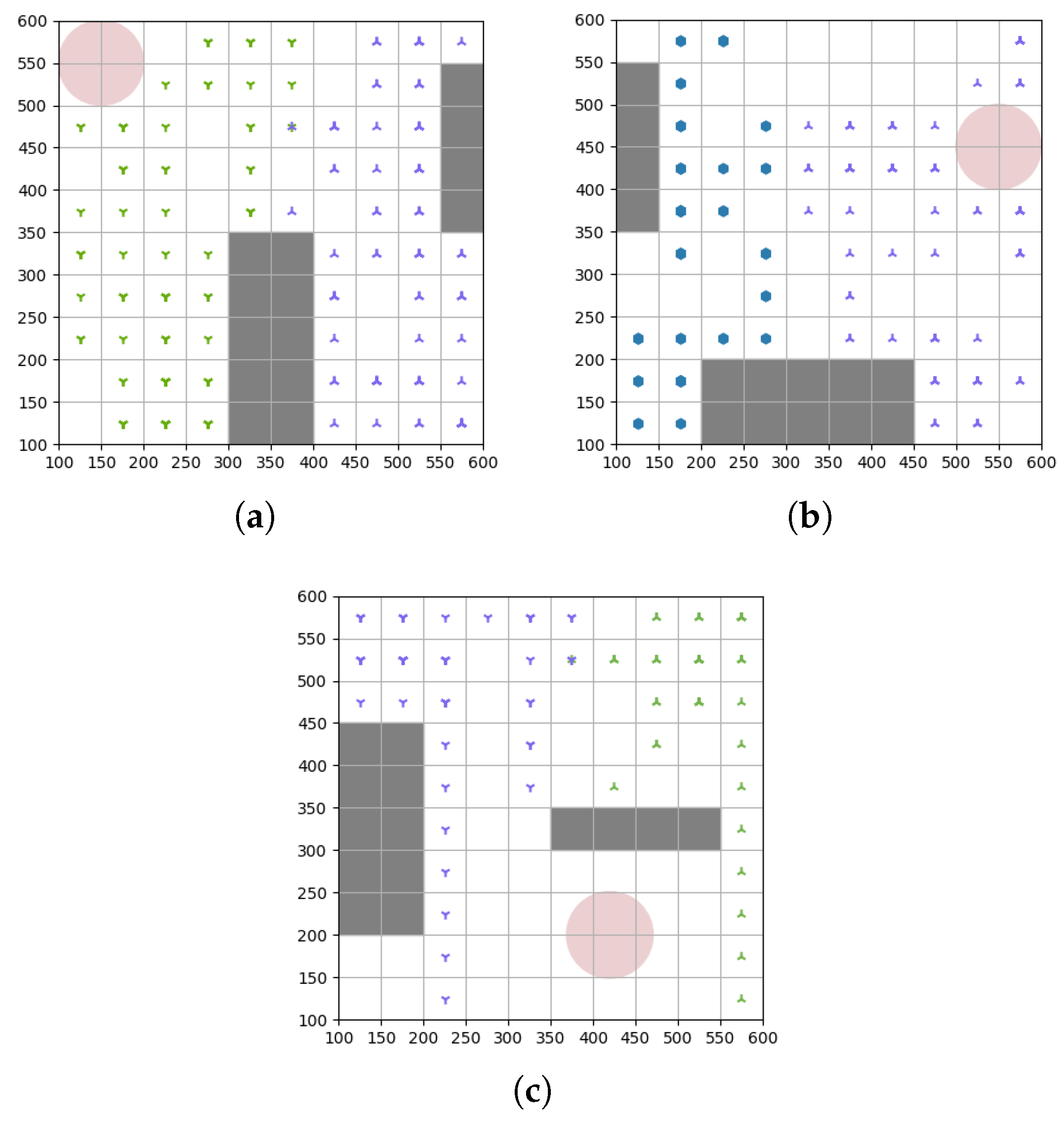
A path-planning method based on a multi-intelligence deep reinforcement learning framework is proposed to maximize the coverage of the target area.

(2)

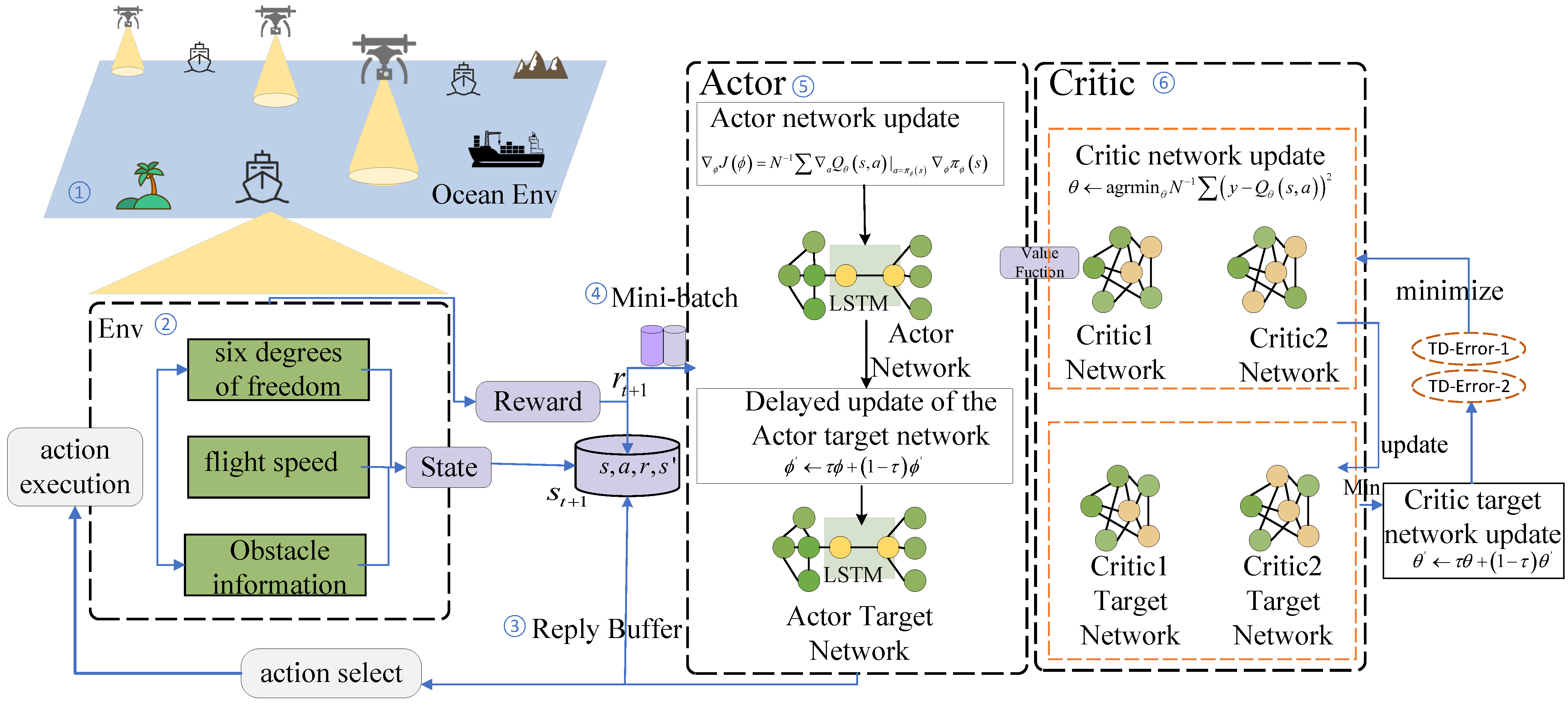
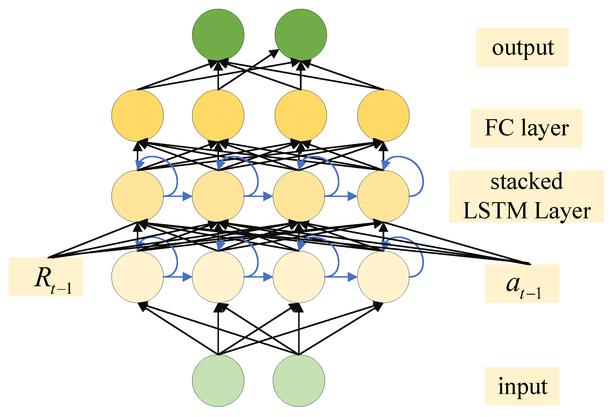
To address the path-planning problem under the condition of partially incomplete information, we utilized an S-LSTM to store and utilize previous states. Furthermore, to address the non-convex problem in optimizing the objective function, we employed multiagent collaboration and experience sharing within the MATD3 algorithm.

(3)

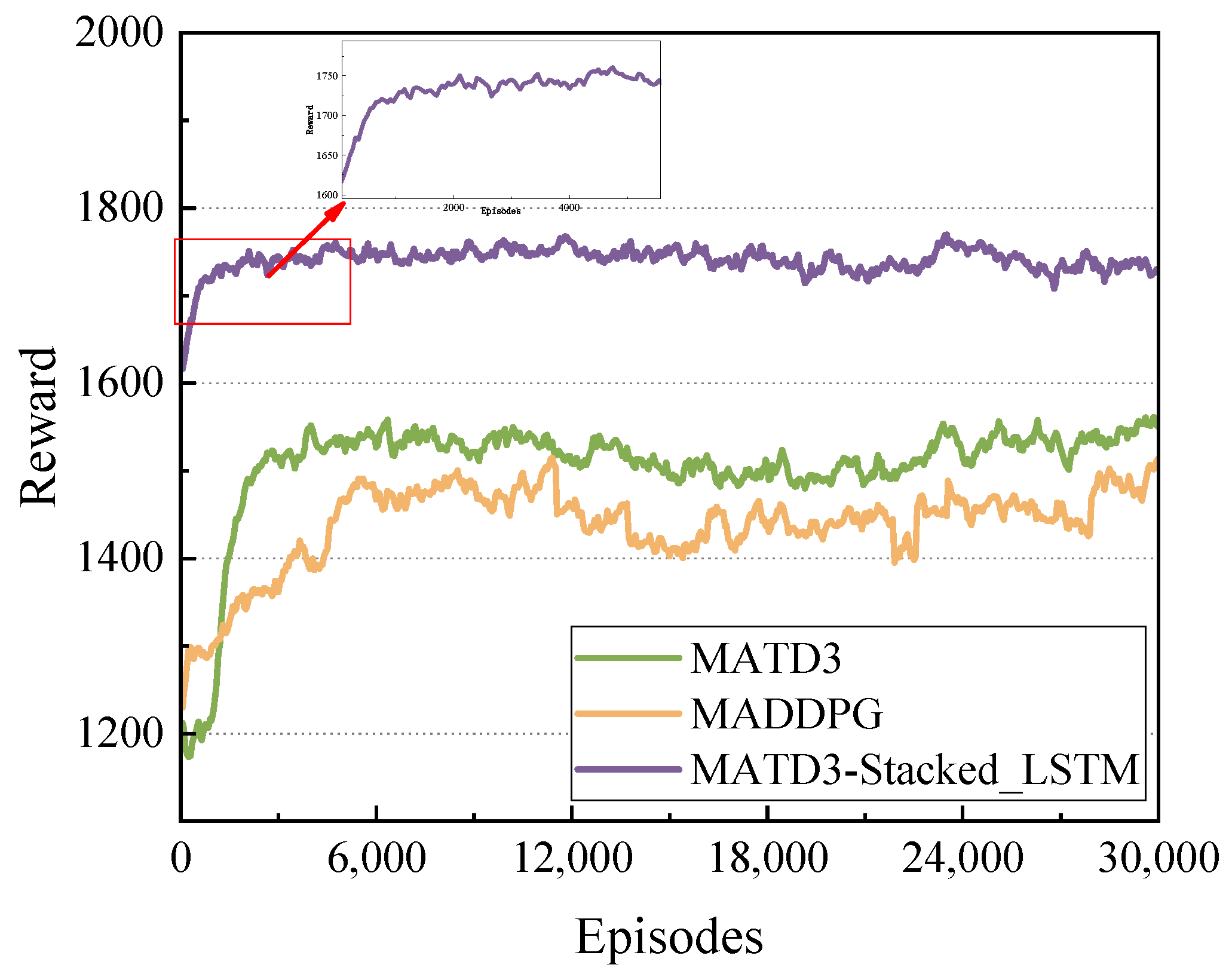
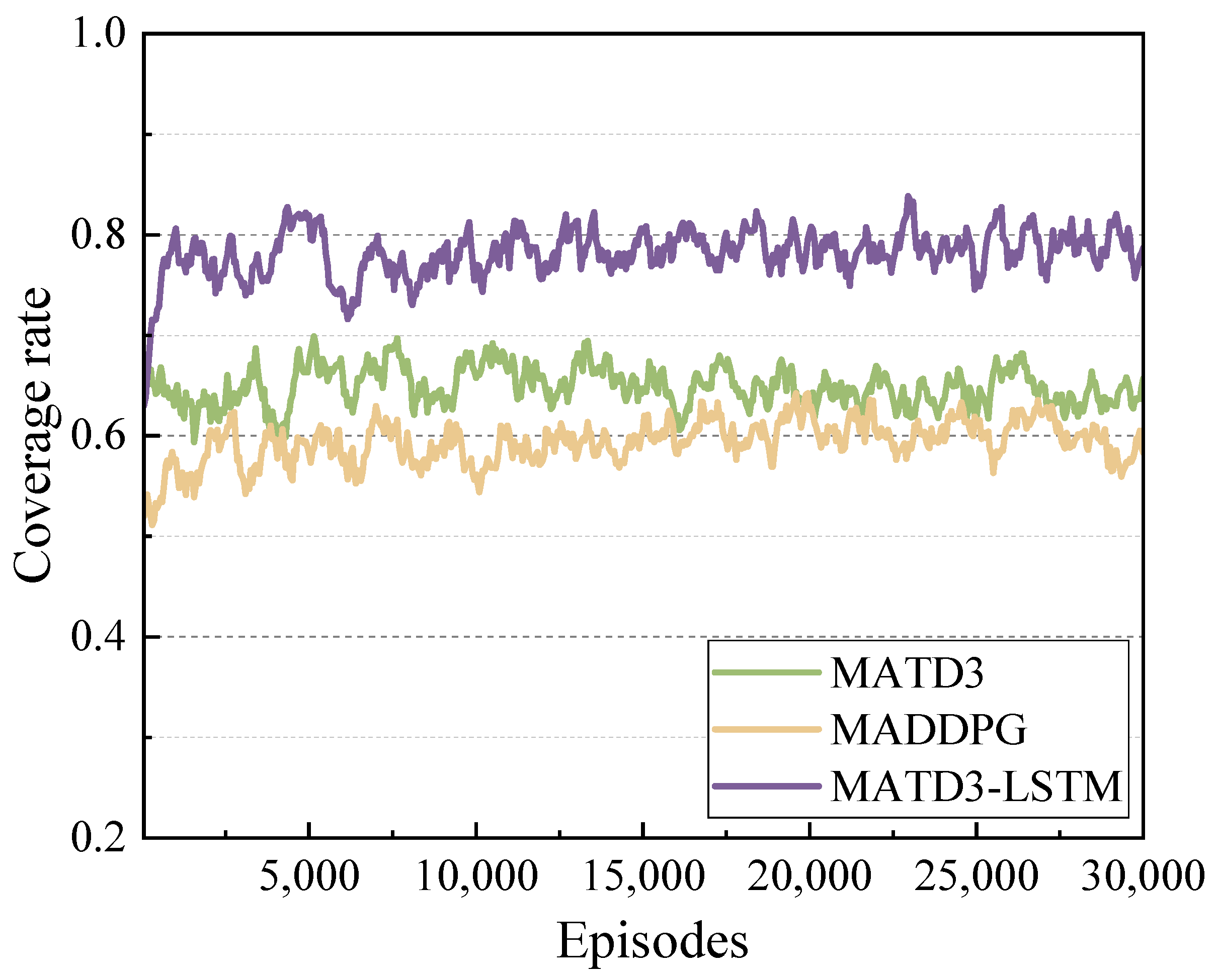
The simulation results demonstrate that the proposed MATD3-Stacked_LSTM algorithm has better convergence and significantly improves the coverage of the target area compared to the other two algorithms.

2. Related Work

Nowadays, heuristic algorithms are widely used for UAV path planning. For instance, Recep Ozdag [13] developed an optimal fitness value search method for continuous and discrete data ranges based on particle swarm optimization (PSO) and electromagnetic-like (EML) algorithms, aiming to ensure the best coverage rate of user devices positioned at certain distance intervals. However, heuristic algorithms require reoptimization and solving when ocean environment data change, making them less adaptive. Additionally, due to inherent algorithmic limitations, they often cannot provide corresponding solutions quickly, making it difficult to adapt to scenarios with high real-time requirements. Therefore, combining cooperative exploration among drones and DRL algorithms can address the challenges posed by the real-world environment. Many existing DRL methods focus only on a single-drone scenario. Bouhamed et al. [14] proposed an autonomous drone path-planning framework using the DDPG method, aimed at training drones to avoid obstacles and reach target points. Li et al. [15] proposed a real-time path-planning approach based on a deep Q network (DQN) to solve the problem of an unknown environment. Unlike quadrotor UAVs, this method provides real-time action planning for fixed-wing UAVs on a feasible path while satisfying the kinematic constraints.

Recently, several works have been proposed to address the problem of path planning using multiple UAVs. Wang et al. [16] proposed a D3QN-based learning method for decision-making policies of typical UAVs, which requires no prior knowledge of the environment (such as channel propagation models and obstacle positions) and other UAVs (such as their tasks, movements, and policies). Numerical results show that real-time navigation can be performed efficiently with high success rates and low collision rates. Liu et al. [17] studied a mobile edge computing network installed on UAVs. They formulated the trajectory optimization problem as a Markov decision process and developed a QoS-based action selection policy based on the DDQN algorithm. DTPC [18] was designed in a multiagent reinforcement learning (MARL) framework based on MADDPG, which solves the problem of decentralized joint trajectory and transmission power control for multi-UAV ABS networks. Harald Bayerlein et al. [19] proposed a novel end-to-end reinforcement learning approach for autonomous trajectory planning of UAVs to collect data from IoT devices in urban environments in support of next-generation communication networks. HAS-DQN [20] is an algorithm that combines the hexagonal area search (HAS) approach with a multiagent DQN. It effectively addresses collision issues among drones by constraining the overall coverage area of the UAVs. Xie et al. [9]. designed a locally optimal UAV path-planning algorithm by leveraging 3D antenna radiation patterns and multistage D3QN. Numerical results substantiate the algorithm’s effectiveness in the context of connectivity-aware UAV path planning.

However, in MARL-based path planning algorithms, each intelligent agent can only observe partial environmental information, overlooking the historical interaction among agents and environmental changes [21]. This may lead to increased difficulties in information propagation and coordination, especially in large-scale multiagent systems. Recurrent Neural networks (RNNs) can memorize and process sequential data [22]. However, RNNs tend to suffer from the vanishing gradient problem, causing them to forget long-term information. LSTM, as a sequence-modeling method, addresses this issue by introducing “forget gates” to improve the RNN structure. Therefore, using MATD3 combined with LSTM can consider the temporal correlations in agent path planning, enabling agents to make decisions with a more long-term planning capability rather than solely focusing on the current state.

3. System Model and Problem Statement

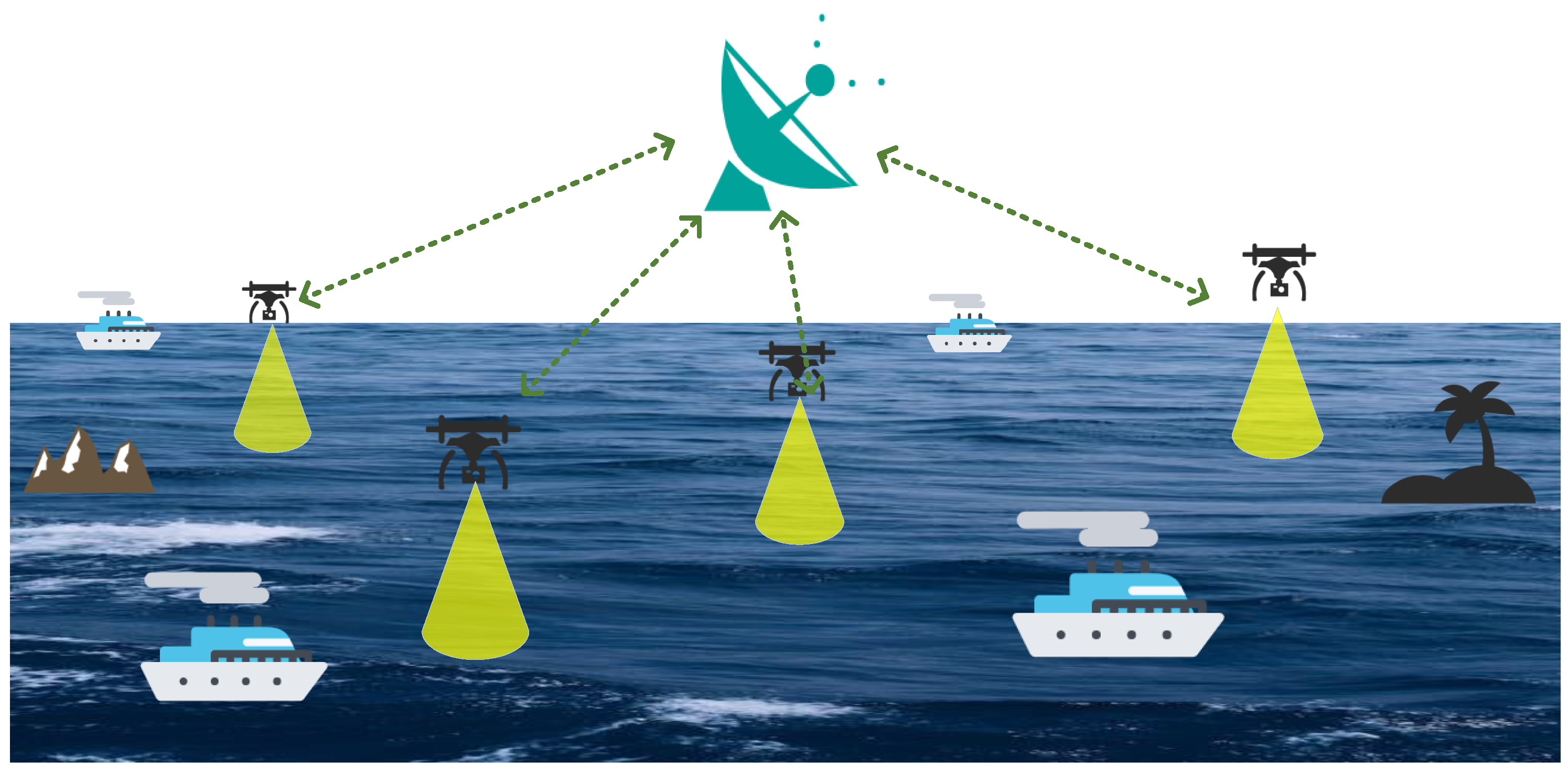
In this study, we propose a multidrone path coverage planning method based on MDRL for data collection in unknown marine environments. In this section, we first introduce the various system models in detail, then formulate the optimization problem for maximization of the coverage rate. We summarize the parameters used in this section in

Table 1. Summary of symbols used in this chapter.

3.1 System Model
m,$\mathcal{M}$	Index, set of UAVs
$t,\mathcal{T}$	Time slot
$(x,y,z),(X,Y,Z)$	Drone coordinates
$\mathbf{P}$	UAV path collection
$\mathbf{F}$	Indicator for UAV trajectory avoiding no-fly zones
$\mathbf{O}$	Indicator for UAV trajectory avoiding obstacles
$\theta$	Flight steering angle
$\left(L_x,L_y\right)$	Shadow area
$\mathcal{B}$	Specified airspace boundary
H	Flying height
$sr$	Spatial resolution
$\mathbf{R}$	Turning radius
$\widehat{\mathcal{D}}$,$\widehat{d}$	Distance between UAVs
V,$\mathcal{A}$	Speed and acceleration
E	Energy consumption of UAVs
C	Battery capacity
$\mathbf{r}$	Battery consumption rate
T	Total time
$\mathcal{A}$	Set of non-obstacle and non-restricted areas
3.2 Problem Formulation
N	The number of grid cells
$\mathbf{A}$	The set of all non-obstacles (non-restricted)

Note: The definitions of notations above apply only to this section.

.

3.1. System Model

3.1.1. UAV Model

Let $\mathcal{M}=\left\{1,2,3,\dots ,M\right\}$ denote the set of UAVs. At each time step (t), the flight direction of UAV $m\in \mathcal{M}$ is determined by the turn angle (${\theta }_{m,t}\in [0,2\pi )$). The flight distance is determined by $d_{m,t}\in [0,d_{max}]$, where $d_{max}$ is the maximum allowed flight distance, and UAVs cannot exceed the boundaries of the target area.

The trajectory of each drone can be represented as:

$${\mathbf{P}}_m=(x_{m,1},y_{m,1},z_{m,1}),(x_{m,2},y_{m,2},z_{m,2}),\dots ,(x_{m,t},y_{m,t},z_{m,t})$$

(1)

where ${\mathbf{P}}_m$ is the trajectory of UAV m, and $(x_{m,t},y_{m,t},z_{m,t})$ represents the position of UAV m at time step t.

When performing coverage tasks, UAVs are not allowed to enter no-fly zones and pass through obstacles. Let $F=\{f_1,f_2,\dots ,f_n\}$ represent the set of no-fly zones and $O=\{o_1,o_2,\dots ,o_k\}$ represent the set of obstacles. The UAV trajectories should avoid crossing F and O.

The constraints can be formulated as follows: The UAV trajectory should not intersect any no-fly zone:

$$\begin{array}{cc}\hfill & (x_{m,i},y_{m,i},z_{m,i}),(x_{m,i+1},y_{m,i+1},z_{m,i+1})\notin \mathbf{F},\hfill \\ \hfill & \forall m\in \mathcal{M},\forall i=1,2,\dots ,t-1\hfill \end{array}$$

(2)

The UAV trajectory should not intersect any obstacle:

$$\begin{array}{cc}\hfill & (x_{m,i},y_{m,i},z_{m,i}),(x_{m,i+1},y_{m,i+1},z_{m,i+1})\notin \mathbf{O},\hfill \\ \hfill & \forall m\in \mathcal{M},\forall i=1,2,\dots ,t-1\hfill \end{array}$$

(3)

where t is the number of time steps taken by UAV m in its trajectory. The notation $(x_{m,i},y_{m,i},z_{m,i})$ represents the position of UAV m at time step i in the 3D space. The constraints ensure that each UAV’s trajectory avoids both the no-fly zones and obstacles during the coverage tasks.

Subsequently, the trajectory of the UAV must not exceed the specified airspace boundary, which is denoted as

$$\mathcal{B}=\{(x_{m,1},y_{m,1},z_{m,1}),(x_{m,2},y_{m,2},z_{m,2}),\dots ,(x_{m,b},y_{m,b},z_{m,b})\}.$$

Each point ($r_i$) in $\mathcal{B}$ represents a 3D coordinate in the airspace. To ensure that the UAV remains within the defined airspace at all times, the position of the UAV at each time step (i) should satisfy the following constraint:

$$(x_i,y_i,z_i)\in \mathcal{B},\forall i=1,2,\dots ,t$$

(4)

This constraint ensures that at each time step, the position of the UAV is within the specified airspace boundary defined by the $\mathcal{B}$ set. It guarantees that the UAV remains within the specified airspace during its entire trajectory.

A UAV flying at a given height (H) from the ground acquires an image corresponding to a specific portion of the area (projected area). The size of the projected area depends on the height (H) and the angle of view ($fOA$). The size of the projected area ($\left(L_x,L_y\right)$) can be calculated as

$$L_x=2H·tan\left(\frac{fOAx}{2}\right)$$

(5)

$$L_y=2H·tan\left(\frac{fOAy}{2}\right).$$

(6)

Therefore, the spacial resolution ($sr$) obtained by taking a picture at height H is

$$sr=\frac{l_x}{L_x}=\frac{l_x}{2H·tan\left(\frac{fOAx}{2}\right),}$$

(7)

where the pixel width of the photo is denoted as $l_x$. Similarly, the formula for calculating the vertical spatial resolution ($R_y$) is given as $l_x/(2\times H\times \tan (fOAy/2))$.

Therefore,

$$H_{min}\le H\le \frac{l_x}{2sr·tan\left(\frac{fOAx}{2}\right)}$$

(8)

where $H_{min}$ is the lower bound for the height of UAVs for safety. Hence, the mission requirement imposes a constraint on the maximum height the UAV can fly, which is

$$H_{max}=\frac{l_x}{2sr·tan\left(\frac{fOA}{2}\right)}$$

(9)

Furthermore, we denote the distance between UAV m and UAV $m^{\prime }$ in t as $D_{m,m^{\prime },t}$, which can be expressed as

$${\mathcal{D}}_{m,m^{\prime },t}=\sqrt{{\left(X_{m,t}-X_{m^{\prime },t}\right)}^2+{\left(Y_{m,t}-Y_{m^{\prime },t}\right)}^2}$$

(10)

We assume that the UAVs should keep a minimal distance of ${\widehat{\mathcal{D}}}_{min}$ to avoiding their collision in each $\mathcal{T}$. Then, we have

$${\mathcal{D}}_{m,m^{\prime },t}\ge {\mathcal{D}}_{min},\forall m,m^{\prime }\in \mathcal{M},m\ne m^{\prime }.$$

(11)

To avoid interference beyond the coverage area, we consider ensuring that the minimum distance between drones is greater than their communication coverage range. Therefore, we introduced communication coverage constraints into path optimization, which can be expressed as:

$$d_{m{m}^{\prime }}>=R_{\mathrm{cov}}$$

(12)

where $d_{m{m}^{\prime }}$ is the communication distance between UAVs m and $m^{\prime }$, and $R_{c}ov$ is the communication coverage radius.

In addition, we can obtain the maximum velocity and maximum acceleration of the UAV.

$$\frac{V_{m,t}-V_{m,t-1}}{\Delta t}<max\left({\mathcal{A}}_m\right)$$

(13)

$$V_{m,t}\le V_{max}$$

(14)

During the execution of a mission, constraints on the turning angles of multiple drones need to be considered. Turning a drone requires both time and space, and excessively large or small turning angles can affect the efficiency of the drone’s path planning and execution. If the turning angle is too large, the drone requires more time and space to complete the turn, which can reduce its execution efficiency. Conversely, if the turning angle is too small, the drone may deviate from the planned path during execution, resulting in flight errors.

$$|{\theta }_m\left(t\right)-{\theta }_m(t-1)|\le \Delta \theta ,\forall m\in \mathcal{M},\forall t\ge 2$$

(15)

where ${\theta }_m\left(t\right)$ represents the heading of the m-th drone at time t, while $\Delta \theta$ denotes the maximum turning angle.

In addition, to ensure that drones do not leave the coverage area when turning and to control the path-planning trajectory of the drones, avoiding excessively complex path planning, constraints on the turning radius need to be considered in multidrone path planning.

$$\left|\left[\begin{array}{cc}cos\left({\theta }_m\left(t\right)\right)& sin\left({\theta }_m\left(t\right)\right)\\ -sin\left({\theta }_m\left(t\right)\right)& cos\left({\theta }_m\left(t\right)\right)\end{array}\right]\left[\begin{array}{c}\Delta x\\ \Delta y\end{array}\right]\right|\ge R,\forall m,t$$

(16)

where $\Delta x$ and $\Delta y$ refer to the difference between the x and y coordinates of the m-th drone between time steps t and $t-1$, ${\theta }_m\left(t\right)$ is the turn angle of the m-th drone at time, R represents the minimum turn radius in drone path planning, and $\left|·\right|$ is the Euclidean paradigm (L2 paradigm) used to compute the length of a vector obtained by matrix–vector multiplication. For vector $(x,y)$, the Euclidean norm is given by $\left|(x,y)\right|=\sqrt{x^2+y^2}$.

3.1.2. Energy Model

During mission execution, each drone has a different battery-life limit. Failure to consider battery-life limits may result in certain drones losing control due to battery depletion during task execution and thus being unable to complete the task, affecting coverage and task performance. Therefore, to ensure that each drone can complete the task and return, constraints on battery-life limits need to be considered.

Taking into account factors such as flight energy consumption and turning energy consumption, we define the energy constraint of each drone as its total energy consumption throughout the flight mission, which cannot exceed its energy capacity. Let the energy capacity of each drone be denoted as C, the energy consumption rate be denoted as $\mathbf{r}$, the total time denoted as T, and the initial energy level denoted as $E_0$. The energy level ($E_t$) of a drone at time t can be calculated using the following equation:

$$E_t=E_0-{\int }_0^t\mathbf{r}∥\frac{dx}{dt}∥dt$$

(17)

where x is the position vector of the drone, $\left|\frac{dx}{dt}\right|$ is the magnitude of the drone’s velocity, and t is the current time.

Therefore, for the power constraint of each UAV can be described using the following formula:

$${\int }_0^T\mathbf{r}∥\frac{dx}{dt}∥dt\le C-E_0$$

(18)

Considering the flight energy consumption, turning energy consumption, and communication energy consumption, let the speed of UAV i be $V_i$ and its flight energy consumption at moment t be $E_i\left(t\right)$; then:

$${\int }_0^{t_f}{E}_m\left(t\right)dt\le E_{m,max}$$

(19)

$${\int }_0^{t_f}{E}_m^{turn}\left(t\right)dt\le E_{m,max}^{turn}$$

(20)

$${\int }_0^{t_f}{E}_{m{m}^{\prime }}^{comm}\left(t\right)dt\le E_{m{m}^{\prime },max}^{comm}$$

(21)

where $t_f$ denotes the moment when the UAV ends its flight, $E_{m,max}$ is the maximum energy consumption of UAV m, $E_{m,max}^{turn}$ is the maximum energy consumption of UAV m for a turn, and $E_{m{m}^{\prime },max}^{comm}$ is the maximum communication energy consumption between UAV m and UAV $m^{\prime }$.

$$E_{m,max}^{turn}+E_{m{m}^{\prime },max}^{comm}+E_{m,max}\le {\int }_0^T\mathbf{r}∥\frac{dx}{dt}∥dt$$

(22)

Therefore, our goal is to find a set of paths ($(x_{m,1},y_{m,1},z_{m,1}),(x_{m,2},y_{m,2},z_{m,2}),\dots ,$$(x_{m,t},y_{m,t},z_{m,t})$) that maximizes the covered area. Specifically, our objective is to maximize the following expression, considering the energy consumption and turn constraints:

$$\frac{1}{N}{\sum }_{i=1}^N\left((x_i,y_i,z_i)\in \mathbf{A}\right)$$

(23)

where N represents the total number of grid cells in the grid environment. The formula for maximizing the coverage rate describes how to evaluate the quality of a set of paths. $\mathbf{A}$ denotes the set of all non-obstacle and non-restricted areas, where $\left(x_i\in A\right)$ is an indicator function that determines whether a path ($x_i$) can cover a non-obstacle and non-restricted area. ${\sum }_{i=1}^N\left(x_i\in \mathbf{A}\right)$ indicates the number of cells that the set of paths ($x_1,x_2,\dots ,x_m$) can cover.

3.2. Problem Formulation

The objective of the optimization problem is to maximize this coverage rate. The coverage path-planning problem consists of one objective function and ten constraint conditions, which represent different aspects of task performance. We formalize the optimization problem as follows:

$$\underset{x_1,x_{2,}\dots ,x_m}{max}\frac{1}{N}{\sum }_{i=1}^N\mathbb{I}\left((x_i,y_i,z_i)\in \mathbf{A}\right)$$

(24)

where $(x_i,y_i,z_i)$ represents the path of the i-th UAV, $\mathbf{A}$ denotes the coverable area, and $\mathbb{I}(x_i\in \mathbf{A})$ indicates whether $x_i$ falls within $\mathbf{A}$.

s. t.:

(1)

$d_{m{m}^{{}^{\prime }}}\ge R_{\mathrm{cov}}\forall m,m^{\prime }\in \mathcal{M},m\ne m^{\prime }$

(2)

$0\le d_{m,t}\le d^{max},\forall m\in \mathcal{M},t\in \mathcal{T}$

(3)

$H_{min}\le H\le \frac{l_x}{2\mathbf{r}·tan\left(\frac{fOAx}{2}\right)}$

(4)

${\mathcal{D}}_{m,m^{\prime },t}\ge {\mathcal{D}}_{min},\forall m,m^{\prime }\in \mathcal{M},m\ne m^{\prime }$

(5)

$\frac{V_{m,t}-V_{m,t-1}}{\Delta t}<max\left({\mathcal{A}}_m\right),\forall m\in \mathcal{M}$

(6)

${\int }_0^t\mathbf{r}∥\frac{dx}{dt}∥dt\le C-E_0$

(7)

$E_{m,max}^{turn}+E_{m{m}^{\prime },max}^{comm}+E_{m,max}\le {\int }_0^T\mathbf{r}∥\frac{dx}{dt}∥dt$

(8)

$|{\theta }_m\left(t\right)-{\theta }_m\left(t-1\right)|\le \Delta \theta ,\forall m\in \mathcal{M},t\in \mathcal{T}$

4. Design

4.1. MATD3

The MADDPG algorithm tends to overestimate Q value, especially during early stages of training [23]. It should be noted that most real-world applications are stochastic, which has been shown to lead to higher value-function overestimation due to added noise from function approximator errors.

The MATD3 algorithm extends TD3 to the multiagent setting in a way similar to how DDPG is extended to MADDPG. This algorithm addresses the stability problem and non-convex optimization objective in collaborative multiagent decision making. It improves upon the DDPG algorithm by optimizing policies, introducing interactions among multiple agents and using double Q networks to evaluate action values. In Figure 2, ⑤ and ⑥ illustrate the update process of the actor and critic networks, respectively.

The Q-function update formula in the MATD3 algorithm is expressed as:

$${\mathcal{L}}_i^Q\left(\theta \right)={\mathbb{E}}_{\left(s,a,r,s^{\prime }\right)\sim U\left(D\right)}\left[{\left(y_i-Q\left(s,a;{\theta }^{-}\right)\right)}^2\right]$$

(25)

where ${\mathcal{L}}_i^Q\left(\theta \right)$ is the loss function of the critic network for agent i with its parameters ($\theta$); ${\mathbb{E}}_{(s,a,r,s^{\prime })\sim U\left(D\right)}$ denotes the expectation over the replay buffer (D) containing samples of state–action–reward–next state tuples; and $y_i$ is the target value for updating the critic, representing the TD target for the MATD3 algorithm.

The TD target ($y_t=r_t+\gamma Q^{\prime }(s_{t+1},{\mu }^{\prime }\left(s_{t+1}\right|{\theta }^{{\mu }^{\prime }})|{\theta }^{Q^{\prime }})$) in the MATD3 algorithm is computed by the target critic network. To enhance exploration and accelerate convergence, a clipped Gaussian noise is introduced for action exploration. Specifically, a noise vector ($ϵ$) is generated based on the deterministic policy ($\mu \left(s\right|{\theta }^{\mu })$), then multiplied by a learnable parameter ($\sigma$) and added to the selected action; that is:

$$a=\mu \left(s\right|{\theta }^{\mu })+ϵ,ϵ\sim \mathbf{N}(0,{\sigma }^2)$$

(26)

Therefore, the noisy Q value can be written as $Q(s_t,a_t|{\theta }^Q)+ϵ$, where ${\theta }^Q$ represents the parameters of the critic network. The clipped Gaussian noise can be bounded using the clip function, restricting it to a certain range, such as $[-c,c]$. Thus, the noisy target ($y_t$) can be expressed as:

$$y_t=r_t+\gamma Q^{\prime }(s_{t+1},{\mu }^{\prime }\left(s_{t+1}\right|{\theta }^{{\mu }^{\prime }})|{\theta }^{Q^{\prime }})+clip\left(ϵ,-c,c\right)$$

(27)

The actor network update in MATD3 is as follows:

$${\nabla }_{{\theta }_i}\mathcal{J}\approx \frac{1}{\mathbf{N}}\sum _j{\nabla }_{{\theta }_i}{Q}_i\left(s,a_i;{\theta }_i\right){|}_{s=s_j,a_i={\mathbf{f}}_i\left({\mathbf{o}}_j;{\theta }_{{\mathbf{f}}_i}\right)}$$

(28)

where $f_i$ represents the actor network of the i-th agent, ${\mathbf{o}}_j$ represents the observation vector of the j-th agent, and $\mathbf{N}$ denotes the number of training samples. ${\nabla }_{{\theta }_i}\mathcal{J}$ is the gradient of the actor network’s objective function for agent i with respect to its parameters (${\theta }_i$). The update is approximated using samples from the replay buffer, where $s_j$ is the state observation of the j-th sample, and ${\mathbf{f}}_i$ is the actor network function for agent i with its parameters (${\theta }_{{\mathbf{f}}_i}$).

The MATD3 algorithm exhibits excellent performance in multiagent cooperation problems, but it has certain limitations when dealing with high-dimensional state spaces, as it cannot fully exploit the dynamic relationships and patterns between state sequences. LSTM neural networks, on the other hand, can capture the dynamic relationships and patterns within state sequences, providing better state representations. Combining MATD3 and LSTM can enable agents to better understand and adapt to changes in the environment, further improving the performance of multiagent systems.

A single LSTM layer consistently underperforms the stacked LSTM structure. To capture the experience gained by UAVs during environmental interactions, we employed a two-layer stacked LSTM network. As illustrated in Figure 3, in the first LSTM layer, the UAV’s position, velocity, and direction serve as inputs. The outputs from this layer, along with the rewards and actions obtained by the UAV in the previous time step, are then fed into the second LSTM layer.

Moreover, LSTM can store and utilize previous states through its memory function, which is beneficial for solving path-planning problems under partially observable conditions. The output of the LSTM is given by:

$$h_t=LSTM\left(s_t,h_{t-1}\right)$$

(29)

where $s_t$ represents the state at time t, and $h_t$ denotes the output state of the LSTM.

Finally, the output of the LSTM is combined with the observation vector in MATD3 to obtain the agent’s state representation:

$$s_t^i=\left[\begin{array}{c}{o}_t^i\\ h_t^i\end{array}\right]$$

(30)

where $o_t^i$ is the observation vector of agent i at time t, and $h_t^i$ is the LSTM output state of agent i at time t.

Thus, as shown in Figure 2, the MATD3-Staked_LSTM algorithm leverages LSTM networks to model state representations, capturing temporal information within time series data, as well as sequential dependencies between UAVs. The agent selects actions through an actor network and incorporates noise upon execution. Subsequently, a batch of data is randomly sampled from the experience replay buffer comprising states, actions, rewards, and next states. A critic network then computes target Q values based on this sampled batch. The TD target is calculated using the target Q values to minimize the loss function, thereby updating the critic network. Concurrently, the actor network parameters are updated through policy gradient estimation based on the sampled policies. Finally, the target networks are softly updated. As presented in Algorithm 1, we can obtain the MATD3-Stacked_LSTM-based path-planning algorithm for multiple UAVs.

Algorithm 1 Multi-UAV coverage path planning based on MATD3-Stacked_LSTM algorithm

1: Initialize critic network parameters ${\theta }_Q$, actor network parameters ${\theta }_{\mu }$, set discount factor $\gamma$, experience replay buffer D 2: for t = 1 to T do 3:    Get the current state $s_t$ representation from LSTM; 4:    Select action $a_i$ 5:    According to the noise ${ϵ}_i\sim \mathcal{N}(0,\sigma )$ get the execution action $a_i\sim \mu \left(s_t\right)+ϵ$, observe the r value 6:    for agent i = 1 to N do 7:        Randomly fetch a batch of data $(s_i,a_i,r_i,s_{i+1})$ from experience playback cache D 8:        Process via LSTM network; 9:        Calculate the target Q value: $Q^{\prime }(s_{i+1},u^{\prime })$ 10:      Calculate TD target: ${\mathbf{y}}_i=r_i+\gamma Q^{\prime }(s_{i+1},u^{\prime }+ϵ)$,where ${ϵ}_i\sim clip\left(\mathbf{N}(0,\sigma )\right)$ 11:      Update critic network by minimizing the loss $L={(y_i-Q(s_i,a_i))}^2$ 12:      Update actor network using the sampled policy gradient:      ${\nabla }_{{\theta }_{\mu }}J\approx \frac{1}{N}{\sum }_{i=1}^N{\nabla }_{a}Q(s_i,a;{\theta }_Q){|}_{a=\mu (s_i;{\theta }_{\mu })}{\nabla }_{{\theta }_{\mu }}\mu (s_i;{\theta }_{\mu })$ 13:      Update target networks:      ${\theta }_{Q^{\prime }}\leftarrow {\theta }_{Q^{\prime }}\tau +{\theta }_{Q^{\prime }}(1-\tau )$      ${\theta }_{{\mu }^{\prime }}\leftarrow {\theta }_{\mu }\tau +{\theta }_{{\mu }^{\prime }}(1-\tau )$ 14:    end for 15: end for

4.2. Markov Decision Process

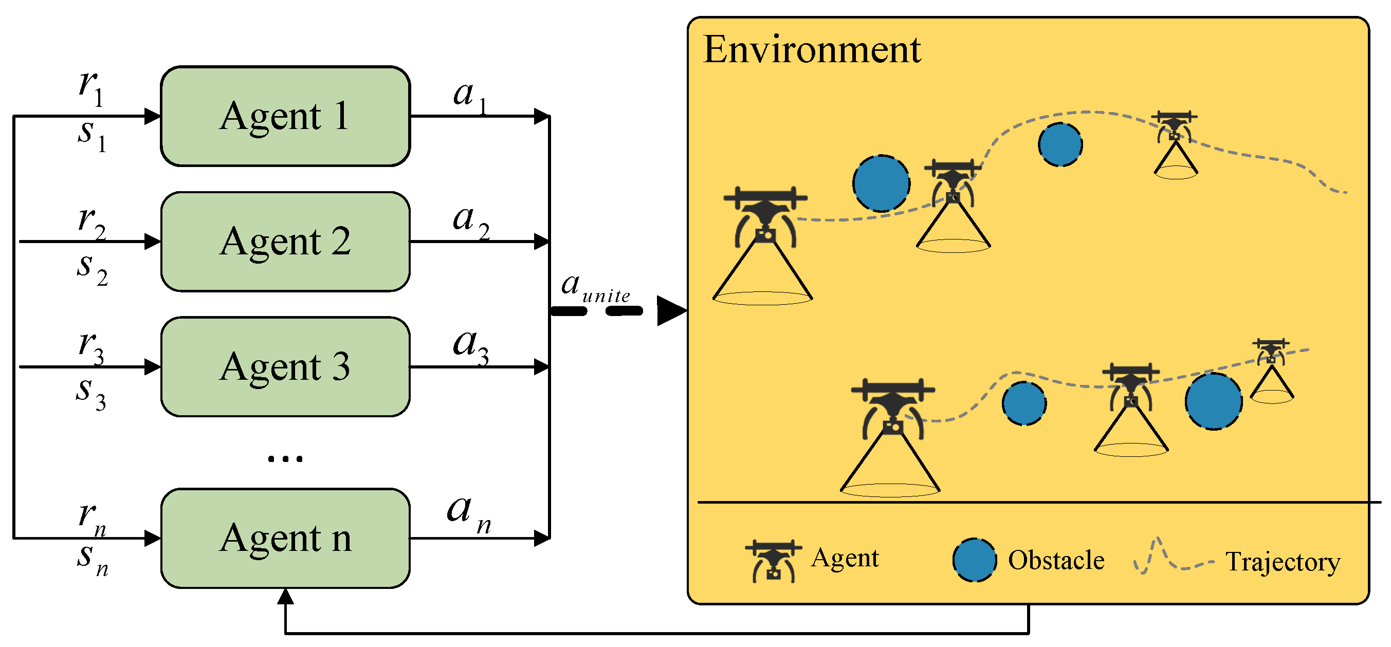
In the MATD3 algorithm, each UAV has its own agent, and they collaborate to accomplish the path-planning task. As shown in Figure 4, each agent receives state information and, based on this information, decides on the next action. We model the UAV path-planning problem as a multiagent reinforcement learning problem, with reinforcement learning model <$S,A,\pi ,R,P$>. Suppose there are m UAVs that need path planning; the state ($s_i$) of each UAV can be represented as its position. Each UAV needs to take an action ($a_i$) to move to the next position. The policy (${\pi }_i$) of each UAV can be represented as a probability distribution mapping the current state to the action space.

4.2.1. Environment

$e_t$ represents the spatial environment where the UAVs are located at time t, including no-fly zones and other obstacles.

4.2.2. State

At each time step (t), the observation state is given as ${\mathbf{o}}_t=[p_t,v_t,d_t]$, where $p_t$, $v_t$, and $d_t$ represent the position, velocity, and direction of the m-th UAV, respectively. The state space is defined as

$$s_t=[{\mathbf{o}}_{t-\widehat{L}+1},\dots ,{\mathbf{o}}_{t-1},{\mathbf{o}}_t]$$

(31)

where $\widehat{L}$ represents the length of the historical state sequence, encompassing the past $\widehat{L}$ states of the i-th drone, leading up to its current state at time step t.

4.2.3. Action

The available actions for all UAVs are $a_t=(a_{1,t},a_{2,t},\dots ,a_{n,t})$, where $a_{i,t}$ represents the actions that the i-th UAV can choose at time step t. $a_t\in A$ represents the actions that the UAVs can perform at time t, including moving east, south, west, and north, as well as and descending.

4.2.4. Reward

In this task, we want agents to cover as much of the map as possible. Therefore, we can use the coverage area of the agents as part of the reward. Specifically, we can evaluate the performance of the agents by calculating the number of grid cells covered by the agents on the map. Then, we can divide this number by the total number of grid cells to obtain a coverage rate. This coverage rate is the value of the reward and can be represented as:

$$r_{rew}=\frac{1}{N}{\sum }_{i=1}^N\left[{\rho }_i==1\right]$$

(32)

where N is the total number of grid cells on the map, ${\gamma }_i==1$ is the i-th grid cell covered by the agents, and $[{\rho }_i==1]$ is an indicator function, taking the value of 1 when ${\rho }_i==1$ and 0 otherwise. If an agent collides with another agent or an obstacle or flies into a no-fly zone, it is penalized. Thus, we can add the penalty value for such situations to the reward value to obtain the final reward value. The penalty value can be represented as:

$$r_{pun}=\left\{\begin{array}{c}-1,\mathrm{collide}\mathrm{or}\mathrm{in}\mathrm{no}\mathrm{flyzone}\hfill \\ 0,\mathrm{otherwise}\hfill \end{array}\right.$$

(33)

To ensure that UAVs can work continuously during the mission, the UAV’s energy consumption needs to be considered. We can use the energy consumption of the UAV as part of the reward and encourage agents to plan their paths efficiently by limiting the UAV’s energy consumption.

$$r_{pun}=\left\{\begin{array}{c}-k_{energy}·E_t,E_t>E_c\hfill \\ c_{energy},E_t\le E_c\hfill \end{array}\right.$$

(34)

where $E_t$ represents the current energy consumption value of the UAV, and $E_c$ represents the upper limit of the UAV’s energy consumption. When the current energy consumption value ($E_t$) exceeds the energy consumption limit ($E_c$), the reward value corresponding to the reward function is $-k_{energy}·E_t$, where $k_{energy}$ is a positive number representing the penalty coefficient for energy consumption. When the energy consumption of the UAV is less than or equal to the energy consumption limit ($E_c$), the reward value corresponding to the reward function is $c_{energy}$, where $c_{energy}$ is a positive number representing the additional reward value after the energy consumption reaches the limit, aiming to encourage agents to better control the energy consumption of the UAV.

The final reward value is the sum of the reward part and the penalty part:

$$rewar{d}_n=r_{rew}+r_{pun}$$

(35)

5. Numerical Result

The task studied in this paper is multi-UAV path planning based on ocean monitoring. In this scenario, the UAVs need to detect and cover targets within a rectangular area in the ocean. There exist unknown obstacles in the area (e.g., sudden emergence of a ship or other UAVs used for detection). Therefore, the UAVs need to autonomously avoid obstacles while detecting the target points. As the target points are all in the ocean area, the scenario can be simplified to a two-dimensional plane.

5.1. Simulation Settings

We constructed a simulated scenario involving multiple UAVs performing coverage tasks. The map size was assumed to be $10\times 10$, with each grid cell having a size of $1\times 1$, amounting to a total of 100 grid cells. The simulation environment was set up using Python 3.6 and PyCharm, with the deep learning library implemented in PyTorch. The initial UAV positions were initialized randomly, and initial actions were randomly selected. The training loop was then executed using the hyperparameters listed in

Table 2. Summary of notations used in the paper.

Notation	Definition
Actor learning rate	1 × 10${}^{-6}$
Critic learning rate	1 × 10${}^{-3}$
$\gamma$	0.95
$\tau$	1 × 10${}^{-5}$
Memory capacity	100,000
Batch size	512
Policy noise	0.6
Noise clip	0.5
Policy delay	2

. At each iteration, experiences were sampled from memory to update the networks. The current policy was evaluated after completing each round of updates. The scenario simulation, algorithm implementation, initialization of parameters, and training procedure helped validate the effectiveness of the proposed MATD3 approach for multi-UAV coverage path planning in a systematic manner.

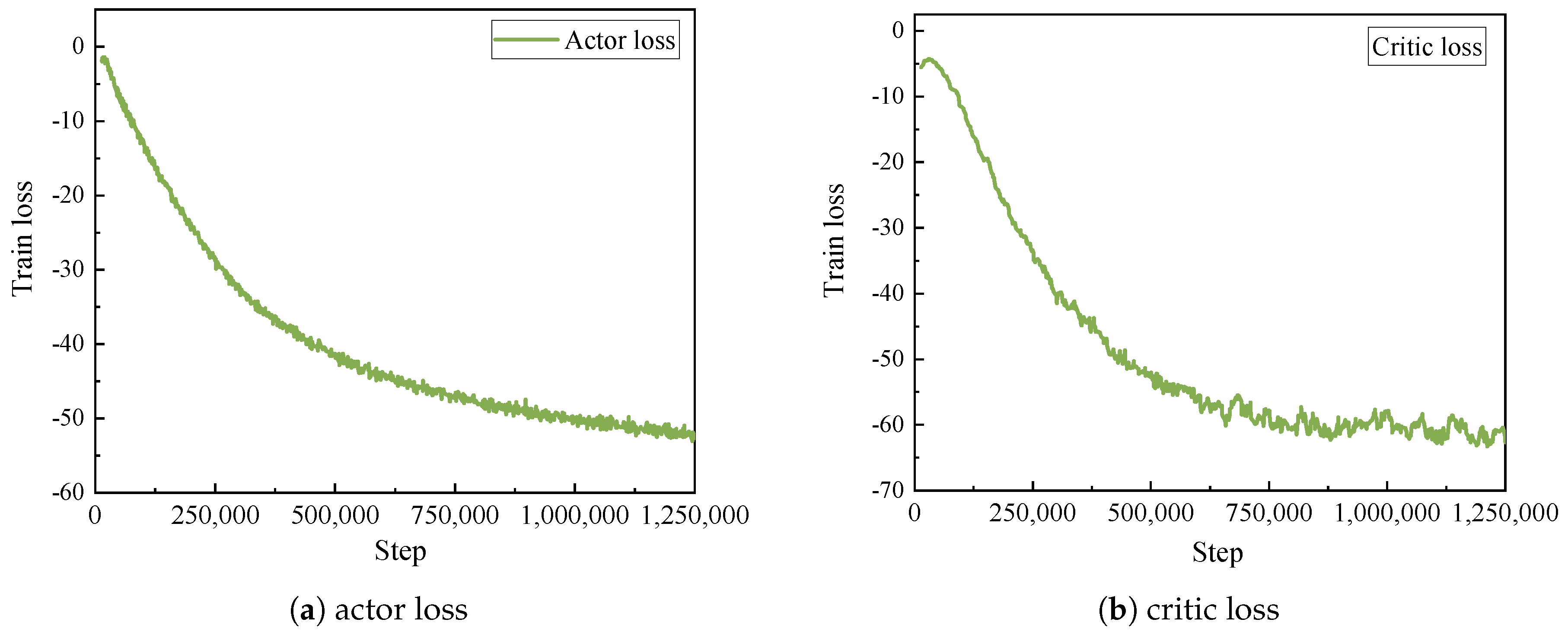
5.2. Convergence Analysis

We compared the performance of three algorithms: MATD3, MADDPG, and our proposed MATD3-Stacked_LSTM. A scenario with four UAVs was used for evaluation. As shown in Figure 5, the reward curves of MATD3 and MADDPG gradually increased and stabilized over training, but MADDPG required about 10,000 episodes to converge, while MATD3-Stacked_LSTM achieved convergence within around 5000 episodes and attained higher final rewards. This suggests that MATD3-Stacked_LSTM outperforms the other two algorithms in terms of faster convergence and superior performance. This superior performance of MATD3-Stacked_LSTM can be attributed to its use of an RNN-based LSTM network for the modeling of joint state representations. LSTM excels at capturing temporal dependencies, and in this multiagent task with long-term dependencies, the LSTM network can more comprehensively learn complex interactions among agents, leading to enhanced state representations.

As shown in Figure 6, the loss values of both the actor and critic networks decrease significantly at the beginning of the training, and the decrease rate gradually slows down with the increase in training steps, eventually approaching stability. This indicates that the MATD3-Stacked_LSTM model gradually learns the optimal policy and value function during the training process and converges to the optimal solution. This also proves the effectiveness and reliability of the model.

The primary requirement of this coverage task is to cover all areas except for obstacles and no-fly zones; hence, the coverage rate is the most important metric. The coverage rate is calculated as the number of covered cells divided by the total number of cells, that is:

$$Cover=\frac{{\displaystyle \sum _{i=1}^m}{\displaystyle \sum _{j=1}^n}Area\left(i,j\right)}{m\times n}$$

(36)

where m and n are the numbers of rows and columns of the map, respectively; $Area(i,j)$ is the coverage status at the ith row and jth column and takes a value of 0 or 1; 1 means covered; and 0 means not covered. The range of the summation is all positions of the whole map. In this experiment, we found:

$$\frac{{\displaystyle \sum _{i,j}}[Are{a}_{i,j}==1]}{100}$$

(37)

where 100 represents the total number of grids.

As shown in Figure 7, the coverage rates obtained by the three algorithms increase rapidly with the increase in the number of episodes, indicating that the three algorithms can quickly adapt to the task environment and gradually improve their exploration and exploitation abilities. MATD3-Stacked_LSTM models temporal dependencies in states using an LSTM network. At each time step, it aggregates observations across agents to learn coordinated joint actions. MATD3 directly operates on raw states without modeling interdependencies. MADDPG extends the single-agent DDPG to a multiagent setting but does not explicitly consider interactions between agents. The coverage rates based on the MATD3-Stacked_LSTM and MATD3 algorithms reach around 80% and 70%, respectively, while the MADDPG algorithm can only reach 60%. This underscores the benefits of explicitly incorporating temporal modeling capabilities via LSTM. It should be noted that since the no-fly zone and obstacles are not coverable, these areas need to be excluded when calculating the coverage rate, so the coverage rate cannot reach 100%.

In order to achieve collaborative data monitoring in a target area using multiple UAVs, we conducted trajectory planning for the UAVs. Figure 8 and Figure 9 show the trajectory maps for two and four UAVs, respectively, completing the coverage task in a 10 × 10 discrete environment. Each UAV cooperatively covers a specific area and avoids obstacles and no-fly zones to maximize the defined reward. As depicted in Figure 9, for the scenario with two drones, the coverage rate of the MATD3-Stacked LSTM algorithm is approximately 65%, which is significantly higher than the other two algorithms. All three algorithms effectively mitigate path overlap. Furthermore, as shown in Figure 9, when deploying four UAVs, their paths overlap, but they can still avoid obstacles and no-fly zones well. Obviously, the MATD3-Stacked_LSTM algorithm covers more cells with lower overlap rates, as shown in Figure 9a. Although the other two algorithms also cover most of the areas, there are higher coverage overlap rates. This indicates that the MATD3-Stacked_LSTM algorithm can better coordinate the decision making of multiple UAVs, thereby achieving more efficient path planning.

The coverage of certain areas may have some degree of overlap, as shown in Figure 10. Therefore, we compared the coverage overlap rate of the three algorithms in multi-UAV coverage tasks. From Figure 10, it can be seen that as the number of UAVs increases, the coverage overlap rate based on the MATD3-Stacked_LSTM algorithm becomes lower than that of the other two algorithms. For example, when the number of UAVs is 4, the coverage redundancy of MATD3-Stacked_LSTM is approximately 9.563, while the other two algorithms have redundancy rates of about 11.754 and 15.654, respectively. This represents a reduction of 18.61% compared to MATD3 and 38.91% compared to MADDPG. The results demonstrate that for multi-UAV coverage tasks, the MATD3-Stacked LSTM algorithm is more suitable for reducing overlap between UAV paths, thereby improving the efficiency and effectiveness of the overall coverage mission compared to MADDPG and MATD3. By modeling temporal dependencies, the LSTM network enables the MATD3-Stacked_LSTM approach to learn coordinated policies that achieve higher coverage rates with less redundancy during multi-UAV path planning.

6. Conclusions

In this paper, we propose an improved MATD3 algorithm with an LSTM model incorporated into the MATD3 model to address the coverage problem of UAVs in the context of ocean data monitoring. The LSTM model is used to consider time series information during the UAV path-planning process. Through comparative experiments between the three algorithms, we have demonstrated that the improved MATD3 algorithm can effectively reduce the redundancy of coverage while ensuring high coverage rates of the target area. Future work can explore online reinforcement learning methods and multiagent communication mechanisms to continuously adapt to dynamic environments during execution. This will advance the applications of drone technology in various real-world settings, making a substantial contribution to the broader field of autonomous navigation systems.

References

1. Yang, F.; Wang, P.; Zhang, Y.; Zheng, L.; Lu, J. Survey of swarm intelligence optimization algorithms. In Proceedings of the 2017 IEEE International Conference on Unmanned Systems (ICUS), Beijing, China, 27–29 October 2017; pp. 544–549. [Google Scholar] [CrossRef]
2. Chang, S.Y.; Park, K.; Kim, J.; Kim, J. Securing UAV Flying Base Station for Mobile Networking: A Review. Future Internet 2023, 15, 176. [Google Scholar] [CrossRef]
3. Li, H.; Wu, S.; Jiao, J.; Lin, X.H.; Zhang, N.; Zhang, Q. Energy-Efficient Task Offloading of Edge-Aided Maritime UAV Systems. IEEE Trans. Veh. Technol. 2022, 72, 1116–1126. [Google Scholar] [CrossRef]
4. Ma, M.; Wang, Z. Distributed Offloading for Multi-UAV Swarms in MEC-Assisted 5G Heterogeneous Networks. Drones 2023, 7, 226. [Google Scholar] [CrossRef]
5. Dai, Z.; Xu, G.; Liu, Z.; Ge, J.; Wang, W. Energy saving strategy of uav in mec based on deep reinforcement learning. Future Internet 2022, 14, 226. [Google Scholar] [CrossRef]
6. Jiang, Y.; Ma, Y.; Liu, J.; Hu, L.; Chen, M.; Humar, I. MER-WearNet: Medical-Emergency Response Wearable Networking Powered by UAV-Assisted Computing Offloading and WPT. IEEE Trans. Netw. Sci. Eng. 2022, 9, 299–309. [Google Scholar] [CrossRef]
7. Savkin, A.V.; Huang, C.; Ni, W. Joint multi-UAV path planning and LoS communication for mobile-edge computing in IoT networks with RISs. IEEE Internet Things J. 2022, 10, 2720–2727. [Google Scholar] [CrossRef]
8. Aggarwal, S.; Kumar, N. Path planning techniques for unmanned aerial vehicles: A review, solutions, and challenges. Comput. Commun. 2020, 149, 270–299. [Google Scholar] [CrossRef]
9. Xie, H.; Yang, D.; Xiao, L.; Lyu, J. Connectivity-Aware 3D UAV Path Design with Deep Reinforcement Learning. IEEE Trans. Veh. Technol. 2021, 70, 13022–13034. [Google Scholar] [CrossRef]
10. Qiming, Z.; Husheng, W.; Zhaowang, F. A review of intelligent optimization algorithm applied to unmanned aerial vehicle swarm search task. In Proceedings of the 2021 11th International Conference on Information Science and Technology (ICIST), Chengdu, China, 21–23 May 2021; pp. 383–393. [Google Scholar] [CrossRef]
11. Gao, S.; Wang, Y.; Feng, N.; Wei, Z.; Zhao, J. Deep Reinforcement Learning-Based Video Offloading and Resource Allocation in NOMA-Enabled Networks. Future Internet 2023, 15, 184. [Google Scholar] [CrossRef]
12. Nguyen, T.T.; Nguyen, N.D.; Nahavandi, S. Deep reinforcement learning for multiagent systems: A review of challenges, solutions, and applications. IEEE Trans. Cybern. 2020, 50, 3826–3839. [Google Scholar] [CrossRef] [PubMed]
13. Ozdag, R. Multi-metric optimization with a new metaheuristic approach developed for 3D deployment of multiple drone-BSs. Peer-Peer Netw. Appl. 2022, 15, 1535–1561. [Google Scholar] [CrossRef]
14. Bouhamed, O.; Ghazzai, H.; Besbes, H.; Massoud, Y. Autonomous UAV Navigation: A DDPG-Based Deep Reinforcement Learning Approach. In Proceedings of the 2020 IEEE International Symposium on Circuits and Systems (ISCAS), Sevilla, Spain, 10–21 October 2020; pp. 1–5. [Google Scholar] [CrossRef]
15. Li, J.; Liu, Y. Deep Reinforcement Learning based Adaptive Real-Time Path Planning for UAV. In Proceedings of the 2021 8th International Conference on Dependable Systems and Their Applications (DSA), Yinchuan, China, 11–12 September 2021; pp. 522–530. [Google Scholar]
16. Wang, X.; Gursoy, M.C.; Erpek, T.; Sagduyu, Y.E. Learning-Based UAV Path Planning for Data Collection with Integrated Collision Avoidance. IEEE Internet Things J. 2022, 9, 16663–16676. [Google Scholar] [CrossRef]
17. Liu, Q.; Shi, L.; Sun, L.; Li, J.; Ding, M.; Shu, F. Path planning for UAV-mounted mobile edge computing with deep reinforcement learning. IEEE Trans. Veh. Technol. 2020, 69, 5723–5728. [Google Scholar] [CrossRef]
18. Chen, B.; Liu, D.; Hanzo, L. Decentralized Trajectory and Power Control Based on Multi-Agent Deep Reinforcement Learning in UAV Networks. In Proceedings of the ICC 2022—IEEE International Conference on Communications, Seoul, Republic of Korea, 16–20 May 2022; pp. 3983–3988. [Google Scholar] [CrossRef]
19. Bayerlein, H.; Theile, M.; Caccamo, M.; Gesbert, D. UAV Path Planning for Wireless Data Harvesting: A Deep Reinforcement Learning Approach. In Proceedings of the GLOBECOM 2020—2020 IEEE Global Communications Conference, Taipei, China, 7–11 December 2020; pp. 1–6. [Google Scholar] [CrossRef]
20. Zhu, X.; Wang, L.; Li, Y.; Song, S.; Ma, S.; Yang, F.; Zhai, L. Path planning of multi-UAVs based on deep Q-network for energy-efficient data collection in UAVs-assisted IoT. Veh. Commun. 2022, 36, 100491. [Google Scholar] [CrossRef]
21. Prédhumeau, M.; Mancheva, L.; Dugdale, J.; Spalanzani, A. Agent-based modeling for predicting pedestrian trajectories around an autonomous vehicle. J. Artif. Intell. Res. 2022, 73, 1385–1433. [Google Scholar] [CrossRef]
22. Wen, G.; Qin, J.; Fu, X.; Yu, W. DLSTM: Distributed Long Short-Term Memory Neural Networks for the Internet of Things. IEEE Trans. Netw. Sci. Eng. 2022, 9, 111–120. [Google Scholar] [CrossRef]
23. Ackermann, J.; Gabler, V.; Osa, T.; Sugiyama, M. Reducing Overestimation Bias in Multi-Agent Domains Using Double Centralized Critics. arXiv 2019, arXiv:1910.01465. [Google Scholar]
Figure 1. Multi-UAVs perform marine data-monitoring missions in target areas.
Futureinternet 15 00369 g001
Figure 2. A framework diagram based on MATD3-Stacked_LSTM for the implementation of multi-UAV coverage planning.
Futureinternet 15 00369 g002
Figure 3. Stacked LSTM structure.
Futureinternet 15 00369 g003
Figure 4. Autonomous decision making for UAVs based on the MATD3 algorithm.
Futureinternet 15 00369 g004
Figure 5. Average reward trends with training episodes (smooth = 0.85).
Futureinternet 15 00369 g005
Figure 6. Average loss trends with training steps (smooth = 0.85).
Futureinternet 15 00369 g006
Figure 7. The changing trend of the coverage of the three algorithms (four UAVs).
Futureinternet 15 00369 g007
Figure 8. The coverage area of two UAVs under different algorithms. The circles are obstacles, and the rectangles are no-fly zones. Both are randomly generated. (a) Coverage area of two UAVs based on the MATD3-Stacked_LSTM algorithm. (b) Coverage area of two drones based on the MATD3 algorithm. (c) Coverage area of two drones based on the MADDPG algorithm.
Futureinternet 15 00369 g008
Figure 9. The coverage area of four UAVs under different algorithms. The circles are obstacles, and the rectangles are no-fly zones. Both are randomly generated. (a) Coverage area of four UAVs based on the MATD3-Stacked_LSTM algorithm. (b) Coverage area of four drones based on the MATD3 algorithm. (c) Coverage area of four drones based on the MADDPG algorithm.
Futureinternet 15 00369 g009
Figure 10. Repeated coverage of three algorithms with different numbers of UAVs.
Futureinternet 15 00369 g010