Multifractal Cross-Correlations of Bitcoin and Ether Trading Characteristics in the Post-COVID-19 Time

Abstract

Unlike price fluctuations, the temporal structure of cryptocurrency trading has seldom been a subject of systematic study. In order to fill this gap, we analyse detrended correlations of the price returns, the average number of trades in time unit, and the traded volume based on high-frequency data representing two major cryptocurrencies: bitcoin and ether. We apply the multifractal detrended cross-correlation analysis, which is considered the most reliable method for identifying nonlinear correlations in time series. We find that all the quantities considered in our study show an unambiguous multifractal structure from both the univariate (auto-correlation) and bivariate (cross-correlation) perspectives. We looked at the bitcoin–ether cross-correlations in simultaneously recorded signals, as well as in time-lagged signals, in which a time series for one of the cryptocurrencies is shifted with respect to the other. Such a shift suppresses the cross-correlations partially for short time scales, but does not remove them completely. We did not observe any qualitative asymmetry in the results for the two choices of a leading asset. The cross-correlations for the simultaneous and lagged time series became the same in magnitude for the sufficiently long scales.

1. Introduction

The cryptocurrency market has once again become the media spotlight during a series of spectacular crashes that have driven bitcoin and other principal cryptocurrencies to lose 75–80% of their market value over roughly half a year until mid-2022, proving that the preceding substantial growths were merely yet another speculation bubble, resembling those that occurred in 2011, 2013, and 2017 [1]. This bubble overlapped with the later part of the COVID-19 pandemic [2,3,4,5,6], raising the question of possible relations between the two, and opened an interesting topic for future research. It has been shown that the pandemic outbreak in early 2020 had some limited effect on the multifractal properties of the price returns [7]. The most important observation is that the cryptocurrencies during the outburst lost their potential to be a safe haven, because they started to be strongly cross-correlated with the regular markets [8,9]. The strength of these correlations has varied with time, but despite the fact that there were periods in which the cryptocurrency market used to evolve rather independently in the post-COVID-19 time [9,10,11,12,13], the overall picture favours strong cross-correlations, especially since Fall 2021. By the post-COVID-19 time, we mean a period after the initial pandemic-related panic had simmered down and the markets started to see the pandemic as a part of daily life, i.e., starting from approximately late Spring 2020. Despite the turbulence that the cryptocurrency market has been coping with since the pandemic outbreak, there are studies suggesting that it has finally reached maturity and, at least from some perspectives, it shows features that are the same as their counterparts in the classic markets [14,15].

Bitcoin (BTC) was introduced in 2009 as the first asset entirely based on the then newly introduced blockchain technology [16]. Its purpose was to provide a decentralised and non-inflationary alternative for fiat currencies, which were subject to massive quantitative easing related to the central bank policies aimed at fighting the consequences of the global financial crisis of 2008–2010. In the beginning, bitcoin was viewed just as a curiosity, even though a transaction that set the bitcoin price expressed in US dollars for the first time took place as early as May 2010, and the first platform designed for cryptocurrency trading was opened in July 2010 [17]. Soon, the investors found that BTC and other cryptocurrencies, which started to emerge after the idea of decentralised finance gained initial recognition, can be used as speculative assets [18]. The first bubble and a subsequent price drop occurred in 2011, when the market was in its infancy, while the subsequent bubbles in 2013 and 2017 appeared at later stages of the cryptocurrency market development [14]. This development is characterised, from a statistical point of view, by a gradual transition from rather idiosyncratic properties of the fluctuation probability distribution functions (pdfs), temporal correlations, and scaling behaviour towards the appearance of the financial stylised facts that are observed in the standard markets [14].

Nowadays, after 12 years of the existence of this market and an enormous variety of assets traded there, the cryptocurrencies have not yet managed to achieve the initial goal envisaged by their founders. Perhaps the most serious issue that prevents them from being considered as a substitute for fiat currencies is their extreme volatility, which attracts large amounts of speculative capital, which in turn amplifies price fluctuations. Volatility is one of the standard indicators of asset liquidity: for a liquid asset, even a large order does not have any significant impact on its price. However, even the most capitalised cryptocurrencies, such as BTC or ether, (ETH) suffer heavily from large price jumps triggered by large orders. This is related, in part, to a much smaller trading frequency on various exchanges compared to the stock and foreign currency markets [19,20]. Interestingly, this important indicator has seldom been the subject of quantitative studies based on tick-by-tick data. Only recently has progress in this direction been reported in Ref. [21], where the inter-transaction times, the number of transactions in unit time, and the traded volume have been analysed. Data representing major cryptocurrencies collected from a few trading platforms have shown that the inter-transaction times are long-term autocorrelated with a power-law decay [21] exactly the same as the data from the regular stock and Forex markets [22,23,24,25,26]. This provides space for future application and testing of relevant stochastic models, such as the Markov switching multifractal duration model [26,27] and the continuous-time random walk model [28,29,30,31] to the cryptocurrency market data. As the inter-transaction times are directly related to the number of transactions in time unit, the latter quantity was also demonstrated to show long-range power-law autocorrelation [32].

The inter-transaction times and the number of transactions in the stock markets were reported to be multifractal [23,33], and the same was observed for the cryptocurrency market data [21]. Multiscaling of the related time series has also been reported, with a strong indication that small fluctuations, i.e., the periods of increased trading frequency, show richer multifractality compared to the large fluctuations associated with the periods of less frequent trading [21]. Slower trading thus happens to be more uncorrelated (efficient) than trading associated with a market frenzy. The long-term autocorrelations of inter-transaction times are also responsible for their distribution tail behaviour, which according to the Ref. [21] cannot be approximated by an exponentially decaying function but, contrastingly, in many cases can be approximated by stretched exponential or power-law functions.

In the present work, we study data that represent a few quantities that characterise the trading of two major cryptocurrencies: BTC and ETH. These quantities are: the logarithmic price returns, the volume traded in time unit, and the number of transactions in time unit. We investigate the fractal properties of these data both from the univariate perspective, in which the properties of each signal are analysed separately, and from the bivariate perspective, in which we look at the cross-correlations between the respective time series of BTC and ETH. As a particularly novel element, we also study the lagged cross-correlations between these assets and seek a possible asymmetry between BTC→ETH and ETH→BTC directions. Our goal is to answer the following questions:

• Do the price returns, the volume, and the number of transactions in the time unit representing the principal cryptocurrencies show any statistical inter-currency cross-correlations that can be detected with the q-dependent detrended cross-correlation coefficient (defined in Section 2)?
• Are those cross-correlations, if present, fractal? That is, does the covariance of the fluctuations of these quantities reveal multiscaling/multifractality over a range of scales?
• Do the cross-correlations, if present, survive if the studied signals have been shifted in time with respect to each other?
• If so, is it possible to observe any asymmetry between the results with respect to a shift direction (BTC→ETH and ETH→BTC)?
• What is a proposed explanation for the outcomes?

Our paper is organised as follows. In Section 2, we present the data on which our study is based, together with the applied multifractal formalism. In Section 3 we report details of the results, and in Section 4, we sum up the results and discuss their implications.

2. Materials and Methods

In this study, we analyse high-frequency data collected from Binance [34], which is the largest cryptocurrency trading platform in terms of daily volume [35]. We analyse time series representing the number of transactions in time unit $N\left(t_i\right)$, logarithmic price returns $r\left(t_i\right)$, and volume traded in time unit $V\left(t_i\right)$ for two major cryptocurrencies: BTC and ETH, which were sampled every $\Delta t=10$ s with $\Delta t=t_{i+1}-t_i$ and $i=1,\dots ,T$. Since cryptocurrency trading is continuous 24/7, our time series that start on 1 April 2020 and end on 31 May 2022 (i.e., they cover the period that we call the post-COVID-19 period) consist of 791 trading days and their length equals $T=$ 6,834,240 data points.

Among a few available approaches to fractal analysis of time series, the multifractal detrended fluctuation analysis (MFDFA) has proven to be among the most reliable (see, e.g., [36]). The reliability of MFDFA was assessed by comparing its outcomes for a few model data sets with the respective theoretical values based on analytically derived formulas. The MFDFA performance was, in the majority of cases, much better than that of competitive methods. MFDFA was designed to deal with nonstationary data by independently removing trends on different time scales, and to examine the statistical properties of the residual fluctuations [37]. Its generalised version, the multifractal cross-correlation analysis (MFCCA [38]), is capable of detecting multiscale cross-correlations between two parallel nonstationary signals [39,40,41]. Here, we briefly sketch the MFCCA procedure.

Let us consider two nonstationary time series $\mathrm{X}={\left\{X_i\right\}}_{i=1}^T$ and $Y={\left\{Y_i\right\}}_{i=1}^T$ of length T, sampled uniformly with an interval $\Delta t$. We start by dividing each time series into $M_s=2\lfloor T/s\rfloor$ disjointed segments of length s, going from both its start ($i=1$) and its end ($i=T$), where $\lfloor ·\rfloor$ denotes the floor value. Next, we integrate the time series within each segment $\nu$ and remove a polynomial trend $P_{\nu }^m\left(j\right)$ of degree m from the resulting integral signal:

$$x_j(s,\nu )=\sum _{k=1}^j{X}_{j(\nu -1)+k}-P_{\nu }^m\left(j\right),j=1,\dots ,s,\dots =1,\dots ,M_s.$$

(1)

Typically, a polynomial of degree $m=2$ is used, because the results obtained for a few larger values of m were stable. In each segment, we calculate a detrended covariance:

$$f_{\mathrm{XY}}^2(s,\nu )=\frac{1}{s}\sum _{j=1}^s\left[x_j(s,\nu )-{\langle x_j(s,\nu )\rangle }_j\right]\left[y_j(s,\nu )-{\langle y_j(s,\nu )\rangle }_j\right],$$

(2)

where ${\langle ·\rangle }_j$ denotes the averaging over j. We then use the covariances of all segments to calculate the signed moments of order q, which are called the (bivariate) fluctuation functions of s:

$$F_q^{\mathrm{XY}}\left(s\right)={\{\frac{1}{M_s}\sum _{\nu =1}^{M_s}\mathrm{sign}\left[f_{\mathrm{XY}}^2(s,\nu )\right]{\left|f_{\mathrm{XY}}^2(s,\nu )\right|}^{q/2}\}}^{1/q}.$$

(3)

Since covariances can be negative, their absolute value prevents $F_q^{\mathrm{XY}}$ from being complex, while the sign function ensures the consistency of the results [38]. A possibly negative sign of the whole expression in the curly brackets also has to be preserved before the qth-degree root is calculated. A character of the functional dependence of $F_q^{\mathrm{XY}}$ on s allows for distinguishing the fractal time series from those that do not show this property. The most interesting are those signals for which the fluctuation functions exhibit power-law scaling for some range of q and s:

$$F_q^{\mathrm{XY}}\left(s\right)\sim s^{\lambda \left(q\right)},$$

(4)

where $\lambda \left(q\right)$ plays a role of the bivariate generalised Hurst exponent. If the cross-correlations are monofractal, then $\lambda \left(q\right)=\mathrm{const}$ for all q. In contrast, a multifractal case is associated with a monotonically decreasing function $\lambda \left(q\right)$.

A special case of $F_q^{\mathrm{XY}}$ is X = Y, when the detrended cross-correlations become the detrended autocorrelations. In this case, we can omit both the sign term and the modulus in Equation (3), as the detrended variance $f_{\mathrm{X}}^2$ is always positive. The MFCCA then reduces to the standard MFDFA with univariate fluctuation functions $F_q^{\mathrm{XX}}\left(s\right)$ and $F_q^{\mathrm{YY}}\left(s\right)$. The detrended cross-correlation function plays a role of a mean covariance, while $F_q^{\mathrm{XX}}$ and $F_q^{\mathrm{YY}}$ play a role of mean variances. If the univariate fluctuation functions are power-law dependent on s, such that $F_q^{\mathrm{XX}}\sim s^{h_{\mathrm{X}}\left(q\right)}$ and $F_q^{\mathrm{YY}}\sim s^{h_{\mathrm{Y}}\left(q\right)}$, the exponents $h_{\mathrm{X}}\left(q\right)$ and $h_{\mathrm{Y}}\left(q\right)$ are the generalised Hurst exponents, which for $q=2$ reduce to the standard definition of the Hurst exponent H.

Having calculated all fluctuation functions, we can then introduce the q-dependent detrended cross-correlation coefficient ${\rho }_q\left(s\right)$ [42], defined as

$${\rho }_q\left(s\right)=\frac{F_q^{\mathrm{XY}}\left(s\right)}{\sqrt{F_q^{\mathrm{XX}}\left(s\right)F_q^{\mathrm{YY}}\left(s\right)}}.$$

(5)

Formula (5) was proposed in such a form in order to resemble the formula for the Pearson cross-correlation coefficient if $q=2$. The coefficient ${\rho }_q\left(s\right)$ can be considered, then, as a counterpart of the Pearson coefficient for non-stationary signals. Both coefficients assume values in the range [−1,1], with ${\rho }_q\left(s\right)=1$ for perfectly correlated time series, ${\rho }_q\left(s\right)=0$ for independent time series, and ${\rho }_q\left(s\right)=-1$ for perfectly anticorrelated time series. It should be noted that, in order to calculate ${\rho }_q\left(s\right)$ the time series do not have to be fractal [42].

If compared with the Pearson coefficient, the coefficient ${\rho }_q$ offers a few main advantages. The first one is its flexibility of the trend removal. There is no a priori best polynomial to use in Equation (1). The order m of this polynomial has to be optimised by considering the stability of the final results if we vary m. The lowest order that gives stable results is preferred. Typically, the optimal value of m is larger than one, so the removed trends can be nonlinear, which is important, especially for the large-scale s. This contrasts with a more standard approach to detrending of the financial data, where the linear trends are considered (e.g., by transforming the original time series to its increments). In general, it is also possible to use m that is selected individually for each segment, but we shall not consider such a detrending variant here. Another advantage of ${\rho }_q$ over the Pearson coefficient is that it is not sensitive to the linear correlations only—we can look at its values for different qs and catch the nonlinear correlations as well. Moreover, with ${\rho }_q$, we can have some insight into the amplitude of the fluctuations that carry the correlations (by tuning q, we amplify the segments of specific variance/covariance). The fourth advantage is that ${\rho }_q$ is inherently multiscale oriented. In order to achieve a comparable feature by using the Pearson coefficient, one needs to consider the same observable recorded with different sampling frequencies, while for ${\rho }_q$, it is a built-in property. The fifth advantage is that the DFA procedure and its multifractal generalisations are able to detect the fractal and multifractal scaling in the data fluctuations, something that is beyond the scope of the Pearson-coefficient-based correlation measures. Detection of the multifractality of data allows one to gain some insight into the nature of the processes that govern the observed time series evolution. It can be of importance if one’s goal is to model the empirical data in order to make prediction, for example. All these properties that we have mentioned here make use of ${\rho }_q$, which is highly recommended even if the computation in this case is more resource demanding than in the case of the standard correlation coefficient.

3. Results

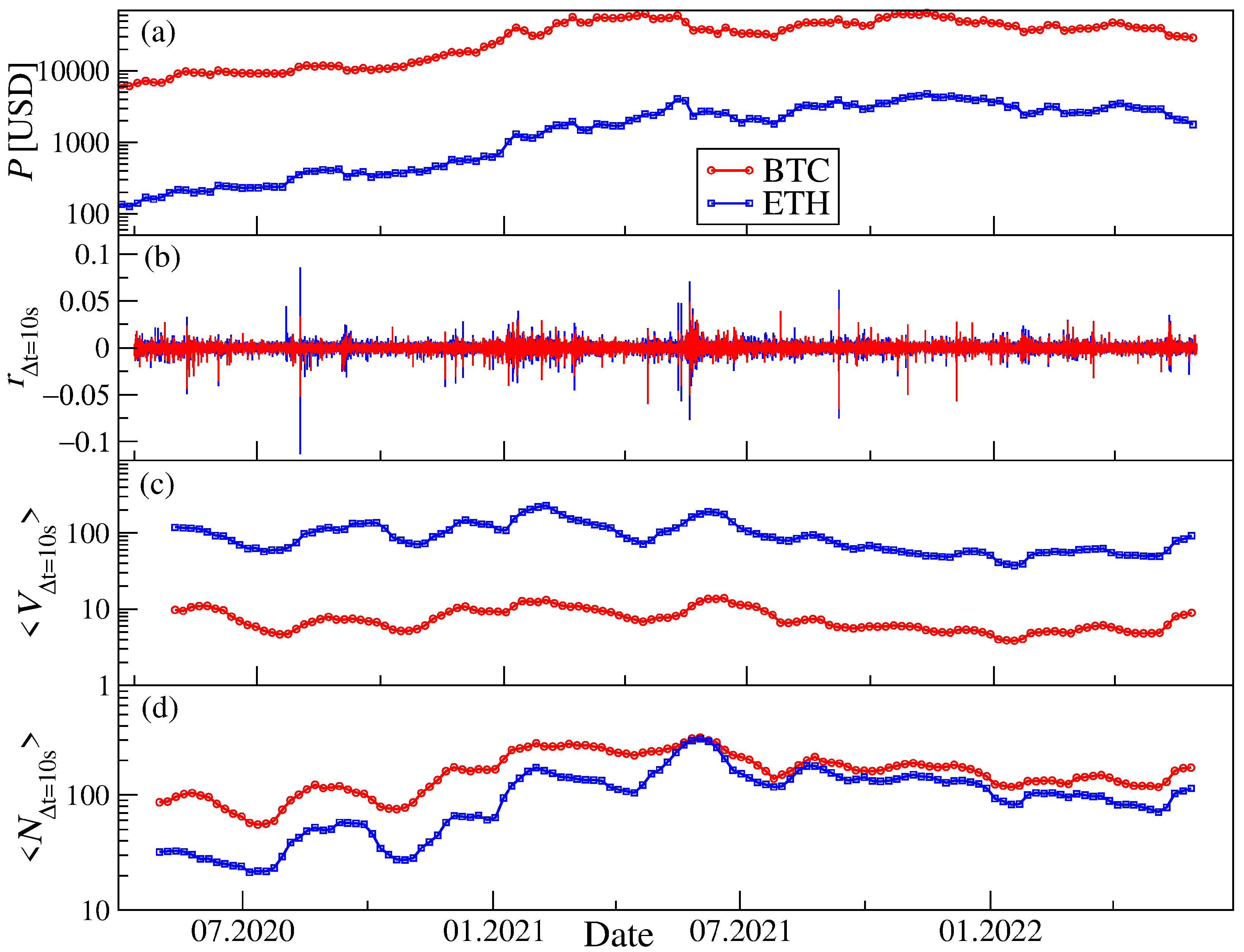
We begin the presentation by taking a look at the time evolution of the quantities of interest over the interval considered in this work. Figure 1 (top) shows the price course of BTC and ETH expressed in tether (USDT)—a stablecoin pegged (1:1 on average) to the US dollar [43]. This stablecoin is used by trading platforms as a proxy for fiat currencies, because it facilitates trading and allows the market participants to avoiding taxation while temporarily closing the cryptocurrency positions. The lowest prices of BTC and ETH during the observed 26 months were 6202 USDT and 130 USDT, respectively, recorded on 1 April 2020, and the highest prices were 68,789 USDT, recorded for BTC on 10 November 2021 and 4892 USDT for ETH, which was recorded 6 days later. The time span considered comprised almost the entire rally and subsequent fall of this market.

The logarithmic returns presented in Figure 1 (upper middle) are defined as

$$r_{\Delta t}\left(t_i\right)=lnP\left(t_{i+1}\right)-lnP\left(t_i\right),$$

(6)

where $P\left(t_i\right)$ is an asset price at time $t_i$. Inferring their heavy-tailed probability distribution function and volatility clustering is straightforward. Periods of market turbulence are associated with a high amplitude of returns. In Figure 1, a rolling window of 1 week is applied to calculate the mean volume traded $\langle V_{\Delta t}\left(t\right)\rangle$ (lower middle), and the mean number of transactions executed in 10 s-long intervals (bottom). The market sensed the most increased volatility level in September 2020, January–February 2021, and May–June 2021. These volatile periods can be associated with a few bear phases of the cryptocurrency market. The periods of increased volatility overlap with the periods of increased volume and increased number of transactions, as can be seen in Figure 1.

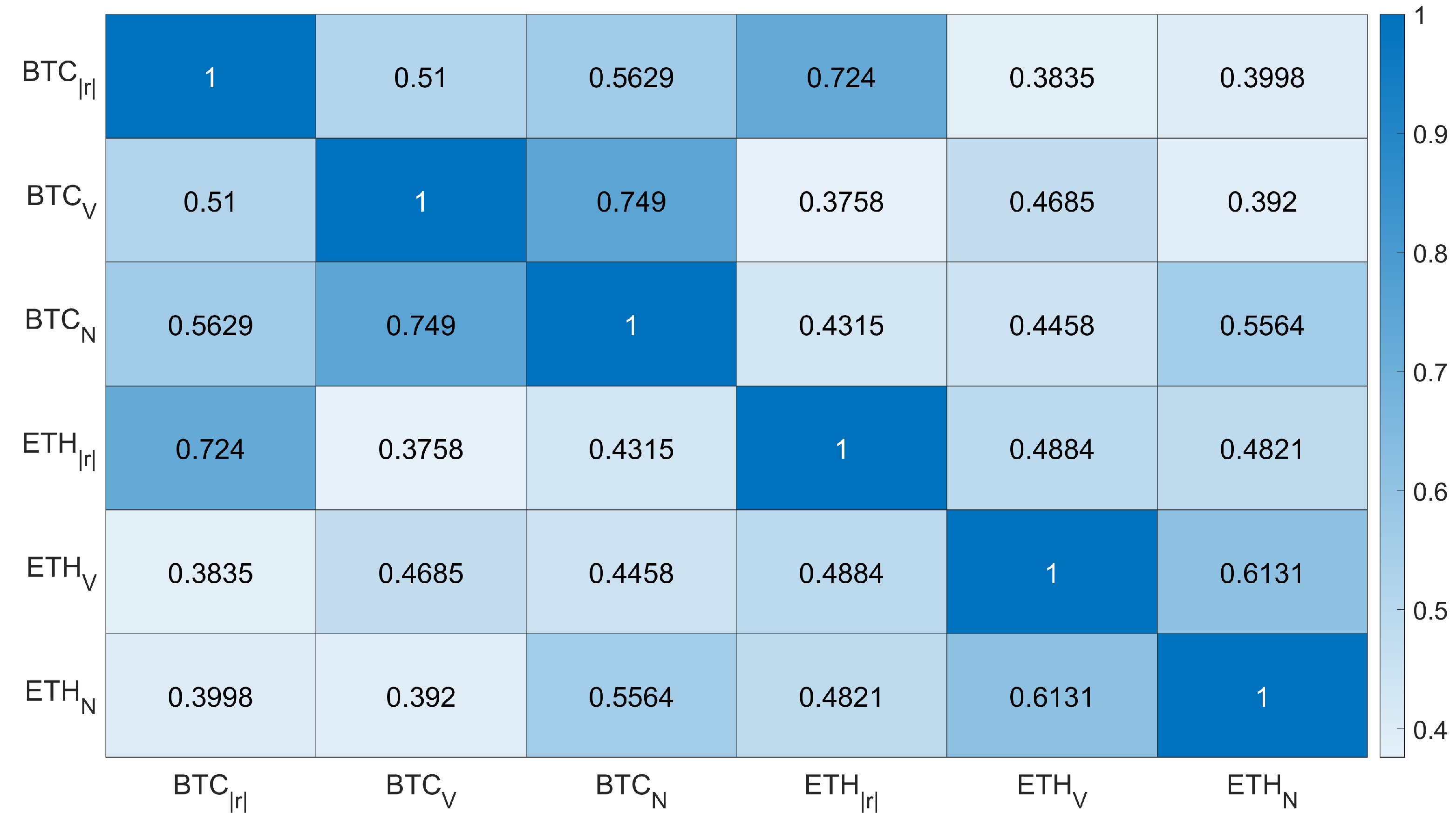
These associations can be quantified in terms of the Pearson cross-correlation coefficient

$$C_{\mathrm{XY}}=\frac{(1/T){\sum }_{i=1}^T\left(X_i-\langle X\rangle \right)\left(Y_i-\langle Y\rangle \right)}{{\sigma }_{\mathrm{X}}{\sigma }_{\mathrm{Y}}},$$

(7)

where $\langle ·\rangle$ is mean and $\sigma$ is standard deviation of the time series $\left\{X_i\right\}$ and $\left\{Y_i\right\}$. Values of $C_{\mathrm{XY}}$ for all pairs of the non-detrended time series are collected in Figure 2, showing that the strongest cross-correlations are observed for the absolute values of logarithmic returns of BTC and ETH ($C_{\mathrm{XY}}=0.72$) and for the mean number of transactions and the mean volume traded of BTC ($C_{\mathrm{XY}}=0.75$). All the related time series representing BTC are substantially cross-correlated among themselves, and the same can be noted regarding the time series representing ETH. The least cross-correlated are the pairs in which time series represent both cryptocurrencies, but even in this case, the obtained values are statistically significant.

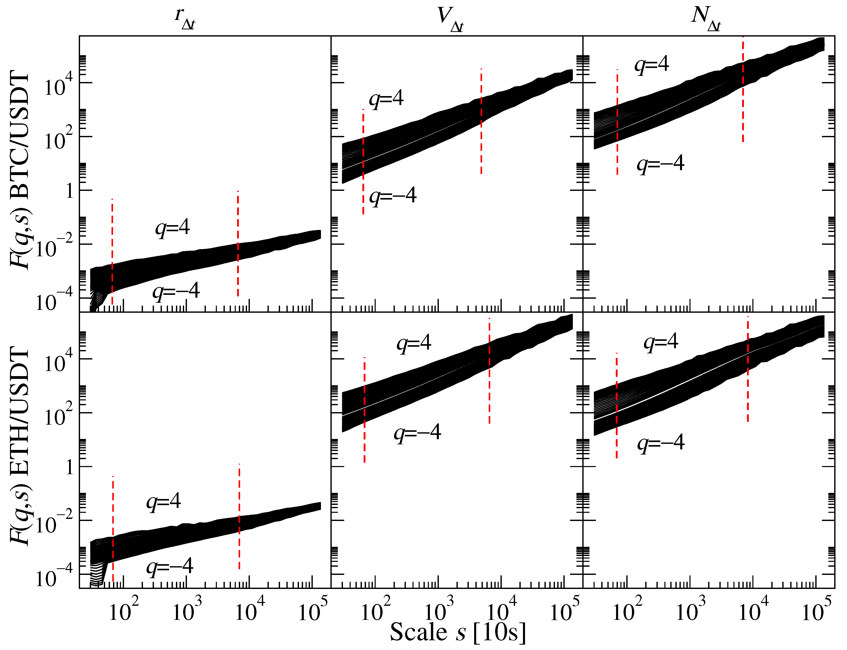
Now, we pass on to an analysis of the detrended time series. First, let us examine the fractal autocorrelations in terms of univariate fluctuation functions $F_q^{\mathrm{XX}}\left(s\right)$. The results for all time series of interest are plotted in Figure 3. All plots exhibit clear scaling for 2–3 decades for a range of q, which indicates that the time series are fractal. Moreover, a ‘broom’-like shape of the function plots for different values of q may be interpreted as a signature of the multifractal nature of time series. This result is parallel to that previously reported for the mean number of transactions executed on different trading platforms [21]. For $q=2$, we obtain the Hurst exponent H, which serves as a measure of long-term autocorrelations. One can notice that the time series for $V_{\Delta t}$ and $N_{\Delta t}$ are more persistent (a steeper ascent of $F_{q=2}^{\mathrm{XY}}\left(s\right)$) than the time series for $r_{\Delta t}$ (a milder ascent).

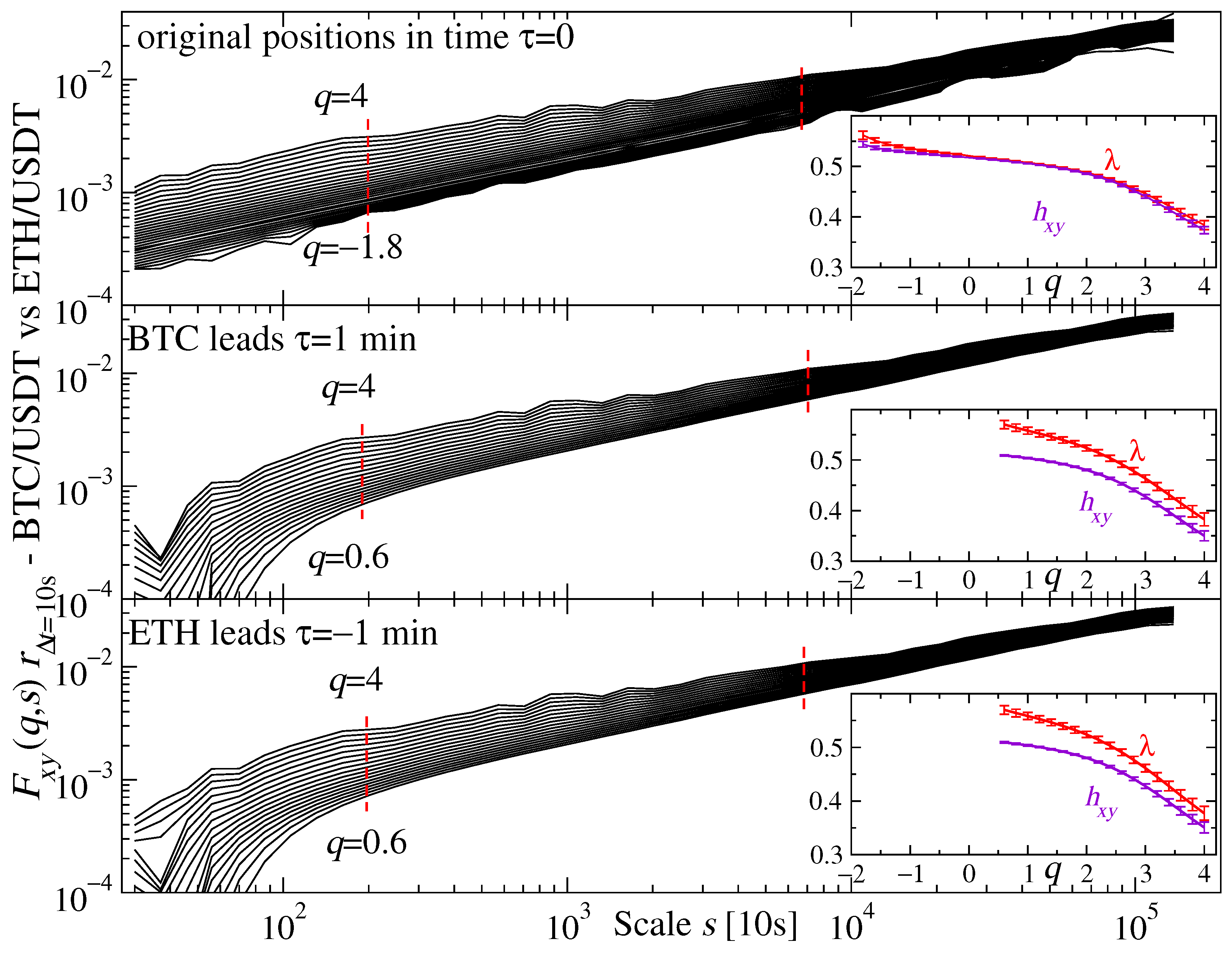
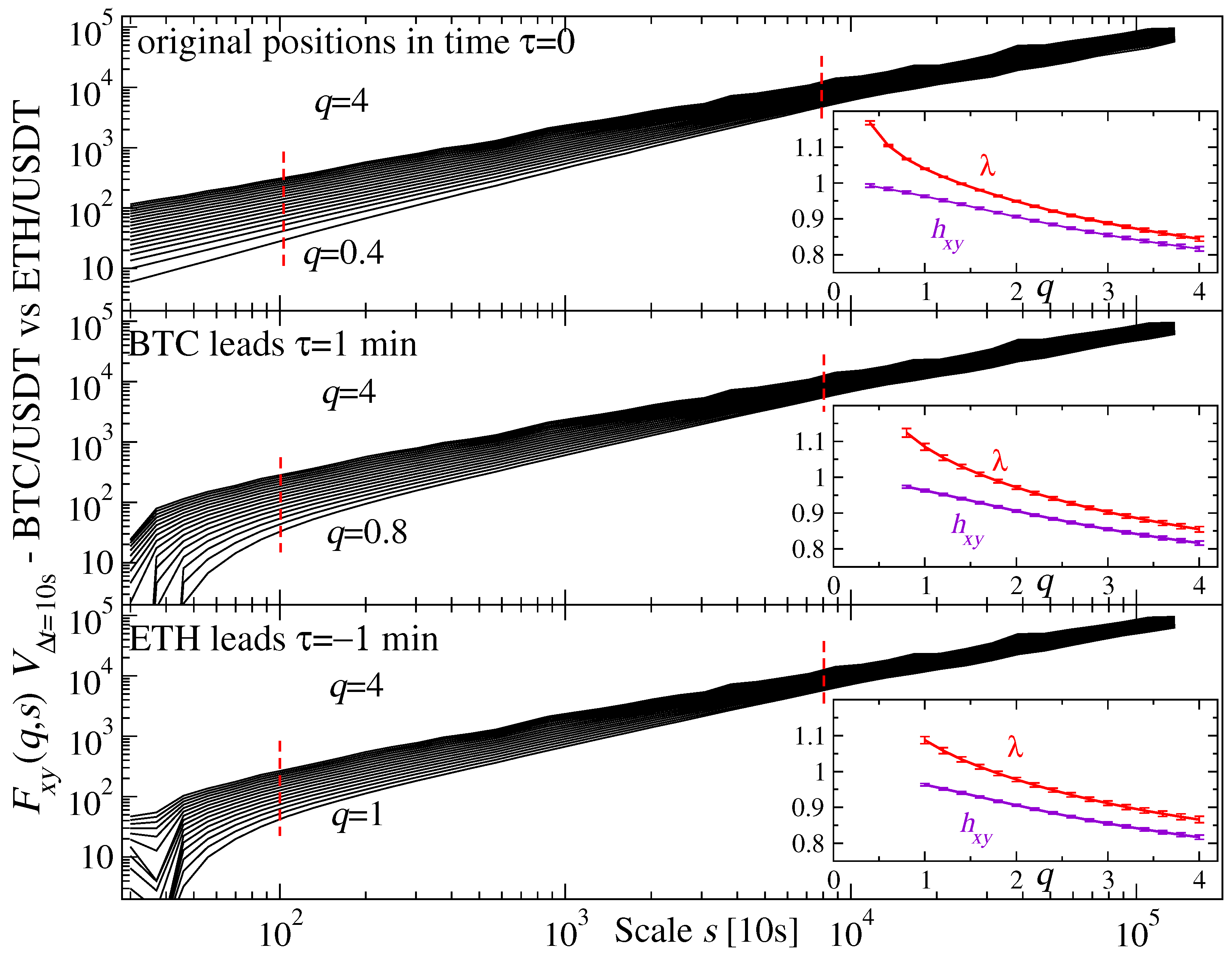
Encouraged by the values included in Figure 2 and our previous results on the price returns in the pre-COVID-19 era [44], which proved to be fractally cross-correlated, we now study the detrended cross-correlations between the time series representing BTC/USDT and ETH/USDT cross-rates. Figure 4 (top) shows the bivariate fluctuation functions obtained for three particular time series arrangements. The original time series, parallel in time, develop $F_q^{\mathrm{XY}}\left(s\right)$ that scales over ∼2.5 decades for $-1.8\le q\le 4$, which is quite extraordinary, because cross-correlations typically only scale for positive q. The insets in Figure 4 show the q-dependence of the bivariate scaling exponent $\lambda \left(q\right)$ and the mean univariate one: $h_{\mathrm{XY}}\left(q\right)=(1/2)[h_{\mathrm{X}}\left(q\right)+h_{\mathrm{Y}}\left(q\right)]$. 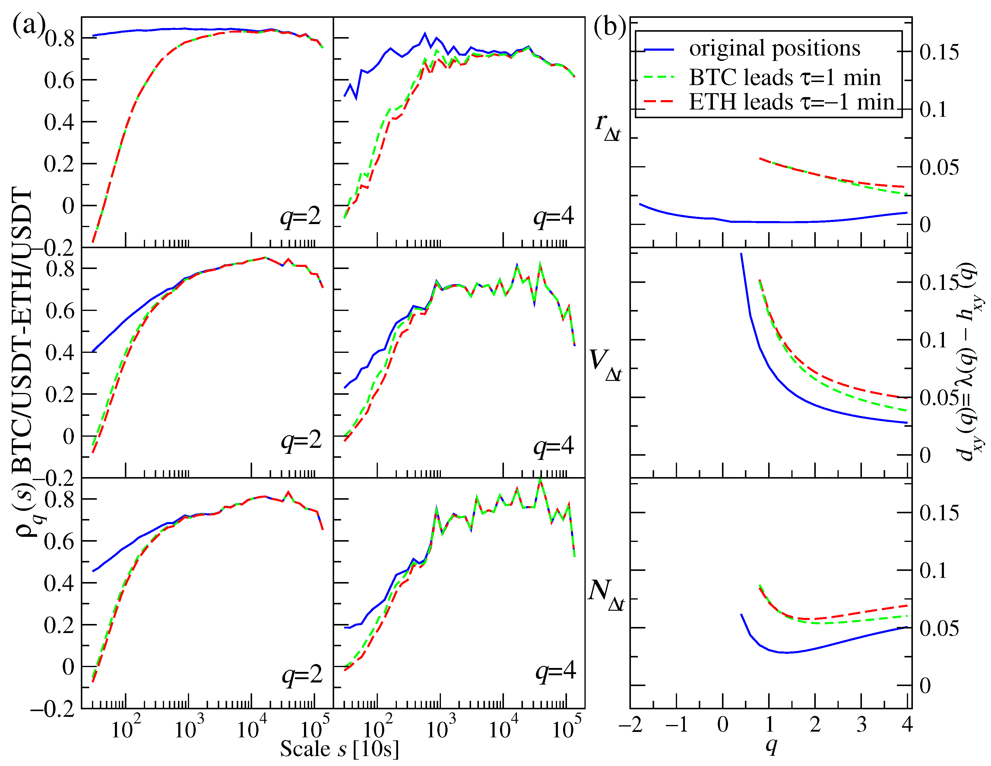Both are decreasing functions of q, which is a signature of multiscaling, and for $-2\le q\le 4$ they are equal up to their standard errors. This equality suggests that there is little difference in the scaling properties of both time series. If we look at this gap as a separate quantity $d_{\mathrm{XY}}\left(q\right)=\lambda \left(q\right)-h_{\mathrm{XY}}\left(q\right)$, we see that for $q\ge 2$ it starts to increase again slightly—Figure 5b (blue line in top panel). A relative behaviour of $\lambda \left(q\right)$ and $h_{\mathrm{XY}}\left(q\right)$ is associated with the coefficient ${\rho }_q\left(s\right)$ in such a way that if $\lambda \left(q\right)>h_{\mathrm{XY}}\left(q\right)$ for a given q, then ${\rho }_q\left(s\right)$ increases with s as the difference becomes larger. Consequently, the convergent exponents indicate that this increase in the detrended cross-correlations loses momentum with increasing q, while the divergent ones indicate the opposite [42]. Indeed, the coefficient ${\rho }_q\left(s\right)$ shows steeper growth for $q=4$ than for $q=2$ in the top panels of Figure 5a (blue lines). For $q=2$, it is even roughly constant, with only a minor decrease for the shortest scales and the longest ones.

The middle and bottom panels of Figure 4 present $F_q^{\mathrm{XY}}\left(s\right)$ for the time series that are shifted relative to each other by $\tau =1$ min: either BTC leads by $\tau$ (middle) or ETH leads by $\tau$ (bottom). In both cases, we see similar power-law dependence over ∼two decades, but for larger s than in the $\tau =0$ case. We consider this shift toward longer s as expected, because asset prices need time to build up the cross-correlations if they are weakened by the relative shifts. The bivariate and mean univariate scaling exponents shown in the insets reveal a gap between them that is largest for $q<1$, while if q increases, both quantities gradually converge. Compare this with Figure 5b (top panel, green and red lines) for even better visibility. The plots for $\tau =0$ and $\tau =\pm 1$ clearly differ from each other: for the shifted time series, ${\rho }_q\left(s\right)$ is more variable than for the simultaneous ones. However, what is similar is that here, ${\rho }_q\left(s\right)$ also shows steeper growth for $q=2$ than for $q=4$—see Figure 5a (top panels, green and red lines). For $q=2$, there is no visible difference between the results if either BTC or ETH leads (top left). This changes after we move to higher qs: for $q=4$ there is a noticeable difference between the corresponding lines, with higher values of ${\rho }_q\left(s\right)$ if BTC leads. This difference, however, is much smaller that that between the results for $\tau =0$ and $\tau =\pm 1$. This result is somehow expected, because contemporary markets operate at scales that are much shorter than 1 min. However, due to the long-range temporal autocorrelation in volatility lasting up to a few trading days [44] even if we shift one time series with respect to the other by 1 min, the fractal structure of the detrended cross-correlations can still be observed for these time series.

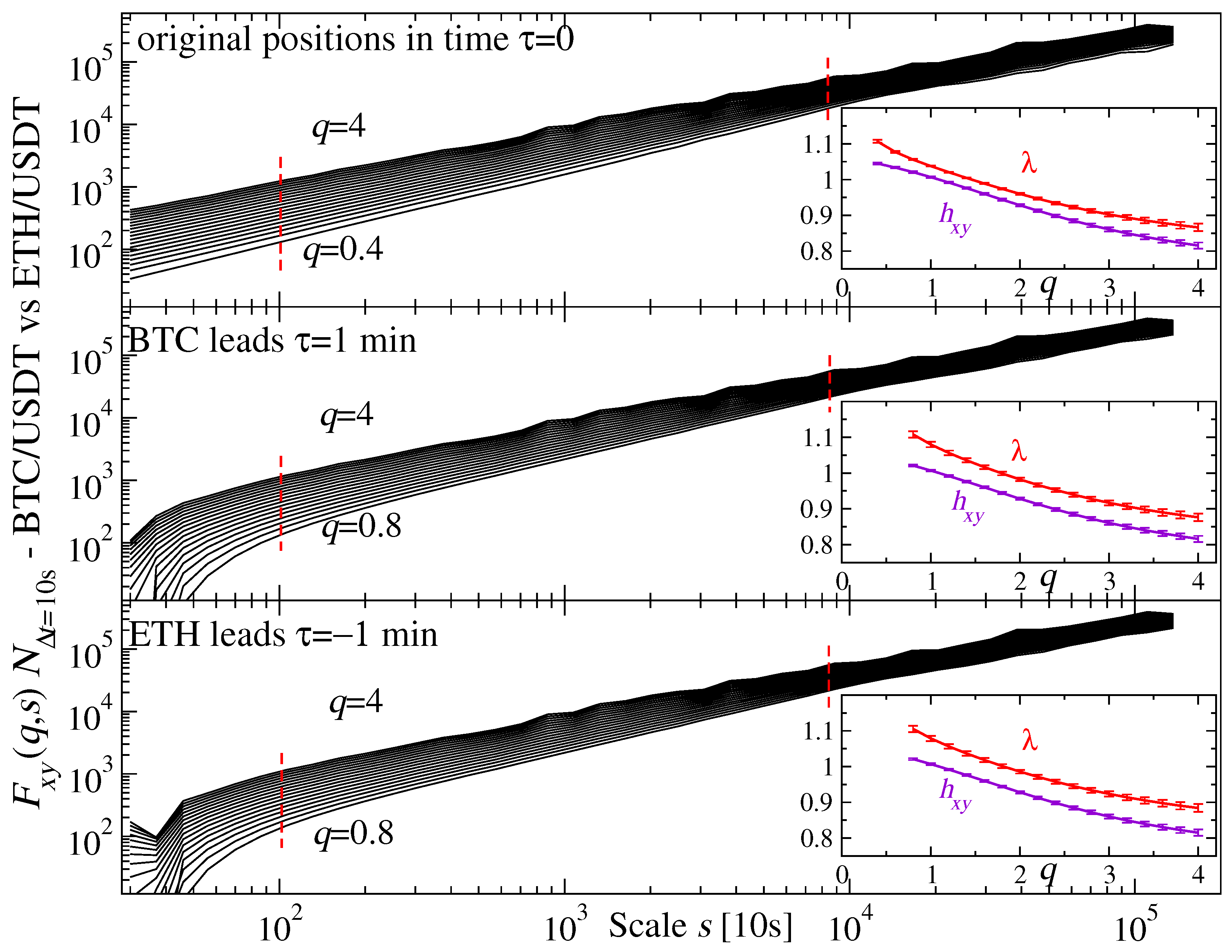
We apply the same formalism to the volume traded $V_{\Delta t}\left(t\right)$ and plot the corresponding quantities in Figure 6. There is a slightly broader range of scales for which a power-law dependence can be seen (almost two decades for the simultaneous time series and two decades for the lagged ones) than was seen for $r_{\Delta t}\left(t\right)$ in Figure 4. The range of q over which multiscaling can be detected is, however, narrower than for $r_{\Delta t}\left(t\right)$ in each case, and is restricted to positive values of q only. Another significant difference concerns $\lambda \left(q\right)$ and $h_{\mathrm{XY}}\left(q\right)$, which are sizeably separated even for $\tau =0$. For $\tau =\pm 1$ min, this difference is also more pronounced than for the price returns, but here, one can notice broken symmetry between the BTC- and ETH-led time series even in the case of $q=2$: for the advanced ETH, the difference $d_{\mathrm{XY}}\left(q\right)$ is larger than in the opposite case. This effect is also seen in Figure 5b (middle). Despite the fact that these gaps are larger, they asymptotically decrease with increasing q, suggesting that in the case of volume, ${\rho }_q\left(s\right)$ increases more slowly with s for larger q. Examples of this increase in ${\rho }_q\left(s\right)$ are plotted in Figure 5a for $q=2$ (middle left) and $q=4$ (middle right). For short scales, the detrended coefficient for the simultaneous time series ($\tau =0$) is substantially larger than for the lagged ones, while for $s>1000$ (10,000 s), this difference vanishes in both cases (for both $q=2$ and $q=4$). This effect can be understood to be such that, on sufficiently long scales, all the information that has any meaning to the market has already managed to be exchanged by the major cryptocurrencies. On the other hand, the larger values of ${\rho }_q\left(s\right)$ for $\tau =1$ min suggest that information is transferred slightly faster from BTC to ETH than in the opposite direction. This can be explained by the BTC dominance in the market. There is consistency between the respective plots for ${\rho }_q\left(s\right)$ and $d_{\mathrm{XY}}\left(q\right)$ regarding the growth ratio of the former and the magnitude of the latter for each $\tau$ and each presented q.

The behaviour of $F_q^{\mathrm{XY}}\left(s\right)$ for the time series of the mean number of transactions $N_{\Delta t}\left(t\right)$ resembles that of $V_{\Delta t}\left(t\right)$—see Figure 7 (main plots). What is different is the behaviour of the exponents $\lambda \left(q\right)$ and $h_{\mathrm{XY}}\left(q\right)$, because while we increase q, we observe that they are growing closer to each other first, then somewhere around $1.5<q<2$, they reach a minimum distance and start to diverge for larger qs (insets in Figure 7). This is even more visible in their difference in Figure 5b (bottom), which is associated with a moderate increase in ${\rho }_q\left(s\right)$ for $q=2$ (bottom left) of Figure 7a and a more pronounced increase for $q=4$ (bottom right). As in the case of volume, up to a scale of $s\approx 1000$ (i.e., 10,000 s) the coefficient is higher for the simultaneous signals than it is for the shifted ones.

4. Discussion and Conclusions

In this work, we studied the detrended cross-correlations between three trading characteristics of two major cryptocurrencies, BTC and ETH, over the last 2 years. This period was characterised by the profound stress imposed on the global economy by the COVID-19 pandemic, but after the initial shock of early 2020, when most of the markets experienced heavy losses, there was a quick rebound to new all-time highs in the second half of the year. During the pandemic, both the traditional markets and the cryptocurrency market passed through different stages, alternately governed by strong “bears” and “bulls”. Recently, the military escalation in Ukraine has also been exerting a heavy impact on the markets, including the cryptocurrency market, leading them to suffer from extra draw-downs that added momentum to the bear market dominating the scene since December 2021. From the cryptocurrency perspective, another interesting structural phenomenon is an emergent, strong permanent coupling of the cryptocurrency market and the stock market [9,44,45,46,47]—a phenomenon that, prior to the pandemic, used to be observed only occasionally [8,48,49,50,51,52,53].

Financial market data are well-known for their nonstationarity. This is why the classical approach to quantifying correlations among such data in terms of, for instance, the Pearson coefficient can overlook important properties of the data. The formalism based on the detrended fluctuation analysis [54] and its further generalisations [37,38,39,40] are much more suited for non-stationary signals, as their inherent feature is the elimination of multiscale trends. At present, this approach is favoured and becomes a standard tool of time series analysis. In our work, this formalism was employed to investigate cross-correlations between two major cryptocurrencies—BTC and ETH. We selected three trading characteristics: price returns, volume, and number of transactions in a time unit (for which we chose 10 s). We did not restrict the analysis to the time series collated parallel in time, but we also analysed the ones that were shifted relative to each other by 1 min. By looking at the univariate and bivariate fluctuation functions, we found that both were manifesting the multifractal property. Only the results for the price returns can be directly compared with the analogous results obtained for the data covering earlier periods before COVID-19 [44,55,56,57,58,59]. In this case, we see that the fractal properties of the price returns have not changed much. This is true not only if we look at the fluctuation functions, but also at the bivariate and mean univariate scaling exponents, which are almost equal in this case.

We also analysed the lagged cross-correlations between the time series representing BTC and ETH for the first time in the literature. We found that shifting one of the time series suppresses the cross-correlation magnitude, but nevertheless, the remaining cross-correlations are still significant, especially for the scales larger than a few hours, during which the information that arrives on the market is able to disperse. The time series of the price returns did not reveal any asymmetry between the cases, in which either BTC or ETH is lagged, for $q=2$. However, the time series of the volume traded and the number of transactions showed a small effect of such an asymmetry: if BTC led, the cross-correlation was slightly stronger, which we interpreted as an effect of faster information transfer in the direction BTC→ETH than in the opposite direction, which we related to the BTC dominance on the cryptocurrency market. Interestingly, for $q=4$, this asymmetry is easy to notice in the case of the returns as well—a manifestation of a fact that the correlations associated with the returns of large amplitude are more direction sensitive than the correlations associated with the small and medium returns. Another observation was that, for short scales, the strength of the cross-correlations between the simultaneous time series representing BTC and ETH was the largest for the price returns, whereas for the volume and the number of transactions, it was substantially smaller. This effect was less pronounced for the lagged time series, and it gradually disappeared for the longer scales.

A general conclusion that we can draw from this study is that the overall fractal properties of the major cryptocurrency time series are stable regarding the pre-COVID-19, COVID-19, and post-COVID-19 periods. We can interpret this stability as related to the fact that the processes that govern the fractal organisation of the cryptocurrency trading data are so fundamental that they can resist the social and economical forces perturbing the market. This conclusion apparently challenges some earlier reports based on stock market data, whose fractal properties were market-phase dependent (e.g., [60]), but actually it must be noticed that here, we did not attempt to decompose the market dynamics, and we presented the average market properties only. As the fractality indicates that the processes driving the cross-asset trading characteristics are largely scale invariant, our result can be of significance from the market-modelling perspective. It also provides further support for the thesis that the cryptocurrency market has reached maturity, at least from the statistical and dynamical points of view.

It should be noted, however, that our study has its inherent limitations. We analysed two major cryptocurrencies only; it is thus conceivable that results for other cryptoassets, especially those with much worse liquidity, would potentially diverge from the results presented here. We also stress that we restricted our analysis to a few values of time lag. If another study considered different lags, especially the shorter ones, both the the cross-correlation magnitude and the asymmetry effect could be different. We also analysed a particular time period only, while the history of the cryptocurrency market is much longer. We could thus expect that the properties of the lagged cross-correlations evolve in time as well. Each of these limitations should be overcome in future research based on extended data. Another issue to be considered in future is to focus on short periods of time in order to gain some insight into how the fractal cross-correlation magnitude and lag asymmetry depend on the market situation (the bull and bear markets, for instance).