Energy-Optimized Content Refreshing of Age-of-Information-Aware Edge Caches in IoT Systems

Abstract

The Internet of Things (IoT) brings internet connectivity to everyday devices. These devices generate a large volume of information that needs to be transmitted to the nodes running the IoT applications, where they are processed and used to make some output decisions. On the one hand, the quality of these decisions is typically affected by the freshness of the received information, thus requesting frequent updates from the IoT devices. On the other hand, the severe energy, memory, processing, and communication constraints of IoT devices and networks pose limitations in the frequency of sensing and reporting. So, it is crucial to minimize the energy consumed by the device for sensing the environment and for transmitting the update messages, while taking into account the requirements for information freshness. Edge-caching can be effective in reducing the sensing and the transmission frequency; however, it requires a proper refreshing scheme to avoid staleness of information, as IoT applications need timeliness of status updates. Recently, the Age of Information (AoI) metric has been introduced: it is the time elapsed since the generation of the last received update, hence it can describe the timeliness of the IoT application’s knowledge of the process sampled by the IoT device. In this work, we propose a model-driven and AoI-aware optimization scheme for information caching at the network edge. To configure the cache parameters, we formulate an optimization problem that minimizes the energy consumption, considering both the sampling frequency and the average frequency of the requests sent to the device for refreshing the cache, while satisfying an AoI requirement expressed by the IoT application. We apply our caching scheme in an emulated IoT network, and we show that it minimizes the energy cost while satisfying the AoI requirement. We also compare the case in which the proposed caching scheme is implemented at the network edge against the case in which there is not a cache at the network edge. We show that the optimized cache can significantly lower the energy cost of devices that have a high transmission cost because it can reduce the number of transmissions. Moreover, the cache makes the system less sensitive to higher application-request rates, as the number of messages forwarded to the devices depends on the cache parameters.

1. Introduction

The Internet of Things (IoT) brings internet connectivity to everyday objects and devices, such as wearables, sensors, actuators, etc. These IoT devices generate a large amount of data that is then transmitted to IoT applications, where they are analyzed to make some output decisions. These output decisions are directly related to the freshness of the received data. Indeed, delivering fresh status information of the underlying process is critical for many IoT applications for effective monitoring and control, and the number of these IoT scenarios in which devices send time-stamped status updates to applications is continuously growing. For example, sensor data are analyzed to detect anomalies; environmental sensor data can help to predict and control fires or other calamities; or, as another example, vehicles share their positions, velocities, accelerations, etc. to assist drivers in an intelligent transportation system. This phenomenon is even more evident in the Industrial IoT (IIoT) context. IIoT applications require continuous updates about the real-time states of a huge volume of devices, e.g., a smart manufacturing application requires receiving fresh telemetry data from the sensors of the assembly line, possibly to determine if an actuation request is needed. Ideally, we would want a device to generate status updates as fast as possible and transmit them to the application; however, the deployment of such systems raises several challenges as the timeliness of this huge amount of status updates is limited by the severe energy, memory, processing, and communication constraints of IIoT devices and networks. In particular, energy is a scarce and crucial resource, as devices may not have a fixed power supply, but they may rely on batteries, or they may harvest energy. So, the generation and the transmission of the device status updates need to be managed effectively to save energy on the device and prolong its lifetime: this is fundamental in massive deployments where human intervention is limited. The energy consumption of the device depends mainly on two factors: the sensing energy consumption, i.e., the energy used to obtain the newest status information, and the transmission energy consumption, i.e., the energy used to transmit the status information [1]. Modern IoT devices can perform complex operations other than the typical simple monitoring tasks. For example, they can use on-device artificial intelligence to pre-process the sensed information, so generating a status update can be very expensive in terms of energy. Moreover, a packet generated by one of these complex tasks, e.g., an artificial intelligence task, can convey more information than a packet generated by a simple monitoring task, so the energy cost for transmitting it can be higher [2]. Finally, even for simple monitoring tasks, the sensing energy cost may vary greatly: for passive sensors, such as temperature sensors, sensing power consumption is negligible in comparison to other devices, while for active sensors, such as gas sensors, sensing power consumption can be significant [3]. The transmission energy cost may also vary depending on the underlying transmission technology: some transmission protocols are more energy-efficient due to LPWAN technologies [4].

Within this context, the objective of IoT-system management is to minimize the energy consumed by the device for sampling the physical process of interest and for transmitting the data, while ensuring the requested level of information freshness is provided. One possible solution is using an information caching system: indeed, caching the data generated by the device can be very effective in reducing the sensing frequency and the transmission frequency. However, caching can lead to the staleness of information, so the cache needs a refreshing scheme, as IoT applications need timeliness of status updates.

Sending update messages as soon as they are available may not guarantee the timeliness of status updates: the IoT application may receive delayed updates as the messages may congest the network; on the other hand, also reducing the number of transmitted messages may not guarantee the timeliness of status updates—the IoT application may receive outdated messages because of a lack of updates. So, several measures have been analyzed in order to measure the freshness of the cached data [5] and consequently to design a refreshing scheme for the cache. One of the most used is the Age of Information (AoI) metric since it is a suitable metric for describing the freshness at the receiver with respect to the sender. Introduced in [6], the AoI is defined as the elapsed time for an item between the current time and the time the item was generated at the source, i.e., the IoT device [7,8]. Typically, applications establish a threshold on the value of the AoI; hence, it may be necessary to optimize the system so that the AoI remains below this threshold with a certain probability [9]. This means that at least a fraction of the application requests should receive a data item whose AoI is not larger than the threshold.

In a preliminary version of this work [10], we proposed an AoI-aware model-driven cache-management scheme implemented in an edge-based proxy. The proxy can efficiently use a network, computing, and storage resources at the edge, and it can leverage the proximity with the IoT devices to optimize their communication with the IoT applications [11]. Since IoT data typically have a lifetime during which they are useful, we considered a cache-refreshing scheme that associates a lifetime, called refresh window, and expressed in terms of AoI, to each cached item. So, the IoT application requests are sent to the proxy that responds using the cached item if its AoI is smaller than its refresh window; otherwise, it fetches the latest sample from the IoT device, delivers it to the application, and refreshes the cache. This results in a simple polling scheme that can be deployed even on a resource-constrained proxy. We proposed a model for this cache-management scheme that allowed us to derive the closed forms of the average time between two requests that cause a refresh of the cache, i.e., the average time between two polls, the average AoI of the data at the application, and the probability distribution function of AoI.

In this work, we leverage our model described in [10] to configure the sampling period of the device and the refresh window of the cache. Our main contributions can be summarized as follows:

• We define a model-driven optimization problem to set the sampling frequency of the IoT device, and the value of the refresh window of the cache so that the device power consumption is minimized, while the AoI requirement expressed by the IoT application is satisfied. The device power consumption depends on the energy consumed to transmit the messages and the energy consumed to sense the environment.
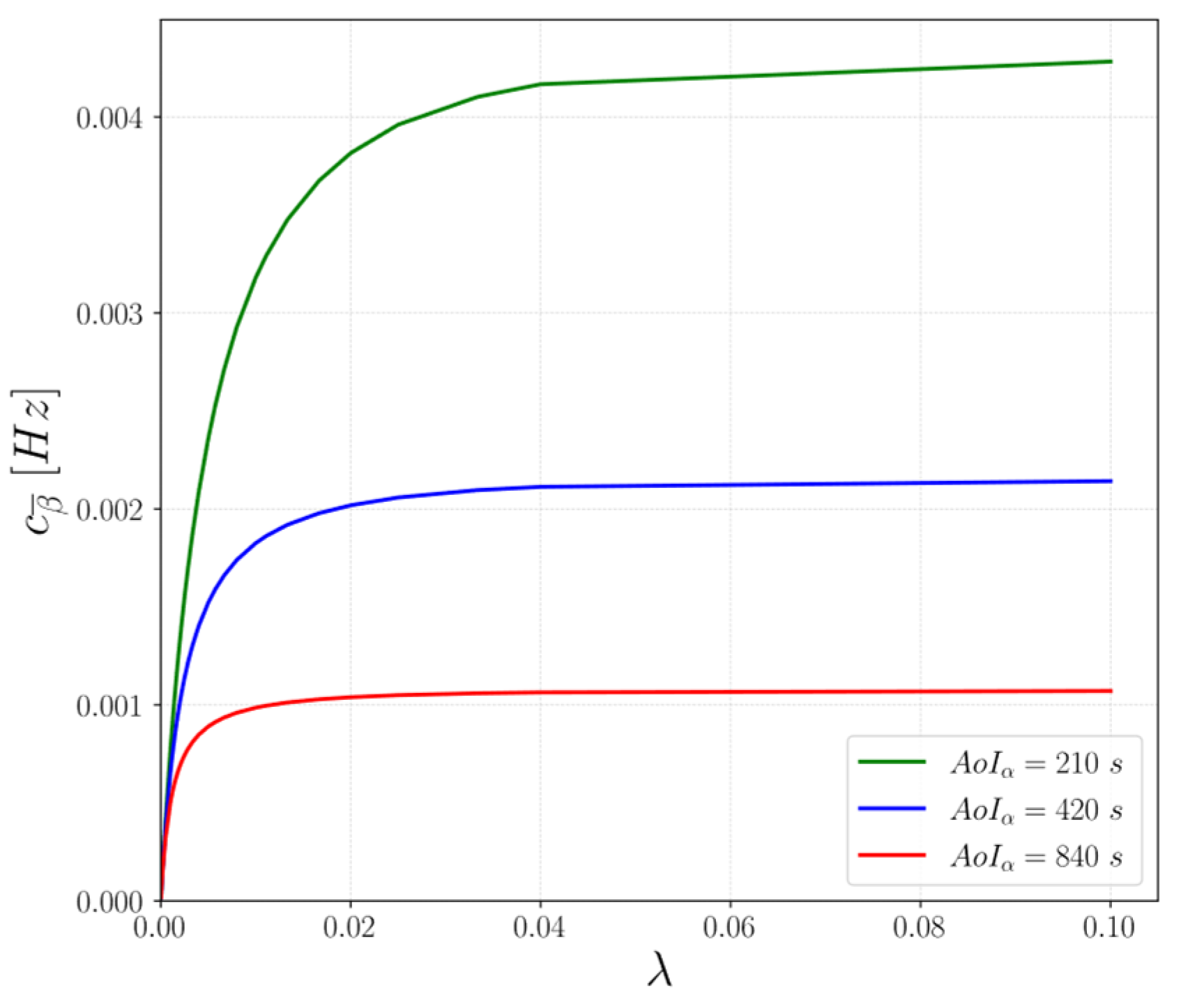
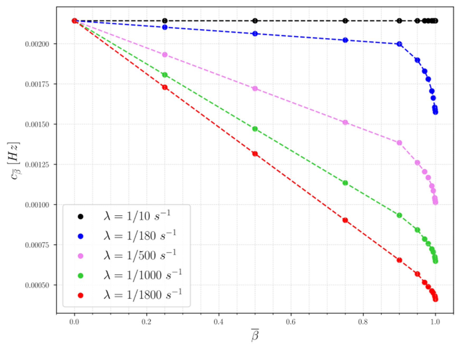
• We solve the optimization problem, and we provide an extensive numerical evaluation of our cache-management scheme, showing the trade-off between minimizing the energy consumed to transmit the messages and the energy consumed to sense the environment.
• We evaluate the performance of our cache-management scheme in a realistic environment based on an emulated IoT network using the OMA LightweightM2M ([12,13]) protocol for IoT device management. In the experiments, we consider a sample scenario composed of an LWM2M Server, i.e., the IoT application, an LWM2M Client, i.e., the IoT device, and an LWM2M Proxy located in between them. The LWM2M Proxy implements the proposed cache management scheme to improve system performance [11], and the refresh window of the cache is selected using the proposed optimized method. We show that the proposed method chooses a refresh window that minimizes the energy cost while satisfying the AoI requirement.

The remainder of the paper is structured as follows: Section 2 discusses the related work, whereas Section 3 describes the proposed model. Section 4 describes the proposed method to configure the cache parameter, Section 5 illustrates performance evaluation. Conclusions are drawn in the last section.

2. Related Work

Energy-efficient IoT solutions and IoT-network life span are the key challenges for enhanced smart cities, smart grids, smart transport systems, etc. [14]. So, energy management is a critical issue in designing IoT networks, since many IoT devices can rely only on limited battery power and it is often unfeasible to replace or recharge their batteries. Therefore, efficient energy management strategies should be implemented in IoT devices to prolong their lifetime; for example, in [15] Naeem et al. propose an energy-efficient routing protocol to enhance network lifespan, or in [16] Dev et al. optimize energy utilization through an optimal cluster head selection. In general, IoT devices consume energy, especially in sensing the environment and processing the acquired data, and transmitting their updates. However, the energy management strategies must guarantee the freshness of data, which is typically quantified using the AoI metrics. For example, in [17] Abbas et al. devise a discrete-time Markov chain model to predict the values of AoI and the probability of packet drops in status update systems, investigating the effects of the arrival rates of the packets, the number of nodes, and the queue length of each node. In [18] Akar et al. propose a discrete-time queueing model to derive the distributions of AoI and Peak AoI in multisource IoT-based status update systems under the assumption of Bernoulli information packet arrivals and a general discrete phase-type service time distribution across all the sources. So, several works studied the problem of designing an optimum sampling and updating policy for the device. For example, in [2], Zhou et al. designed an optimal status sampling and updating policy for an IoT device to minimize the AoI of the data at the destination, under an average energy cost constraint at the device. As another example, in [19] Kaul et al. face the problem of keeping the status updates of the sources as timely as possible to all their monitors; they consider the first-come-first-served queue policy and show the existence of an optimal rate at which a source should generate its updates. In [20], Abd-Elmagid et al. investigated an optimal sampling policy that minimizes a long-term weighted sum-AoI. In [21], Chiarotti et al. proposed the Age of Information at Query (QAoI) measure to characterize the AoI available to the receiver when it needs it; they considered a sensor that needs to schedule transmissions over a link with limited availability and they maximize the freshness of the data at query time, considering that the sensor needs to limit the number of transmissions to prolong its lifetime.

Since IoT devices use near-range technologies, they cannot communicate directly with applications usually deployed in the cloud: for this reason, IoT networks are typically accessed through gateways/proxies acting as intermediaries between IoT devices and IoT applications. So, these intermediary nodes can be leveraged to also provide better performance in terms of energy consumption. For this purpose, caching the data generated by the devices can be very effective because it can lower the power consumption, reducing the frequency of environmental sensing and the frequency of data transmissions. So, for example, in [22] Niyato et al. introduced the use of a cache for an IoT sensing service with energy harvesting. Indeed, since the IoT sensor has a limited and random energy supply, caching can help to reduce the number of requests sent to the sensor and, therefore, can lower its energy consumption. The cache is deployed at a gateway and its refreshing scheme is a timer threshold mechanism: a cached item has a timer and, if the timer is larger than the threshold, the cache assumes that the item is expired, activates the sensor, and obtains a fresh sensing result. In [23], Xu et al. quantify the data freshness using the AoI metrics and formulate an update optimization problem for the cache to minimize a cost that considers the users’ AoI and the sensor’s energy consumption. Instead, other works design cache refreshing schemes to balance AoI and latency. For example, in [24], Zhang et al. proposed two cache-refreshing schemes: in the first one, the cached items are updated in a round-robin manner; in the second one, the cached items are updated upon requests with a certain probability. However, both the proposed schemes may lead to unnecessary cache refreshing because they do not take into account the current state of the cached data. In [25], Zhang et al. proposed a cache-assisted lazy update and delivery (CALUD) scheme to balance content freshness and service latency in vehicular networks. In [26], Zhang et al. proposed a cache-refreshing scheme where the cached items are refreshed upon user requests if their AoI exceeds a given threshold called refreshing window; then, the value of the refreshing window is set solving an optimization problem that minimizes the average delay under the average AoI constraint of all sources. However, a requirement about the average AoI does not give any guarantee about how AoI values are distributed, so it is not possible to express a requirement in terms of the percentile of the distribution. Moreover, it is not possible to take into account the energy consumption due to the sampling operations, as they consider a device that generates updates on demand, i.e., the AoI at the device is always zero. It is thus not possible to apply this solution for devices having a periodic sampling behaviour. In this work, we propose a model-driven cache-management scheme to configure the parameters of a cache deployed on an edge-based IoT proxy. More in detail, we define and solve an optimization problem that aims at minimizing the energy consumption on the device and consider the freshness of the data, expressed in terms of AoI, as a constraint. The cache system could also be managed using data-driven schemes [27]; however, we aim to propose a simple cache-management scheme so that it can easily scale in case of massive IoT deployments.

3. System Overview and Model

A typical IoT system consists of the following three main components [28] (see Figure 1a):

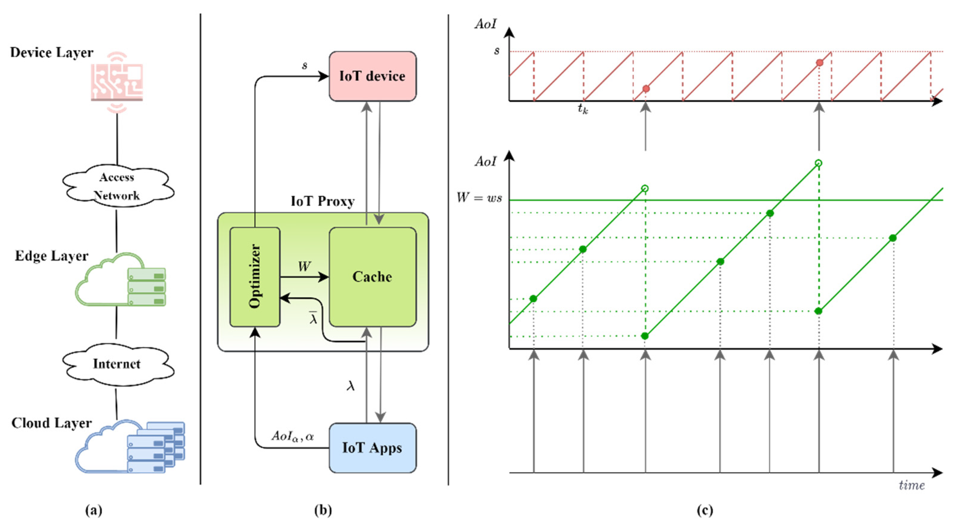
• IoT Devices: they collect data or perform actuation, e.g., they are either sensors or actuators, and they have communication capabilities to submit the data to the broader IoT system through an access network.
• IoT Applications: they typically run in the cloud and play three main roles: (i) data acquisition, storage, and access, to support the generation of a huge amount of data from devices, which is then stored to be processed and analyzed; (ii) data analytics on the collected data, which are examined to detect valuable information to support, for example, decision making; (iii) actuation support. In addition, they support several administrative functions, such as device management, user-account management, etc.
• IoT Gateways/Proxies: they collect, process, and transfer data from devices to applications and deliver the actuation requests from applications to devices. They may also act as intermediaries between the devices and the applications, e.g., they may support data storage, service discovery, etc.

3.1. System-Model Overview

Without loss of generality, in the following, we consider a scenario composed of a single IoT device, a Proxy, and a single IoT application running on a server deployed in the cloud, as sketched in Figure 1b. The proposed system model can be applied for each application and for each device managed by the proxy.

3.1.1. IoT Device

In many scenarios, devices collect information at a specific sampling rate, and, among the sampling behaviors, periodic sampling is the most prevailing behavior used by real-world applications [29]. Indeed, the simplicity of periodic sampling is well-fitted with constrained devices, which have limited computational resources; for this reason, it is widely used for IoT devices [4]. So, we assume that the IoT device performs measurements periodically with a sampling period $s$, which can be configured. We assume that the sampling period cannot be smaller than a given value called $s_{min}$, which is due to physical limitations on the device hardware. We denote $t_k$ as the time when the $k$-th sample is collected. The fact that the device collects information at a given sampling rate implies that any external query on the device itself will produce data having an AoI in the range between 0 and $s$.

3.1.2. IoT Application

A server typically deployed in the cloud runs the IoT application that needs to retrieve the state of the IoT device as a part of, for example, a monitoring or control process. The server generates requests for state updates of the IoT device and forwards them to the proxy. We assume that the generation of requests is a process with a mean rate $\lambda$. As we mentioned in the Introduction, applications can require that the AoI of the received data remains below a threshold with a certain probability. Hence, the application-freshness requirements are formulated as follows: the IoT application requires that at least a fraction $\alpha$ of the requests receive a data item whose AoI is not larger than a target value denoted by $Ao{I}_{\alpha }$ (see Figure 1b). As an example, an IoT application requires that at least 90% of the requests, i.e., $\alpha =0.9$, receive a data item whose AoI is not larger than a given target value, i.e., $Ao{I}_{\alpha }$.

3.1.3. IoT Proxy

We propose to deploy the IoT proxy at the network edge, in between the IoT devices and the IoT application. Hence, it can efficiently use a network, computing, and storage resources at the edge to overcome the limits imposed by IoT devices and networks [11]. More in detail, we propose that the proxy implements a cache: it tries to respond to server requests using the cached items, thus reducing the energy consumption on the device. However, caching may lead to the staleness of information, while the IoT application demands timeliness of status updates, so the cache needs a refreshing scheme. Typically, a cache associates a validity lifetime to each stored item and when the lifetime expires, the item is not fresh anymore and should be discarded. Several measures have been introduced to quantify the freshness of a cached item [5] and, among them, AoI is one of the most used [7]. We choose then to evaluate the freshness of a sample using the AoI metrics: in our cache refreshing scheme, a cached item is considered fresh if its AoI is smaller than a refresh window, called $W$. The proxy responds to the server request using its cached item if it is valid; otherwise, it updates the cache fetching the latest sample from the IoT device and then delivers it to the server. Since this caching mechanism has constant complexity, as it involves only a comparison between the AoI of the cached item and its refresh window, it can easily scale if the proxy has to manage multiple devices. Figure 1c shows an example of the relationship over time between the arrival process of requests from the IoT application, the periodic sampling on the IoT device, and the cache operation on the proxy. Moreover, we assume that before starting to exchange messages, there is a setup phase during which the IoT application specifies its freshness requirements to the proxy in terms of a target percentile $Ao{I}_{\alpha }$ for a given threshold $\alpha$.

The cache system implemented by the proxy Is then composed of a cache with parameter $W$ and an optimizer that sets the most suitable value of $W$ (see Figure 1b). $W$ is the solution to an optimization problem that minimizes the cost in terms of energy consumption at the IoT device while satisfying the AoI requirements of the IoT application. The energy cost depends on the energy consumed to transmit the update messages and the energy consumed to sense the environment. The optimizer takes as inputs the AoI requirements, i.e., $Ao{I}_{\alpha }$ and $\alpha$, and the (estimated) average request rate $\lambda$.

We assume that the network between the proxy and the server that runs the IoT application, and the access link between the proxy and the IoT device are both ideal, i.e., there is no transmission error. Moreover, being deployed at the edge [11], the proxy can take advantage of the proximity to IoT devices; hence, it experiences small and predictable network delays as compared to AoI requirements. For this reason, it should not be deployed farther from the device. However, the proxy should not be deployed closer, e.g., in a device of the access network itself. Indeed, in the case of a dynamic IoT scenario, e.g., a scenario involving topology changes, a proxy deployed in a device of the access network might fall in a sub-optimal placement with respect to the device-application path. Instead, node mobility is transparent to an edge-based proxy, as it is typically supported by the routing protocol or the handover function of the access network itself. We also assume that the link between the proxy and the server is almost deterministic, so the application can simply take the link delay into account when expressing the freshness requirement. Therefore, they are both assumed to be null in the following derivations.

3.2. Model of the Cache-Management Scheme

Here, for the sake of completeness, we briefly report the model of the cache management scheme we proposed in [10], which is the basis for the optimization method proposed in this work.

We model the cache-management scheme as a $2w$-states Discrete-Time Markov Chain (DTMC) ${\left\{X_k\right\}}_{kϵ\mathbb{N}}$, where transitions occur at time instants $t_k$. We assume that the generation of server requests follows a Poisson distribution with an aggregate rate $\lambda$. We also assume that the cache parameter $W$ is a multiple of the device sampling period, i.e., $W=ws$ with $w\ge 1$. The discrete-time Markov chain is a simple yet effective model that allows us to derive in closed forms the following system KPIs: the average AoI of the items and their distribution at the steady-state, and the number of transmissions per unit of time needed to update the cache. This model makes only a few assumptions on the underlying system, i.e., we only assume that the edge-based proxy experiences small delays as compared to AoI requirements, and that the link between the proxy and the server is almost deterministic. Finally, the probability distribution function of the AoI can be used for the model-driven optimization of the cache.

States: We denote $X_k$ as the state of the DTMC at time $t_k$. $X_k$ is defined by two components: (i) the first specifies if in the previous interval $\left(t_{k-1},t_k\right)$ at least one request has arrived; (ii) the second specifies the number of remaining intervals during which the cached item is still considered fresh. Hence, the states of the DTMC are the following (see Figure 2):

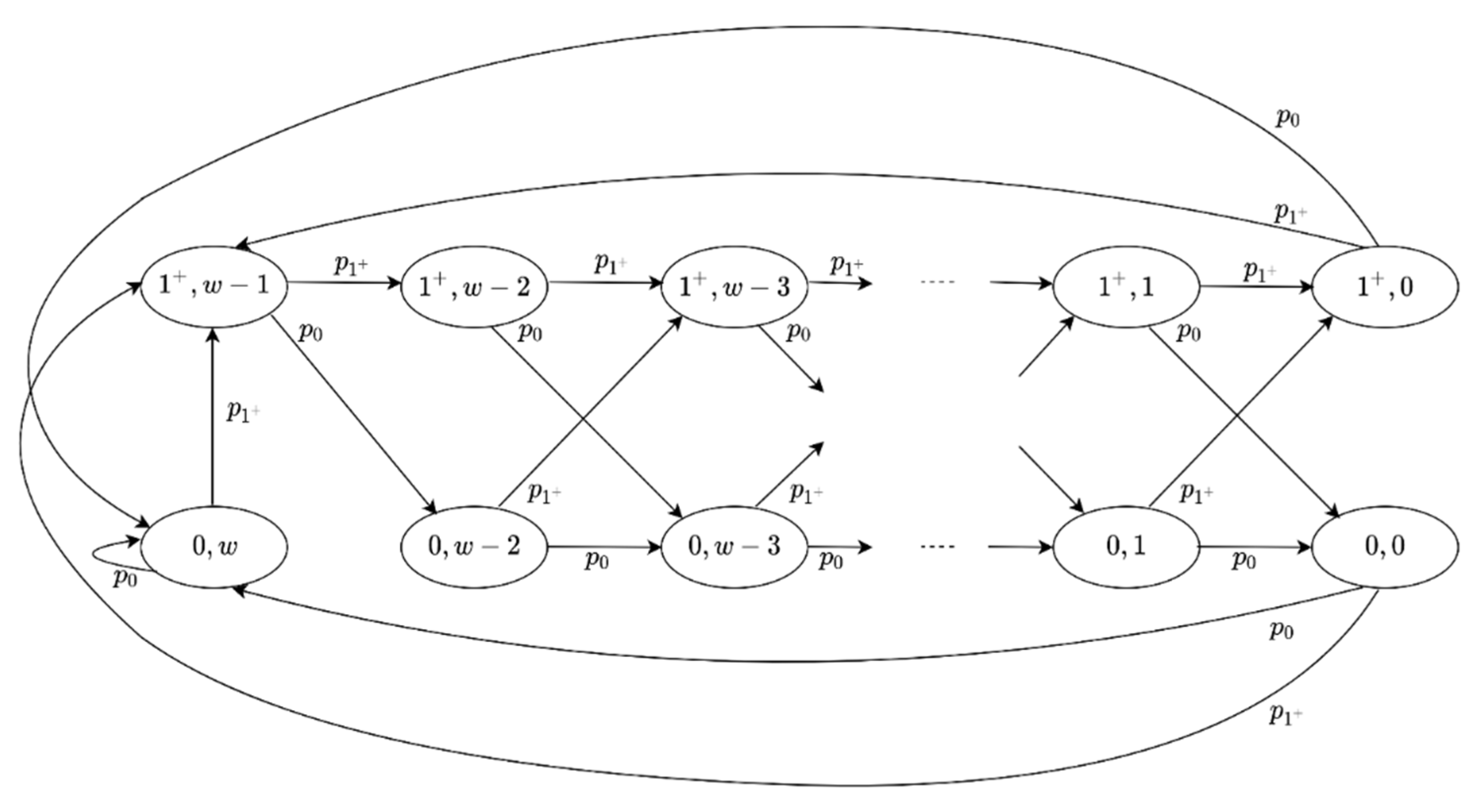
• $X_k=\left(0,w\right)$: no request arrived during the interval $\left(t_{k-1},t_k\right)$ and there is not a fresh item in the cache. So, if a request arrives in the interval $\left(t_k,t_{k+1}\right)$, the proxy fetches the latest update from the device, which will be cached and will expire in $w$ intervals.
• $X_k=\left(0,w-j\right)$, $1<j\le w$: no request arrived in the interval $\left(t_{k-1},t_k\right)$, and the cached item will expire in $w-j$ intervals.
• $X_k=\left(1^{+},w-j\right)$, $1\le j\le w$: at least one request arrived during the interval $\left(t_{k-1},t_k\right)$, and the cached item will expire in $w-j$ intervals.

Transition probabilities: The model needs only to keep track if any request has arrived or not during the current interval, so the transition probabilities are the probability of having no requests in a period of length $s$, called $p_0$, and the probability of having at least one request in a period of length $s$, called $p_{1^{+}}$, as shown in Figure 2. Since the generation of server requests follows a Poisson distribution, it is $p_0=e^{-\lambda s}$ and $p_{1^{+}}=1-e^{-\lambda s}$.

The DTMC is irreducible and positive recurrent, so it is possible to compute the steady-state probabilities, denoted as $\pi$ [10]. Based on this system model we can derive in closed forms the network cost, the average AoI of the items, and the probability distribution function of the AoI at the steady-state.

3.2.1. Network Cost

We define the network cost as the average time between two requests that trigger a cache refresh, and we denote it as $E\left\{T\right\}$. $E\left\{T\right\}$ is equal to the average time between two subsequent visits to the state $\left(1^{+},w-1\right)$, i.e., the inverse of its steady-state probability:

$$E\left\{T\right\}=W+\frac{s}{e^{\lambda s}-1}=ws+\frac{s}{e^{\lambda s}-1}$$

(1)

3.2.2. Average AoI

We denote the average AoI as $\overline{AoI}$. The AoI is only measured in intervals where at least one request has arrived, and it depends on the state of the DTMC and on the instant of the arrival within the interval. The state of the DTMC is given by the steady-state probabilities; the average time instant of arrival is $s/2$, because Poisson arrivals are uniformly distributed in a time interval. For any $j$, $1\le j\le w$, the average AoI seen by requests arriving in the interval $\left(t_{k-1},t_k\right)$ is:

$${\overline{AoI}}_k=E\left\{AoI|X_k=\left(1^{+},w – j\right)\right\}=\frac{s}{2}+\left(j – 1\right)s$$

(2)

Unconditioning over all states for which at least one request arrived in the previous interval, it is, at the steady-state:

$$\overline{AoI}=\frac{{{\displaystyle \sum }}_{j=1}^{w}E\left\{AoI|X_k=\left(1^{+},w – j\right)\right\}{\pi }_{1^{+},w-j}}{{{\displaystyle \sum }}_{j=1}^w{\pi }_{1^{+},w-j}}=\frac{s}{2}+\frac{1}{2}\frac{\left(W-s\right)W\left(e^{\lambda s}-1\right)}{W\left(e^{\lambda s}-1\right)+s}$$

(3)

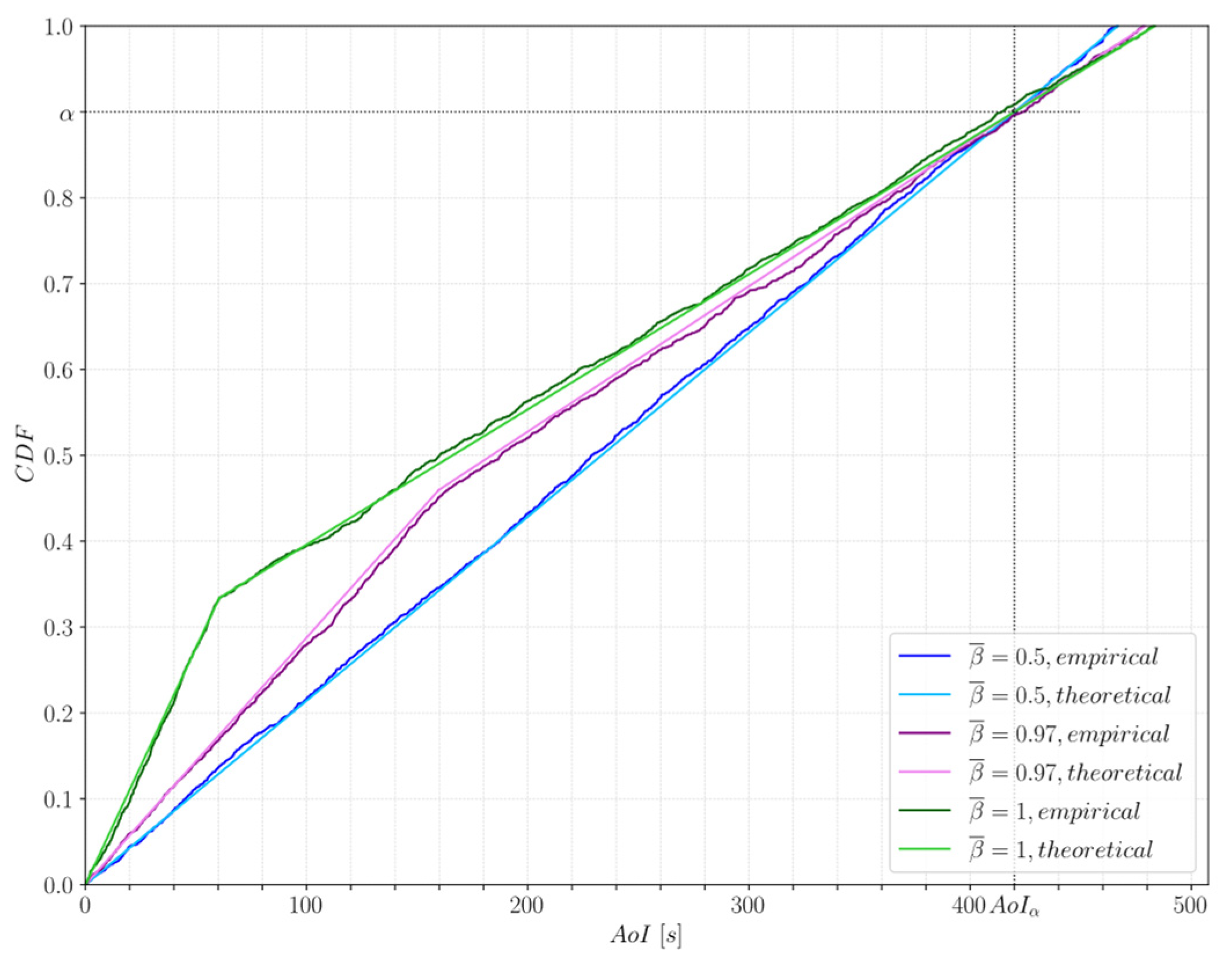
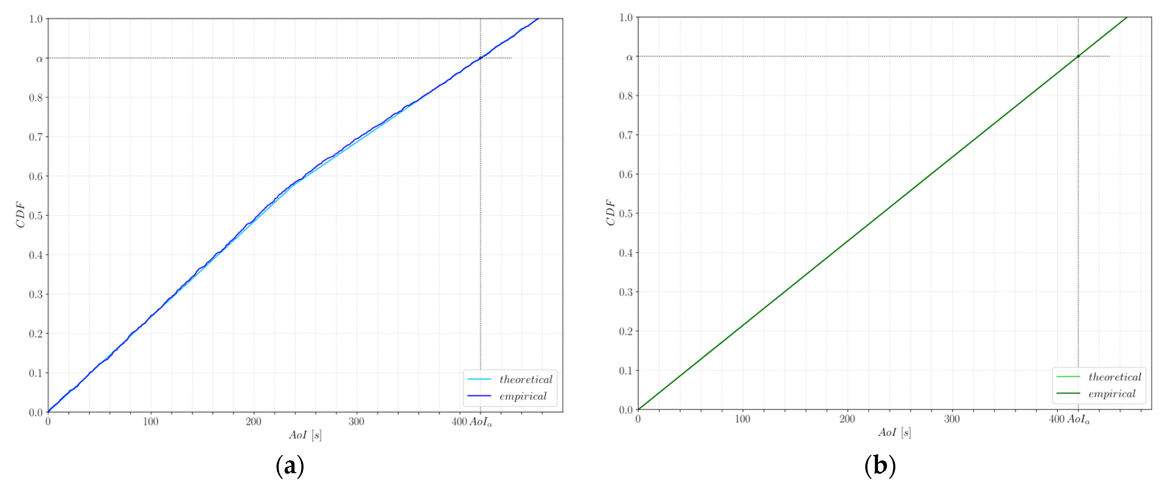
3.2.3. Probability Distribution of AoI

Denote $P_{AoI}\left(\delta W\right)$ as the probability distribution function of AoI at the steady-state. It is defined as follows:

$$P_{AoI}\left(\delta W\right)=P\left\{AoI\le \delta W|X_k=\left(1^{+},w-j\right),1\le j w\right\} \mathrm{for} \mathrm{any} \delta , 0\le \delta \le 1.$$

(4)

So:

$$P_{AoI}\left(\delta W\right)=\frac{{{\displaystyle \sum }}_{j=1}^{w}P\left\{AoI\le \delta W|X_k=\left(1^{+},w – j\right)\right\}{\pi }_{1^{+},w-j}}{{{\displaystyle \sum }}_{j=1}^w{\pi }_{1^{+},w-j}}$$

(5)

If in state $X_k=\left(1^{+},w – j\right)$ at time instant $t_k$, $1\le j\le w$, the cached sample has been collected at a time instant $t_{k-j}=t_k-js$, therefore, it is, for any $j$, $1\le j\le w$:

$$P\left\{AoI \le \delta W|X_k=\left(1^{+},w – j\right)\right\}=\{\begin{array}{c}1\\ \delta w-\lfloor \delta w\rfloor \\ 0\end{array}\begin{array}{c}j\le \lfloor \delta w\rfloor \\ \lfloor \delta w\rfloor <j\le \lfloor \delta w\rfloor +1\\ j>\lfloor \delta w\rfloor +1\end{array}$$

(6)

Finally:

$$P_{AoI}\left(\delta ws\right)=\{\begin{array}{c}\frac{\delta w}{w\left(1-e^{-\lambda s}\right)+e^{-\lambda s}} 0\le \delta <\frac{1}{w}\\ \begin{array}{c}\frac{\delta w-e^{-\lambda s}\left(\delta w-1\right)}{w\left(1-e^{-\lambda s}\right)+e^{-\lambda s}} \frac{1}{w}\le \delta \le 1\end{array}\end{array}$$

(7)

3.3. Model of the Power Consumption

Devices consume energy when performing three main tasks [30]: (i) data sampling, e.g., sensing from the environment, for example, the temperature, the humidity, the pressure, the fluid flow, etc.; (ii) data processing, performed after sampling and involving operations like storage, denoising, etc.; (iii) data communication, which includes all necessary networking tasks like packet transmissions and receptions, protocol overheads due to control traffic, etc.

We model the energy consumption as depending on two components: (i) sampling energy consumption, due to the sensing operation and the processing of the sampled data; (ii) communication energy consumption, due to the transmission of the updates. The computational energy cost can be considered negligible, as it becomes significant only in some specific cases involving complex mathematical operations or very long sleep times. Denote $c_T$ as the energy consumption for transmitting an update message and denote $c_S$ as the energy consumption for generating a new sample. The energy consumption of the device depends on the frequency of these two operations, i.e., on the transmission frequency and on the sampling frequency.

In our system model, the transmissions frequency, that we denote as $f_T,$ is the poll frequency, i.e., it is the inverse of the average time between two requests that trigger a cache refresh: $f_T\left(w,s\right)=1/E\left\{T\right\}$. The sampling frequency, that we denote as $f_S$, is instead the inverse of the sampling period: $f_S\left(w,s\right)=1/s$. So, the energy consumption per time unit $c$ on the device is

$$c=c_T{f}_T+c_S{f}_S$$

(8)

Given the wide diversity of the IoT devices, $c_T$ and $c_S$ can range from very small values to very large values, relative to each other. Without losing generality, we normalize $c$ with respect to the sum of $c_T$ and $c_S$, i.e., with respect to the sum of the energy cost of one transmission operation and the energy cost of one sampling operation:

$$\frac{c}{c_T+c_s}=\frac{c_T}{c_T+c_s}{f}_T+\frac{c_S}{c_T+c_s}{f}_S$$

(9)

Denote $c/(c_T+c_S)$ as $c_{\overline{\beta }}$, and $c_T/(c_T+c_S)$ as $\overline{\beta }$, it is:

$$c_{\overline{\beta }}=\overline{\beta }{f}_{\mathrm{T}}+\left(1-\overline{\beta }\right)f_{\mathrm{S}}$$

(10)

with $\overline{\beta }\in \left[0,1\right]$.

This means that $c_{\overline{\beta }}$ takes into account the relationship between the energy consumption of a transmission operation and a sampling operation, but it does not depend on their absolute values. Indeed, the parameter $\overline{\beta }$ indicates the energy cost of a transmission operation with respect to the sum of the energy costs of a transmission operation and a sampling operation. The value of $\overline{\beta }$ depends on the type of device, e.g., for a device where the energy cost of a sampling operation is negligible with respect to the energy cost of a transmission operation $\overline{\beta }$ tends to one; on the contrary, for a device where the energy cost of a transmission operation is negligible with respect to the energy cost of a sampling operation $\overline{\beta }$ tends to zero. In [3] Razzaque et al. compute the operational energy costs in wireless sensor networks focusing on energy consumption during a single sampling period. They consider several commercial sensors, and they present a comparison of their sensing and communication energy costs. Comparisons are normalized with respect to communication energy. In

Table 1. Exemplary values of $\overline{\beta }$ computed from commercial-sensors parameters [3].

Sensor	${\mathit{c}}_{\mathit{S}}/{\mathit{c}}_{\mathit{T}}$	$\overline{\mathit{\beta }}$
MMA7269Q (Accelerometer)	0.0000268	0.97
GE/Telaire 6004 (CO2 sensor)	1249.25	0.0008
SHT1X (H) (Humidity sensor)	0.4	0.71
SHT1X (T) (Temperature sensor)	1.5	0.4
CP 18 (Proximity sensor)	0.267	0.8
LUC-M10 (Level sensor)	9.22	0.098

we report the results for six exemplary sensors for which we compute the corresponding value of $\overline{\beta }$ starting from the given values of $c_S/c_T$. Clearly, for sensors where the cost of a sensing operation is much higher than the cost of a transmission, the value of $\overline{\beta }$ is close to zero; instead, for sensors where the cost of transmission is much higher than the cost of a sampling operation, the value of $\overline{\beta }$ is close to one.

4. Model-Driven Cache-Management Optimization

4.1. Energy-Optimized Cache Refresh

We propose a model-driven method to choose the two parameters $w$ and $s$ that minimize $c_{\overline{\beta }}$, under the constraint given by the AoI requirement. More in detail, $w$ and $s$ are the solutions to the following optimization problem:

$$mi{n}_{w,s} c_{\overline{\beta }}$$

s.t.

$$s\ge s_{min}$$

(11)

$$P_{AoI}\left(Ao{I}_{\alpha }\right)\le \alpha$$

(12)

The constraint (11) is the hardware constraint of the device, while the constraint (12) is the AoI requirement of the application. The latter can be expressed in a solvable form using our proposed model. Indeed, since the model allows us to compute the closed form of the probability distribution function, we can derive a condition on $w$ such that the probability distribution function goes through the point $\left(Ao{I}_{\alpha },y\right)$, with $y\ge \alpha$. So, we need to find $\delta$, $s,$ and $w$ such that $Ao{I}_{\alpha }=\delta W$ and $P_{AoI}\left(\delta W\right)\ge \alpha$. We obtain:

• If $1\le \delta w\le w$ (i.e., $s\le Ao{I}_{\alpha }\le W):$

  $$w\le \frac{Ao{I}_{\alpha }}{\alpha s}+\frac{e^{-\lambda s}\left(1-\alpha \right)}{\left(1-e^{-\lambda s}\right)\alpha }$$

  (13)
• If $0\le \delta w<1$ (i.e., $0\le Ao{I}_{\alpha }<s$):

  $$w\le \frac{\frac{Ao{I}_{\alpha }}{\alpha s}-{ e}^{-\lambda s}}{1-e^{-\lambda s}}$$

  (14)

Therefore, $g\left(s\right)\le w\le h\left(s\right)$, with:

$$h\left(s\right)=\{\begin{array}{c}{h}_1\left(s\right)=\frac{Ao{I}_{\alpha }}{\alpha s}+\frac{e^{-\lambda s}\left(1-\alpha \right)}{\left(1-e^{-\lambda s}\right)\alpha } s\le {AoI}_{\alpha } \\ h_2\left(s\right)=\frac{\frac{Ao{I}_{\alpha }}{\alpha s}-e^{-\lambda s}}{1-e^{-\lambda s}} s>{AoI}_{\alpha } \end{array}$$

(15)

and

$$g\left(s\right)=\frac{Ao{I}_{\alpha }}{s}.$$

(16)

An example of the feasible region where values of $w$ and $s$ satisfying the AoI requirement must fall is shown in Figure 3. Note that, although the region is highlighted as a two-dimensional area, the admissible solutions are only those on the segments for which $w$ takes an integer value.

Finally, the optimization problem can be reformulated as follows:

$$\begin{array}{c}mi{n}_{w,s} {\mathrm{c}}_{\overline{\beta }}\end{array}$$

(17)

s.t.

$$s\ge s_{min}$$

$$g\left(s\right)\le w\le h\left(s\right)$$

$$w\in {\mathbb{Z}}^{+}, s\in {ℝ}^{+}.$$

In Figure 4 we show the values of $c_{\overline{\beta }}$ inside the feasible region for different types of sensors, expressed by different values of $\overline{\beta }$. For clarity, in the figure we reported the values of $c_{\overline{\beta }}$ for all the pairs of values of $w$ and $s$ inside the feasible region; however, the only admissible pairs are those having $w\in {\mathbb{Z}}^{+}$. We can notice that for $\overline{\beta }=0$ (the energy consumption for transmitting is zero, i.e., $c_T=0$) the minimum value of $c_{\overline{\beta }}$ is on the lower right corner of the feasible region; as $\overline{\beta }$ increases, the minimum value starts shifting on the left, up to the top left corner of the feasible region when $\overline{\beta }=1$ (the energy consumption for sampling is zero, i.e., $c_S=0$). In the following, we study the objective function for the extreme cases of a device for which the energy consumption for transmitting is zero and a device for which the energy consumption for sampling is zero, having respectively, $\overline{\beta }=0$, $\overline{\beta }=1$, and then for the general case of $0<\overline{\beta }<1$, representing hybrid sensors.

4.1.1. Devices with Transmission Energy Consumption Equal to Zero: $\overline{\beta }=0$

When $\overline{\beta }=0$, i.e., $c_{\overline{\beta }}=f_{\mathrm{S}}$, it is possible to compute the optimum values of $w$ and $s$ in closed form (see Appendix A), obtaining $w^{*}=1$ and $s^{*}=Ao{I}_{\alpha }/\alpha$, as can be also seen in Figure 4. Since $c_{\overline{\beta }}=f_{\mathrm{S}}$, it follows that $c_{\overline{\beta }}$ does not depend on the rate of requests $\lambda$, but depends only on the AoI requirement, i.e., $Ao{I}_{\alpha }$ and $\alpha$.

When the value of $Ao{I}_{\alpha }$ increases, the optimum value of $c_{\overline{\beta }}$ decreases, and when $Ao{I}_{\alpha }\to \infty$, the objective function tends to 0:

$$\underset{Ao{I}_{\alpha }\to +\infty }{\lim }{f}_{\mathrm{S}}\left(\overline{s},\overline{w}\right)=0$$

Indeed, if $Ao{I}_{\alpha }\to \infty$, there is no need for refreshing the data.

When the value of $\alpha$ decreases the optimum value of $c_{\overline{\beta }}$ decreases as well, whereas when $\alpha \to 0$, the objective function tends to 0:

$$\underset{\mathsf{\alpha }\to 0}{\lim }{f}_{\mathrm{S}}\left(\overline{s},\overline{w}\right)=0$$

Indeed, $\alpha \to 0$ means that the fraction of requests that need to receive a data item whose AoI is not larger than the target value tends to zero. However, typical real use cases will require higher values of $\alpha$, e.g., 0.8, 0.9, or 0.95.

4.1.2. Devices with Sampling Energy Consumption Equal to Zero: $\overline{\beta }=1$

When $\overline{\beta }=1$, i.e., $c_{\overline{\beta }}=f_{\mathrm{T}}$, if we remove the integer constraint on $w$, it is possible to compute the optimum values of $w$ and $s$ in closed form (see Appendix B), obtaining $s^{*}=s_{min}$ and $w^{*}=f\left(s_{min}\right)=\frac{Ao{I}_{\alpha }}{\alpha s_{min}}+\frac{e^{-\lambda s_{min}}\left(1-\alpha \right)}{\left(1-e^{-\lambda s_{min}}\right)\alpha } \mathrm{if} s\le Ao{I}_{\alpha }$, or $w^{*}=f\left(s_{min}\right)=\frac{\frac{Ao{I}_{\alpha }}{\alpha s_{min}}-e^{-\lambda s_{min}}}{1-e^{-\lambda s_{min}}}\mathrm{if} s>Ao{I}_{\alpha }$. The same result can be also seen graphically in Figure 4.

In this case, $c_{\overline{\beta }}$ depends both on the requests rate $\lambda$ and on the AoI requirement, i.e., $Ao{I}_{\alpha }$ and $\alpha$.

When the value of $\lambda$ decreases, the optimum value of $c_{\overline{\beta }}$ decreases (see Figure 5), and when $\lambda \to 0$ it is:

$$\underset{\lambda \to 0}{\lim }{f}_T\left(\overline{s},\overline{w}\right)=0$$

Indeed, in this case, each request triggers a refresh with a high probability, but since the request rate is extremely low, only a few messages are exchanged in the network.

Instead, when $\lambda \to \infty$, it is (see Figure 5):

$$\underset{\lambda \to +\infty }{\lim }{f}_{\mathrm{T}}\left(\overline{s},\overline{w}\right)=\frac{\alpha }{Ao{I}_{\alpha }}$$

In this case, the cache is refreshed almost periodically with period $W$.

Clearly, also in this case, when the value of $Ao{I}_{\alpha }$ increases, the optimum value of $c_{\overline{\beta }}$ decreases, and when $Ao{I}_{\alpha }\to \infty$, the objective function tends to 0:

$$\underset{Ao{I}_{\alpha }\to +\infty }{\lim }{f}_{\mathrm{T}}\left(\overline{s},\overline{w}\right)=0$$

And when the value of $\alpha$ decreases also the optimum value of $c_{\overline{\beta }}$ decreases, and when $\alpha \to 0$, the objective function tends to 0:

$$\underset{\mathsf{\alpha }\to 0}{\lim } f_T\left(\overline{s},\overline{w}\right)=0$$

These conclusions remain essentially the same when considering the integer constraint on $w$: in this case, we cannot compute the optimum values of $w$ and $s$ in closed form, but we can only find a numerical solution using some optimization techniques and, as we can observe from Figure 6, the optimal value of $s$ can be slightly greater than $s_{min}$ to satisfy the integer constraint on $w$.

4.1.3. Hybrid Sensors: $0<\overline{\beta }<1$

In this case, both the energy consumption of transmissions and the energy consumption of sensing are different from zero, and therefore there is a trade-off between minimizing the average poll frequency and minimizing the sampling frequency on the device, as the first leads to minimizing $s$. Indeed the optimization problem chooses $s\to s_{min}$, whereas the second leads to maximize $s$.

It is possible to compute the optimum values of $w$ and $s$ solving (17) using optimization techniques for non-linear integer programming, e.g., branch and bound.

Table 2. Optimum values of $w$ and $s$ for $\lambda =1∕90 {\mathrm{s}}^{-1}$, $\lambda =1∕180{ \mathrm{s}}^{-1}$, and $\lambda =1∕360{ \mathrm{s}}^{-1}$ $\alpha =0.9$, $Ao{I}_{\alpha }=420 \mathrm{s}$, varying $\overline{\beta }$.

$\mathit{\lambda }$	$\overline{\mathit{\beta }}$	0	0.9	0.91	0.966	0.97	0.98	0.99	1
$1∕90{ \mathrm{s}}^{-1}$	$w$	1	1	1	2	3	4	6	7
	$s$	466.67	466.67	466.67	234.37	156.79	117.88	78.82	67.63
$1∕180{ \mathrm{s}}^{-1}$	$w$	1	1	2	3	3	4	5	8
	$s$	466.67	466.67	238.14	159.7	159.7	120.18	96.36	60.44
$1∕360{ \mathrm{s}}^{-1}$	$w$	1	2	2	2	3	3	4	8
	$s$	466.67	247.25	247.25	247.25	166.05	166.05	125.03	62.91

and Figure 6 show the optimum values of $w$ and $s$ computed using the APMonitor solver ([31,32]) using $\alpha =0.9$, $Ao{I}_{\alpha }=420 \mathrm{s}$, and considering three exemplary cases where $\lambda =1∕90{ \mathrm{s}}^{-1}$, $\lambda =1∕180{ \mathrm{s}}^{-1}$ and $\lambda =1∕360{ \mathrm{s}}^{-1}$. We can notice that the optimum values are on the top edge of the feasible region, as in the cases shown in Figure 4. Moreover, we can also notice that several values of $\overline{\beta }$ can result in the same configuration of the parameters $w$ and $s$: Table 2 shows that in all the considered scenarios, there are different values of $\overline{\beta }$, i.e., different types of devices, that have the same optimum values of $w$ and $s$. This follows from the model constraint that $w$ can only take integer values. However, the resulting values of $c_{\overline{\beta }}$ are different as they depend on the value of $\overline{\beta }$, i.e., the energy consumption still depends on the type of device.

Figure 7 shows $c_{\overline{\beta }}$ for different types of devices and for the same AoI requirement and five possible network loads: $\lambda =1∕10{ \mathrm{s}}^{-1}$, $\lambda =1∕180{ \mathrm{s}}^{-1}$, $\lambda =1∕500{ \mathrm{s}}^{-1}$, $\lambda =1∕1000{ \mathrm{s}}^{-1}$ and $\lambda =1∕1800{ \mathrm{s}}^{-1}$. Clearly, as the request rate decreases also the transmission energy cost decreases. As mentioned above, in all the considered scenarios for values of $\overline{\beta }$ going from 0 up to 0.9-0.91-0.97, the optimum values of $w$ and $s$ are the same, hence their values of $c_{\overline{\beta }}$ differ only for $\overline{\beta }$, showing a linear behavior. Instead, when $\overline{\beta }\to 1$ the optimum values of $w$ and $s$ change and, at lower rates we also have that $f_{\mathrm{T}}\to 0$, so $c_{\overline{\beta }}\to 0$, causing the steep change in the slope of the curve.

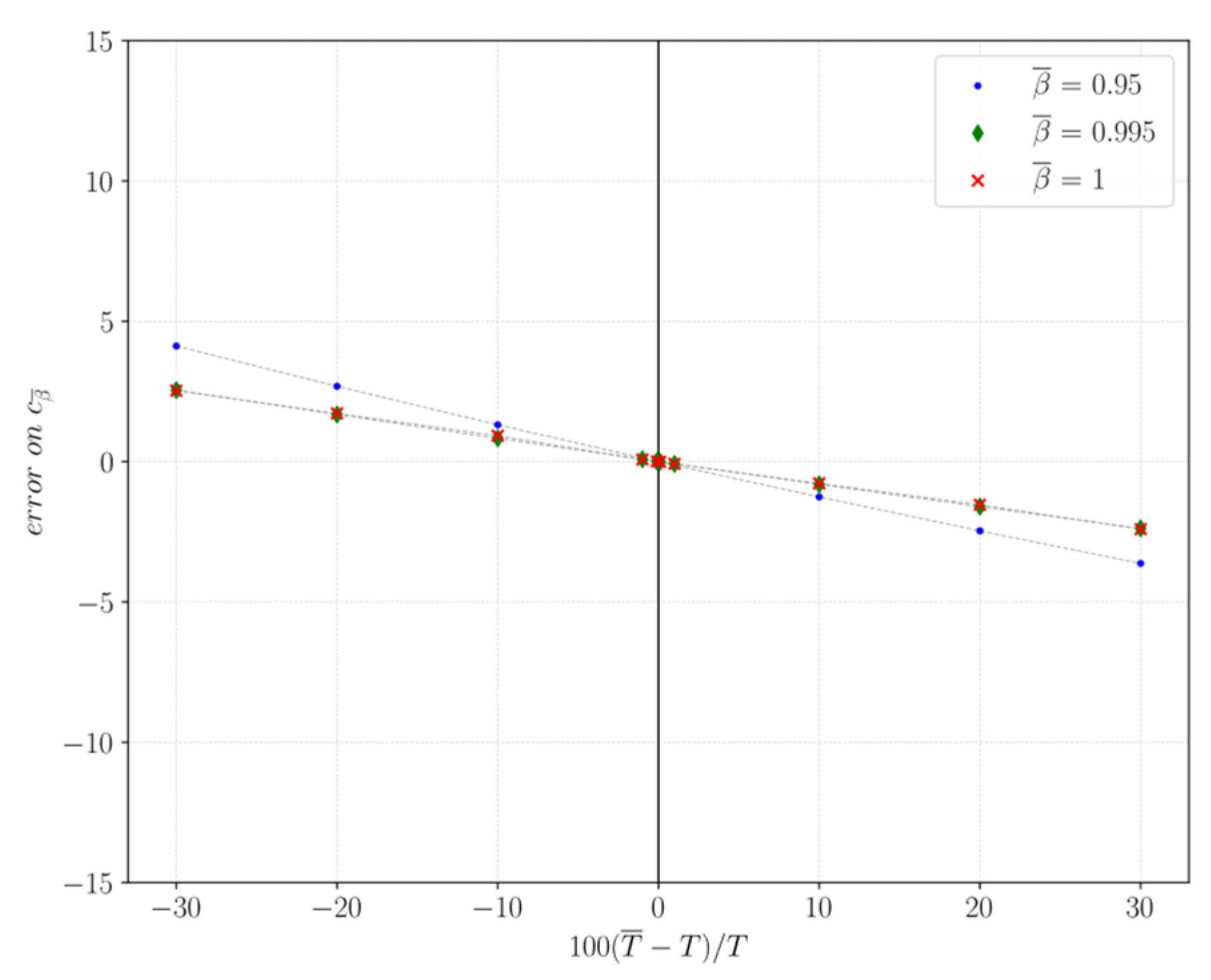
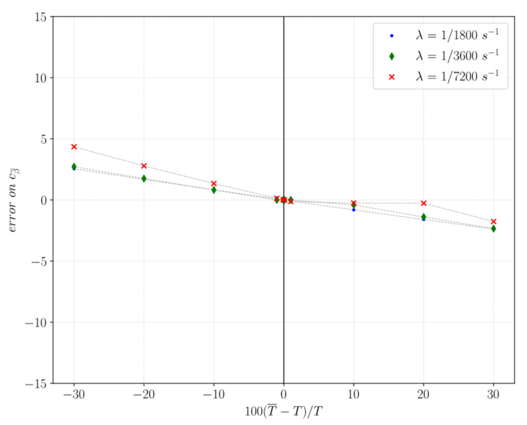
4.2. Sensitivity Analysis

The cache optimizer needs to receive as inputs the AoI requirements of the application, i.e., $\alpha$ and $Ao{I}_{\alpha }$, and the request rate $\lambda$. The proxy receives the values of $\alpha$ and $Ao{I}_{\alpha }$ from the server during the initial configuration phase; instead, it needs to estimate the value of the request rate $\lambda$. So, the estimated value of $\lambda$ may be affected by an estimation error, or the actual value of $\lambda$ may not be constant but have some small fluctuations that are not seen by the proxy.

To assess the sensitivity of the proposed model to variations of the parameter $\lambda$, we evaluate our model in a sample scenario in which we assume that the AoI requirements are $\alpha =0.9$ and $Ao{I}_{\alpha }=420 \mathrm{s}$, for different values of $\overline{\beta }$ and $\lambda$. Typically, estimating the rate of a Poisson process requires estimating the mean interarrival time; so, in the following, we show the sensitivity of our model when the estimated mean interarrival time, denoted as $\overline{T}$, is different from the actual mean interarrival time, denoted as $T$. Since we want to evaluate the impact of an estimation error of $T$, we are considering devices where the predominant energy cost is the transmission energy cost, i.e., $\overline{\beta }\to 1$: indeed, in these cases $c_{\overline{\beta }}$ also depends on the request rate and hence is more affected by estimation errors on $T$.

Call $w^{*}$ and $s^{*}$ the optimum values obtained considering the mean interarrival time $T$ and call $\overline{w}$ and $\overline{s}$ the optimum values obtained considering the estimated interarrival time $\overline{T}$. Figure 8 shows the percentage variation of $c_{\overline{\beta }}$, calculated as follows:

$$\frac{c_{\overline{\beta }}\left(T, \overline{w}, \overline{s}\right) – c_{\overline{\beta }}\left(T, w^{*}, s^{*}\right)}{c_{\overline{\beta }}\left(T, w^{*}, s^{*}\right)}\ast 100$$

(18)

as a function of the percentage variation of $T$, i.e., $100\left(\overline{T}-T\right)/T$. Moreover, call ${\pi }_{\alpha }$ the $\alpha$-th percentile of $P_{AoI}$. Figure 9 shows the percentage variation of ${\pi }_{\alpha }$, calculated as follows:

$$\frac{{\pi }_{\alpha }\left(T, \overline{w}, \overline{s}\right) – {\pi }_{\alpha }\left(T, w^{*}, s^{*}\right)}{{\pi }_{\alpha }\left(T, w^{*}, s^{*}\right)}\ast 100$$

(19)

as a function of the percentage variation of $T$.

From Figure 8 we can notice that when $T$ is underestimated, the resulting energy consumption cost is larger than the minimum value, though the variation is small. On the other hand, when $T$ is overestimated, the energy consumption is smaller, but the AoI requirement is not satisfied (see Figure 9). However, for small variations of $T$, the percentage variation of ${\pi }_{\alpha }$ is small.

Finally, Figure 10 shows the percentage variation of $c_{\overline{\beta }}$ for different values of $\lambda =1/T$. We can notice that lower rates are more affected by estimation errors, because as $\lambda$ tends to zero, also the transmission energy cost tends to zero, and hence larger errors on $T$ have a larger impact on $c_{\overline{\beta }}$. However, the graphs show that the model is robust, indeed if we assume that $T$ varies up to 30%, in the worst case the error is slightly more than 10%.

5. Performance Evaluation

Exemplary Use Case: LWM2M

IoT devices generate complex and heterogeneous M2M systems that need to be configured, monitored, and maintained, so there is a need for a standard platform for management. For example, the Open Mobile Alliance (OMA) specified the LightweightM2M (LWM2M) protocol for device management and service enablement. LWM2M defines an application layer protocol between an LWM2M Server, i.e., the IoT application, and the LWM2M Client, i.e., the IoT device. It is designed for constrained devices and networks and provides a set of REST-based resource models where each information made available by the device is a Resource. Resources are then organized into Objects. This object model is easily extensible, and the Object registry is open to the industry. So, LWM2M is becoming broadly used in industry: in this context, the IIoT network manager aims at reducing the energy consumption in the device to prolong its lifetime and reduce the operating costs of the network while satisfying the AoI requirements of the applications. Hence, a possible solution is using a caching system at the edge.

To assess the performance of our solution in this use case, we emulate an IoT system where we use the LWM2M protocol to manage the IoT devices and we consider a scenario consisting of an IoT network, an LWM2M Server that runs the IoT application and a cache-enabled LWM2M Proxy that implements our proposed cache-management scheme.

The IoT network is emulated using the COOJA network emulator [33] and uses the 6LoWPAN protocol [34] on top of the IEEE 802.15.4 MAC [35] operating in the 2.4 GHz band, and the RPL routing protocol [36]. The wireless devices of the IoT network run the Contiki-NG operating system [37] and are connected to the Internet through the 6LoWPAN Border Router. One of the devices runs the LWM2M Client, that in this case is the device application, exposing an LWM2M Object representing the sensor, and is located three hops away from the 6LoWPAN Border Router. The LWM2M Proxy is located outside the IoT network and manages the requests for the device application sent by the IoT application using the proposed cache-management scheme. The LWM2M Server and the LWM2M Proxy are implemented using the Eclipse Leshan library [38]. Each experiment lasted 400,000 s, the frame size of a response message is 82 bytes and the resulting average service delay, i.e., the time between when a request is issued by the application and the time its response is received, is 326.5 ms (95% CI [322.6, 330.4]), and it is negligible compared to the chosen value of $Ao{I}_{\alpha }$, i.e., $420 \mathrm{s}$.

In our first experiment, $\alpha$ is $0.9$ and the generation of application-requests follows a Poisson distribution with a cumulative rate $\lambda =1∕180{ \mathrm{s}}^{-1}$(as in the examples shown in Section 4.1.3). Figure 11 shows the empirical CDFs and the CDFs obtained through the model for the following values of $\overline{\beta }$: $\overline{\beta }=0.5$, $\overline{\beta }=0.97$, $\overline{\beta }=1$.

Table 3. $w$ , $s$, and $\overline{AoI}$ for $\lambda =1∕180 s^{-1}$, $\alpha =0.9$, $Ao{I}_{\alpha }=420 s$, varying $\overline{\beta }$.

$\overline{\mathit{\beta }}$	0.5	0.97	1
$w$	1	3	8
$s$	466.67	159.7	60.44
$\overline{AoI}$	231.53 95% CI [221.93, 241.16]	212.31 95% CI [203.51, 221.11]	189.98 95% CI [182.08, 197.88]

shows the values of $w$ and $s$ chosen by the optimizer. We can see that the empirical and the theoretical results are very close to each other, so the empirical CDFs obtained with the values of $w$ and $s$ chosen by the model always satisfy the AoI requirements. Moreover, Table 3 also shows the values of $\overline{AoI}$ in all the considered cases: we can notice the trade-off between minimizing the average poll frequency and minimizing the sampling frequency, indeed when $\overline{\beta }=1$, it is $s\to s_{min}$, that results in a lower value of $\overline{AoI}$, but this comes at the cost of a higher sampling power consumption.

In our second experiment, we consider the same configuration as the previous experiment, but now multiple IoT applications send periodic requests for the state of the IoT device. We consider two cases: (i) in the first scenario, ten applications have request periods of the same order of magnitude, e.g., the applications have similar characteristics, and so all the request periods are randomly extracted from a uniform distribution between 1000 and 3000 s; (ii) in the second scenario, five applications have periods uniformly distributed between 50 and 100 s, while the remaining five have periods uniformly distributed between 5000 and 10,000 s, e.g., we consider two different classes of applications. In the first scenario, we consider $\overline{\beta }=0.95$, in the second scenario we assume $\overline{\beta }=1$. The optimizer computes the optimum values using $\lambda$ as the sum of the inverses of the periods and chooses (i) $w=2$ and $s=238.1 \mathrm{s}$ for the first scenario and (ii) $w=7$ and $s=66.68 \mathrm{s}$ for the second scenario. Figure 12 shows the empirical CDFs and the CDFs obtained through the model for the two scenarios: we can notice that the empirical CDFs and the theoretical CDFs are very close to each other, so the optimum values of $w$ and $s$ obtained through the model can be applied also in this case.

To assess the performance of the cache implemented by the proxy, we compare the case in which the proxy implements the cache against the case in which the proxy does not implement the cache. In the latter case, we consider $s=Ao{I}_{\alpha }/\alpha$, i.e., the maximum value of $s$ that satisfies the AoI constraint. In Figure 13 we report the value of $c_{\overline{\beta }}$ obtained for different types of devices both without the cache and with the cache. We can notice that the optimized cache can significantly reduce the energy cost of devices for which the cost of the transmissions is the prevalent cost because it can significantly reduce the number of transmissions, especially for high values of $\lambda$. We can also notice that using the cache makes the system less sensitive to higher rates, as the number of exchanged messages depends on the refresh window.

Then, we define the service delay as the time between a request sent by the application and the time its response is received. Figure 14 shows the cumulative distribution function of the service delay for $\lambda =1/180{\mathrm{s}}^{-1}$ both for the case in which the proxy does not implement the cache and for the case wherein the proxy implements the cache. For the latter, we consider three values of $\overline{\beta }$, namely $\overline{\beta }=0.5$, $\overline{\beta }=0.97$ and $\overline{\beta }=1$. All the scenarios satisfy the same AoI requirements: $Ao{I}_{\alpha }=420 \mathrm{s}$ and $\alpha =0.9$. Clearly, we can notice that the cache-enabled proxy always provides quicker responses with respect to the case in which the cache is not implemented, as some responses are taken from the cache, as shown by the CDFs. Indeed, the CDFs obtained with the cache show a bi-modal behavior: some responses are taken from the cache and hence have smaller service delays, while some responses are forwarded to the device and hence have larger service delays. Moreover, we can also notice that the case $\overline{\beta }=1$ is the configuration that minimizes the service delay. Indeed, $\overline{\beta }=1$ is the case in which the predominant energy cost is the transmission cost, so it minimizes the number of exchanged messages with the device and hence it is also the configuration that minimizes the service delay.

6. Conclusions

In this work, we considered an IoT network composed of devices that sample the environment periodically and of applications that need to be aware of the state of these devices as timely as possible to, for example, support decision making or detect anomalies. However, the timeliness of the state updates is limited by the constraints of the IoT devices and networks, especially by the device energy constraints. Indeed, energy is a scarce resource, as typically devices do not have a fixed power supply, but they rely on batteries or harvest energy. The energy consumption of the device mainly depends on the sensing energy consumption and on the transmission energy consumption; so, the objective of IoT-system management is to minimize them while guaranteeing information freshness. Indeed, minimizing the energy consumption of devices can reduce the operating costs of the network, as it prolongs a device’s lifetime. A possible method is using a caching system because it can help in reducing sensing frequency and transmission frequency. Typically, IoT networks are accessed through gateways/proxies that act as intermediaries between devices and applications. Usually, these gateways/proxies are also used to provide a better system performance, e.g., they implement a cache to lower the energy consumption on the device. Hence, several cache refreshing schemes have been proposed in the literature that minimizes freshness and energy consumption or balance freshness and service latency. We instead minimize the energy consumption on the device and consider the freshness of the data, measured by AoI, as a constraint in terms of percentile of the distribution, because typically applications establish a threshold on the value of the AoI. So, we considered a cache-enabled proxy deployed at the edge in between devices and applications: it receives the requests for status updates of a device from an application and responds using its cached item or, if the cached item is expired, it fetches the last update from the device, refreshes the cache, and delivers it to the application. The freshness of a cached item is quantified using the AoI metrics, and a cached item is no longer considered fresh when its AoI exceeds the value of the cache parameter denoted as refresh window, W. In a preliminary version of this work [10], we proposed a model for this cache management scheme. In this work, we leverage that model to define and solve an optimization problem that configures the cache parameter W to minimize the energy consumption on the device, which depends on the average poll frequency and on the sampling frequency, while satisfying an AoI constraint expressed by the application. We apply our proposed cache-enabled proxy in two different emulated IoT scenarios that use the LWM2M protocol for device management: in the first one, requests are generated according to a Poisson distribution, while in the second one requests are periodic. Results show that our proposed solution minimizes energy consumption while satisfying the AoI requirements.

Moreover, this per-device cache uses a simple yet effective management scheme that does not pose any limitation on the number of applications issuing requests on the device and that has constant complexity, i.e., it only involves a comparison between the AoI of the cached item and its refresh window. So, our solution can be easily applied in deployments involving multiple IoT devices just scaling vertically, i.e., adding more resources to the proxy, or scaling horizontally, i.e., replicating the proxy.

In future work, we aim to consider also different cache refreshing policies, e.g., the cache could be updated using observing streams from the device.

References

1. Huang, H.; Qiao, D.; Gursoy, M.C. Age-Energy Tradeoff Optimization for Packet Delivery in Fading Channels. IEEE Trans. Wirel. Commun. 2021, 21, 179–190. [Google Scholar] [CrossRef]
2. Zhou, B.; Saad, W. Optimal Sampling and Updating for Minimizing Age of Information in the Internet of Things. In Proceedings of the 2018 IEEE Global Communications Conference (GLOBECOM), Abu Dhabi, United Arab Emirates, 9–13 December 2018; pp. 1–6. [Google Scholar]
3. Razzaque, M.A.; Dobson, S. Energy-efficient sensing in wireless sensor networks using compressed sensing. Sensors 2014, 14, 2822–2859. [Google Scholar] [CrossRef] [PubMed] [Green Version]
4. Kim-Hung, L.; Le-Trung, Q. User-Driven Adaptive Sampling for Massive Internet of Things. IEEE Access 2020, 8, 135798–135810. [Google Scholar] [CrossRef]
5. Zhong, J.; Yates, R.D.; Soljanin, E. Two Freshness Metrics for Local Cache Refresh. In Proceedings of the 2018 IEEE International Symposium on Information Theory (ISIT), Vail, CO, USA, 17–22 June 2018; pp. 1924–1928. [Google Scholar]
6. Kaul, S.; Gruteser, M.; Rai, V.; Kenney, J. Minimizing Age of Information in Vehicular Networks. In Proceedings of the 2011 8th Annual IEEE Communications Society Conference on Sensor, Mesh and Ad Hoc Communications and Networks, Salt Lake City, UT, USA, 27–30 June 2011; pp. 350–358. [Google Scholar]
7. Yates, R.D.; Sun, Y.; Brown, D.R.; Kaul, S.K.; Modiano, E.; Ulukus, S. Age of information: An introduction and survey. IEEE J. Sel. Areas Commun. 2021, 39, 1183–1210. [Google Scholar] [CrossRef]
8. Kosta, A.; Pappas, N.; Angelakis, V. Age of information: A new concept, metric, and tool. Found. Trends Netw. 2017, 12, 162–259. [Google Scholar] [CrossRef] [Green Version]
9. Costa, M.; Codreanu, M.; Ephremides, A. On the age of information in status update systems with packet management. IEEE Trans. Inf. Theory 2016, 62, 1897–1910. [Google Scholar] [CrossRef]
10. Pappalardo, M.; Mingozzi, E.; Virdis, A. A Model-Driven Approach to Aol-Based Cache Management in IoT. In Proceedings of the 2021 IEEE 26th International Workshop on Computer Aided Modeling and Design of Communication Links and Networks (CAMAD), Porto, Portugal, 25–27 October 2021; pp. 1–6. [Google Scholar]
11. Pappalardo, M.; Virdis, A.; Mingozzi, E. An Edge-Based LWM2M Proxy for Device Management to Efficiently Support QoS-Aware IoT Services. IoT 2022, 3, 169–190. [Google Scholar] [CrossRef]
12. Open Mobile Alliance. Lightweight Machine to Machine Technical Specification: Core; Open Mobile Alliance: San Diego, CA, USA, 2020. [Google Scholar]
13. Open Mobile Alliance. Lightweight Machine to Machine Technical Specification: Transport Bindings; Open Mobile Alliance: San Diego, CA, USA, 2020. [Google Scholar]
14. Chen, Z.; Sivaparthipan, C.B.; Muthu, B. IoT based smart and intelligent smart city energy optimization. Sustain. Energy Technol. Assess. 2022, 49, 101724. [Google Scholar] [CrossRef]
15. Naeem, A.; Javed, A.R.; Rizwan, M.; Abbas, S.; Lin, J.C.-W.; Gadekallu, T.R. DARE-SEP: A Hybrid Approach of Distance Aware Residual Energy-Efficient SEP for WSN. IEEE Trans. Green Commun. Netw. 2021, 5, 611–621. [Google Scholar] [CrossRef]
16. Dev, K.; Maddikunta, P.K.R.; Gadekallu, T.R.; Bhattacharya, S.; Hegde, P.; Singh, S. Energy optimization for green communication in IoT using harris hawks optimization. IEEE Trans. Green Commun. Netw. 2022, 6, 685–694. [Google Scholar] [CrossRef]
17. Abbas, Q.; Hassan, S.A.; Pervaiz, H.; Ni, Q. A Markovian Model for the Analysis of Age of Information in IoT Networks. IEEE Wirel. Commun. Lett. 2021, 10, 1596–1600. [Google Scholar] [CrossRef]
18. Akar, N.; Dogan, O. Discrete-Time Queueing Model of Age of Information with Multiple Information Sources. IEEE Internet Things J. 2021, 8, 14531–14542. [Google Scholar] [CrossRef]
19. Kaul, S.; Yates, R.; Gruteser, M. Real-Time Status: How Often Should One Update? In Proceedings of the 2012 Proceedings IEEE INFOCOM, Orlando, FL, USA, 25–30 March 2012; pp. 2731–2735. [Google Scholar]
20. Abd-Elmagid, M.A.; Pappas, N.; Dhillon, H.S. On the role of age of information in the Internet of Things. IEEE Commun. Mag. 2019, 57, 72–77. [Google Scholar] [CrossRef] [Green Version]
21. Chiariotti, F.; Holm, J.; Kalør, A.E.; Soret, B.; Jensen, S.K.; Pedersen, T.B.; Popovski, P. Query Age of Information: Freshness in Pull-Based Communication. IEEE Trans. Commun. 2022, 70, 1606–1622. [Google Scholar] [CrossRef]
22. Niyato, D.; Kim, D.I.; Wang, P.; Song, L. A Novel Caching Mechanism for Internet of Things (IoT) Sensing Service with Energy Harvesting. In Proceedings of the 2016 IEEE International Conference on Communications (ICC), Kuala Lumpur, Malaysia, 23–27 May 2016; pp. 1–6. [Google Scholar]
23. Xu, C.; Wang, X.; Yang, H.H.; Sun, H.; Quek, T.Q. AoI and Energy Consumption Oriented Dynamic Status Updating in Caching Enabled IoT Networks. In Proceedings of the IEEE INFOCOM 2020—IEEE Conference on Computer Communications Workshops (INFOCOM WKSHPS), Toronto, ON, Canada, 6–9 July 2020; pp. 710–715. [Google Scholar]
24. Zhang, S.; Li, J.; Luo, H.; Gao, J.; Zhao, L.; Shen, X.S. Low-Latency and Fresh Content Provision in Information-Centric Vehicular Networks. IEEE Trans. Mobile Comput. 2020, 21, 1723–1738. [Google Scholar] [CrossRef]
25. Zhang, S.; Li, J.; Luo, H.; Gao, J.; Zhao, L.; Shen, X.S. Towards fresh and low-latency content delivery in vehicular networks: An edge caching aspect. In Proceedings of the 2018 10th International Conference on Wireless Communications and Signal Processing (WCSP), Hangzhou, China, 18–20 October 2018; pp. 1–6. [Google Scholar]
26. Zhang, S.; Wang, L.; Luo, H.; Ma, X.; Zhou, S. AoI-delay tradeoff in mobile edge caching with freshness-aware content refreshing. IEEE Trans. Wirel. Commun. 2021, 20, 5329–5342. [Google Scholar] [CrossRef]
27. Mezair, T.; Djenouri, Y.; Belhadi, A.; Srivastava, G.; Lin, J.C.-W. Towards an Advanced Deep Learning for the Internet of Behaviors: Application to Connected Vehicle. Available online: https://dl.acm.org/doi/abs/10.1145/3526192 (accessed on 23 June 2022).
28. Taivalsaari, A.; Mikkonen, T. A roadmap to the programmable world: Software challenges in the IoT era. IEEE Softw. 2017, 34, 72–80. [Google Scholar] [CrossRef]
29. Li, C.; Li, S.; Hou, Y.T. A general model for minimizing age of information at network edge. In Proceedings of the IEEE INFOCOM 2019—IEEE Conference on Computer Communications, Paris, France, 29 April–2 May 2019; pp. 118–126. [Google Scholar]
30. Fragkiadakis, A.; Charalampidis, P.; Tragos, E. Adaptive compressive sensing for energy efficient smart objects in IoT applications. In Proceedings of the 2014 4th International Conference on Wireless Communications, Vehicular Technology, Information Theory and Aerospace & Electronic Systems (VITAE), Aalborg, Denmark, 11–14 May 2014; pp. 1–5. [Google Scholar]
31. Hedengren, J.D.; Asgharzadeh Shishavan, R.; Powell, K.M.; Edgar, T.F. Nonlinear Modeling, Estimation and Predictive Control in APMonitor. Comput. Chem. Eng. 2014, 70, 133–148. [Google Scholar] [CrossRef] [Green Version]
32. Beal, L.D.R.; Hill, D.; Martin, R.A.; Hedengren, J.D. GEKKO Optimization Suite. Processes 2018, 8, 106. [Google Scholar] [CrossRef] [Green Version]
33. Available online: https://github.com/contiki-ng/cooja (accessed on 3 June 2022).
34. Available online: https://datatracker.ietf.org/wg/6lowpan/documents/ (accessed on 3 June 2022).
35. IEEE Std 802.15.4-2015; IEEE Standard for Low-RateWireless Networks. IEEE: Piscataway Township, NJ, USA, 2016.
36. Winter, T.; Thubert, P.; Brandt, A.; Hui, J.; Kelsey, R.; Levis, P.; Pister, K.; Struik, R.; Vasseur, J.P.; Alexander, R. RPL: IPv6 Routing Protocol for Low-Power and Lossy Networks; RFC 6550; IETF: Fremont, CA, USA, 2012. [Google Scholar]
37. Available online: https://github.com/contiki-ng/contiki-ng (accessed on 3 June 2022).
38. Available online: https://github.com/eclipse/leshan (accessed on 3 June 2022).
Figure 1. IoT system overview and model: (a) a typical IoT system, (b) the considered scenario, (c) the interplay over time between the arrival process of IoT-application requests, the sampling process, and the cache operations.
Futureinternet 14 00197 g001
Figure 2. Discrete Time Markov Chain.
Futureinternet 14 00197 g002
Figure 3. Constraints for A o I α = 420   s , α = 0.9 , λ = 1 1800   s 1 and s m i n = 60   s (log scale on the y-axis).
Futureinternet 14 00197 g003
Figure 4. Values of c β ¯ for A o I α = 420   s , α = 0.9 , λ = 1 1800   s 1 , and s m i n = 60   s , varying β ¯ : (a) β ¯ = 0 , (b) β ¯ = 0.994 , (c) β ¯ = 0.997 , (d) β ¯ = 1 (log scale on the y-axis).
Futureinternet 14 00197 g004
Figure 5. Values of c β ¯   for β ¯ = 1 , varying λ and A o I α .
Futureinternet 14 00197 g005
Figure 6. Optimum values of w and s for (a) λ = 1 90   s 1 , (b) λ = 1 180   s 1 , and (c) λ = 1 360   s 1   α = 0.9 , A o I α = 420   s , varying β ¯ .
Futureinternet 14 00197 g006
Figure 7. c β ¯ for α = 0.9 , A o I α = 420   s , λ = 1 10   s 1 , λ = 1 180   s 1 , λ = 1 500   s 1 , λ = 1 1000   s 1 , and λ = 1 1800   s 1 .
Futureinternet 14 00197 g007
Figure 8. Percentage variation of the normalized energy cost for λ = 1 1800   s 1 , β ¯ = 0.95 (circles), β ¯ = 0.995 (diamonds), β ¯ = 1 (crosses).
Futureinternet 14 00197 g008
Figure 9. Percentage variation of A o I α for λ = 1 1800   s 1 , β ¯ = 0.95 (circles), β ¯ = 0.995 (diamonds), β ¯ = 1 (crosses).
Futureinternet 14 00197 g009
Figure 10. Percentage variation of the cost: λ = 1 1800   s 1 (circles), λ = 1 3600   s 1 (diamonds), λ = 1 7200   s 1 (crosses), β ¯ = 0.995 .
Futureinternet 14 00197 g010
Figure 11. Theoretical AoI CDF and empirical AoI CDF for λ = 1 180   s 1 , α = 0.9 , A o I α = 420   s .
Futureinternet 14 00197 g011
Figure 12. AoI CDF with 10 periodic servers: (a) first scenario, (b) second scenario.
Futureinternet 14 00197 g012
Figure 13. c β ¯ for α = 0.9 , A o I α = 420   s , λ = 1 360   s 1 , λ = 1 180   s 1 , and λ = 1 90   s 1 .
Futureinternet 14 00197 g013
Figure 14. Service delay for λ = 1 180   s 1 .
Futureinternet 14 00197 g014