
Positioning Energy-Neutral Devices: Technological Status and Hybrid RF-Acoustic Experiments


Abstract
:
1. Introduction
- A comprehensive overview on the up-to-date state of the art of indoor positioning technologies.
- A discussion of different hybrid RF-acoustic systems zooming in on methods to achieve the positioning of energy-neutral devices.
- Presentation and analysis of ranging experiments demonstrating the opportunities and open challenges to accurate 3D positioning.
2. Preliminaries and State of the Art
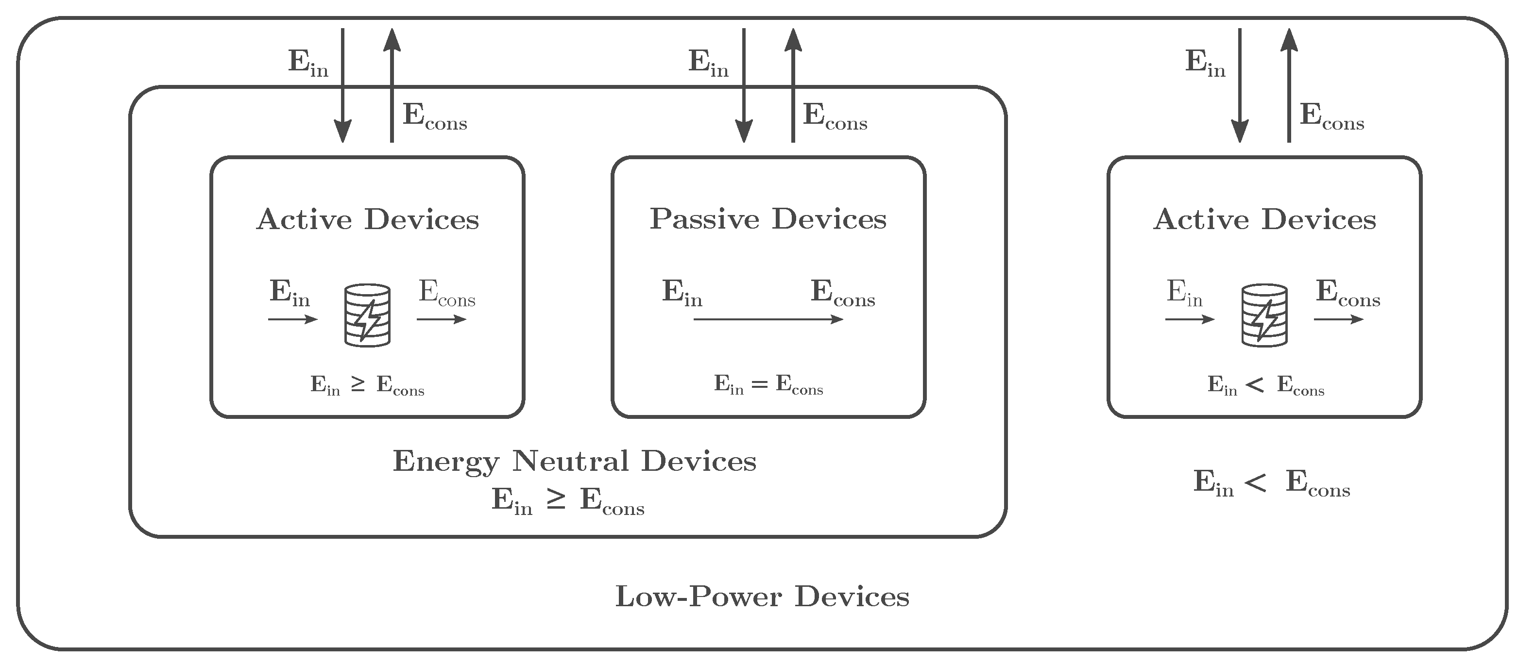
2.1. Interacting with Ultra-Low Power and Energy-Neutral Devices
2.2. Indoor Positioning Technologies
3. Hybrid Acoustic-RF Approaches for Positioning Energy-Neutral Devices
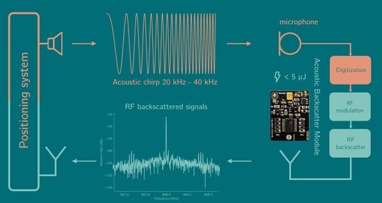
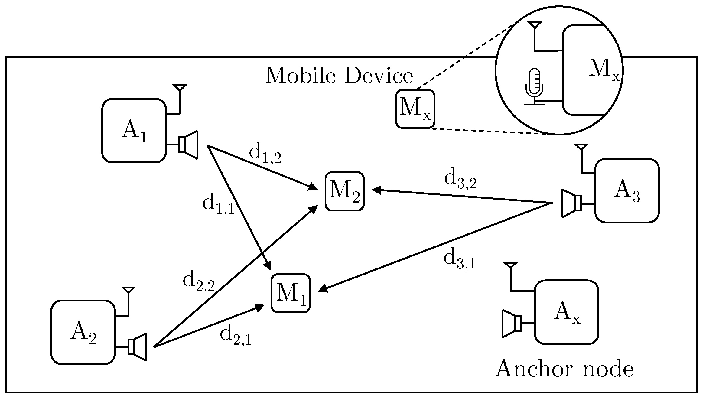
3.1. Setup
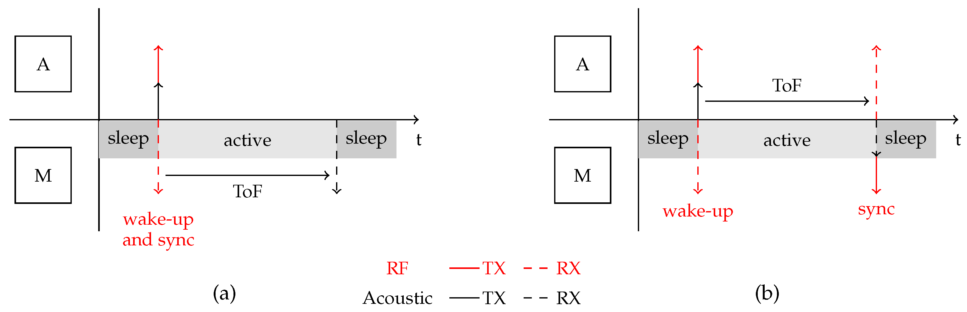
3.2. Signaling
3.3. RF Backscattering
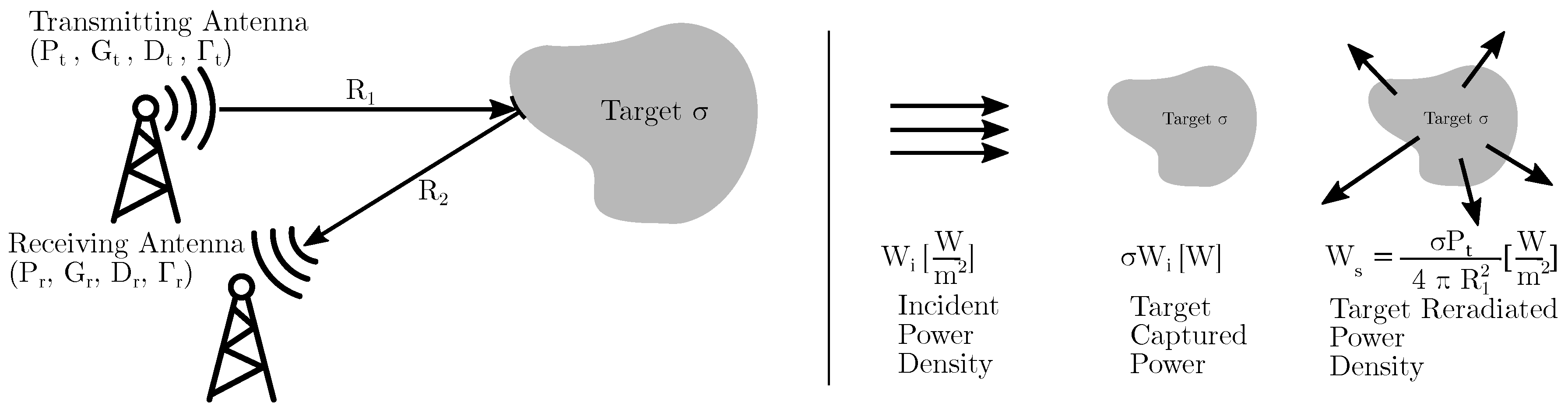
3.3.1. Antenna Scattering
3.3.2. Backscatter Modulation
3.4. Hardware Implementation, Power Consumption and Backscatter Demodulation
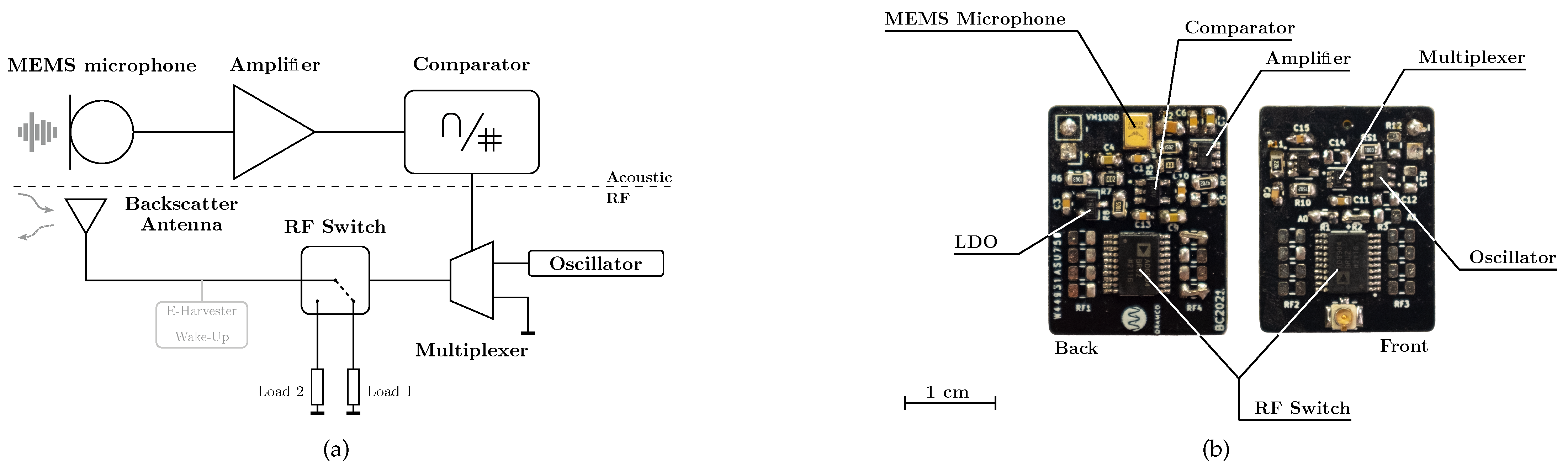
3.4.1. Hardware Implementation and Power Review
- MEMS microphone (Vesper VM1000): key specifications in addition to its low-power consumption include its short wake-up time (below 200 µs), high sensitivity, and wide frequency response. In-house measurements show that frequencies over 80 kHz can be received sufficiently, much higher than stated in the audible domain-focused datasheet (Note that this frequency range is true for the tested microphone’s batch. No guarantee can be given that other future batches of this microphone type will behave similarly).
- Amplifier (TI TLV341): this low-noise amplifier has a high UGB, providing a gain up to 34.8 dB for a 40 kHz signal in a single stage. Amplifying and filtering before zero-crossing by the comparator is more noise resilient and therefore gives better results. The single-supply rail-to-rail capability of this opamp makes for an easy implementation and for maximum signal amplitude swings.
- Comparator (TI TLV7031): the rise and fall time are specified below 5 nanoseconds, giving a quasi-instant change of state when a zero-crossing occurs.
3.4.2. Backscatter Demodulation
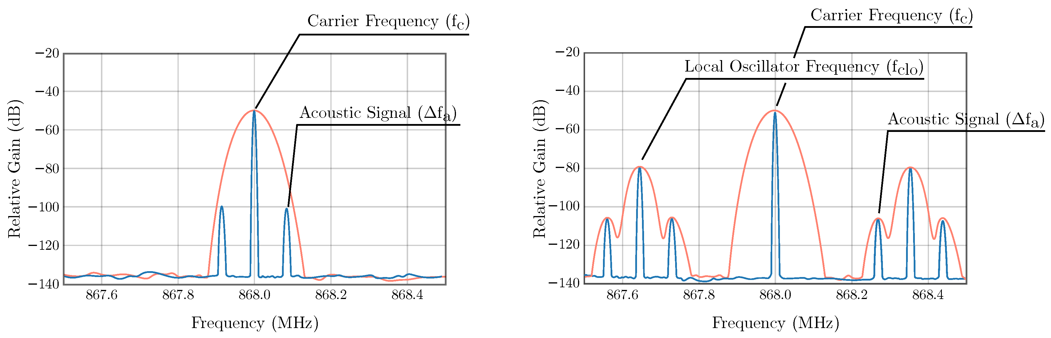
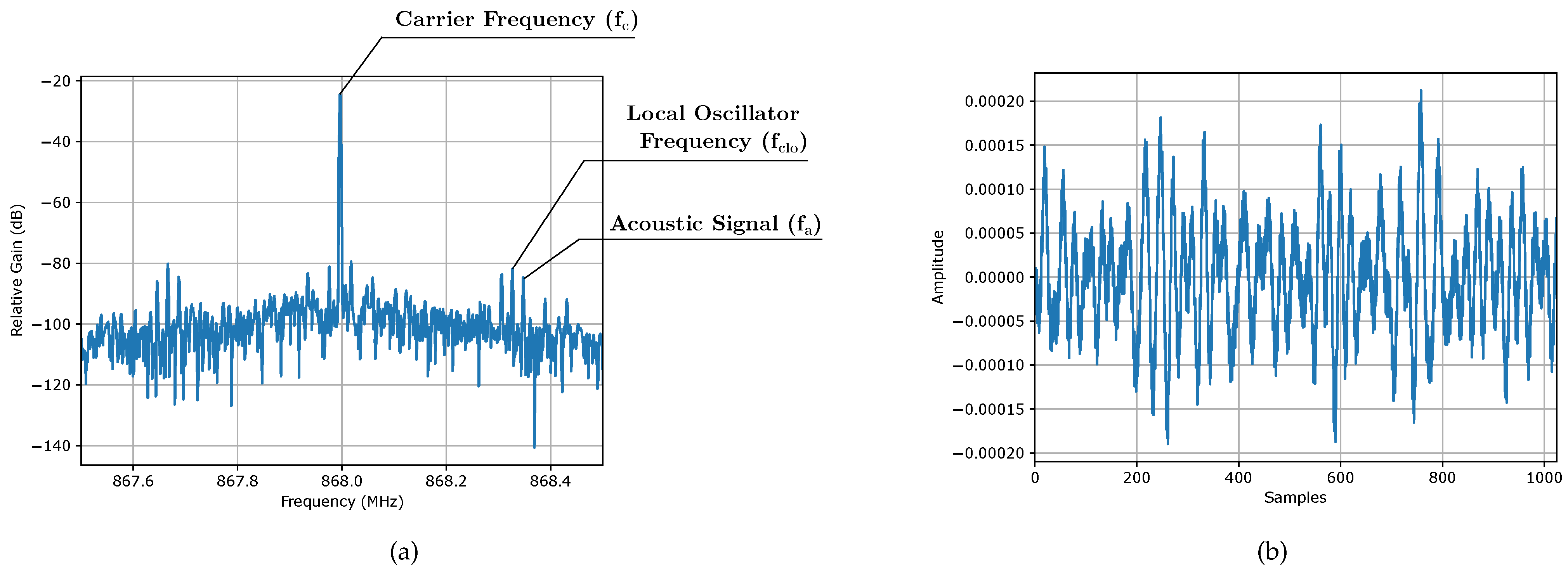
- OOK demodulation. The digitized acoustic signal drives a multiplexer that forwards either the local oscillator or no signal at all. Consequently, the load is switched at the local oscillator frequency or it is not switched. In the spectrum, this appears as a signal away from the RF carrier frequency that is turned on and off. As mentioned previously, OOK is very susceptible to noise, and the drift of the local oscillators can make the amplitude demodulation on the receiving radio impossible.
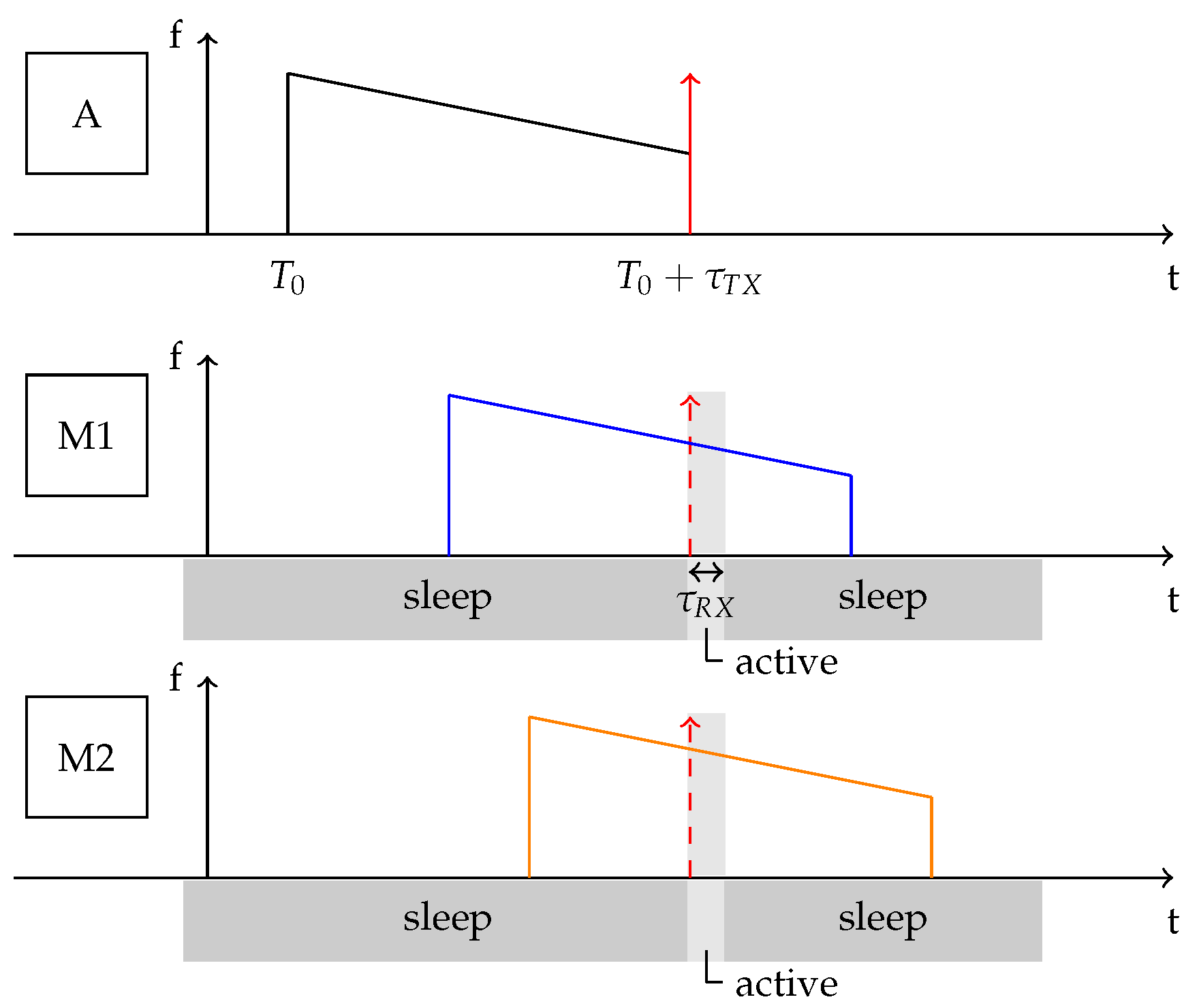
- FSK demodulation. As the acoustic chirp can be considered as a signal modulated in frequency, this chirp signal can be observed on both sides of the local oscillator frequency. The demodulation is done by performing a frequency translation and a decimating FIR filter on one of the sidebands. With this, only the portion of the wideband signal with the frequency decreasing chirp signal is saved to a buffer for later use.
4. Experiments Demonstrating Opportunities and Challenges in Hybrid RF-Acoustic Positioning
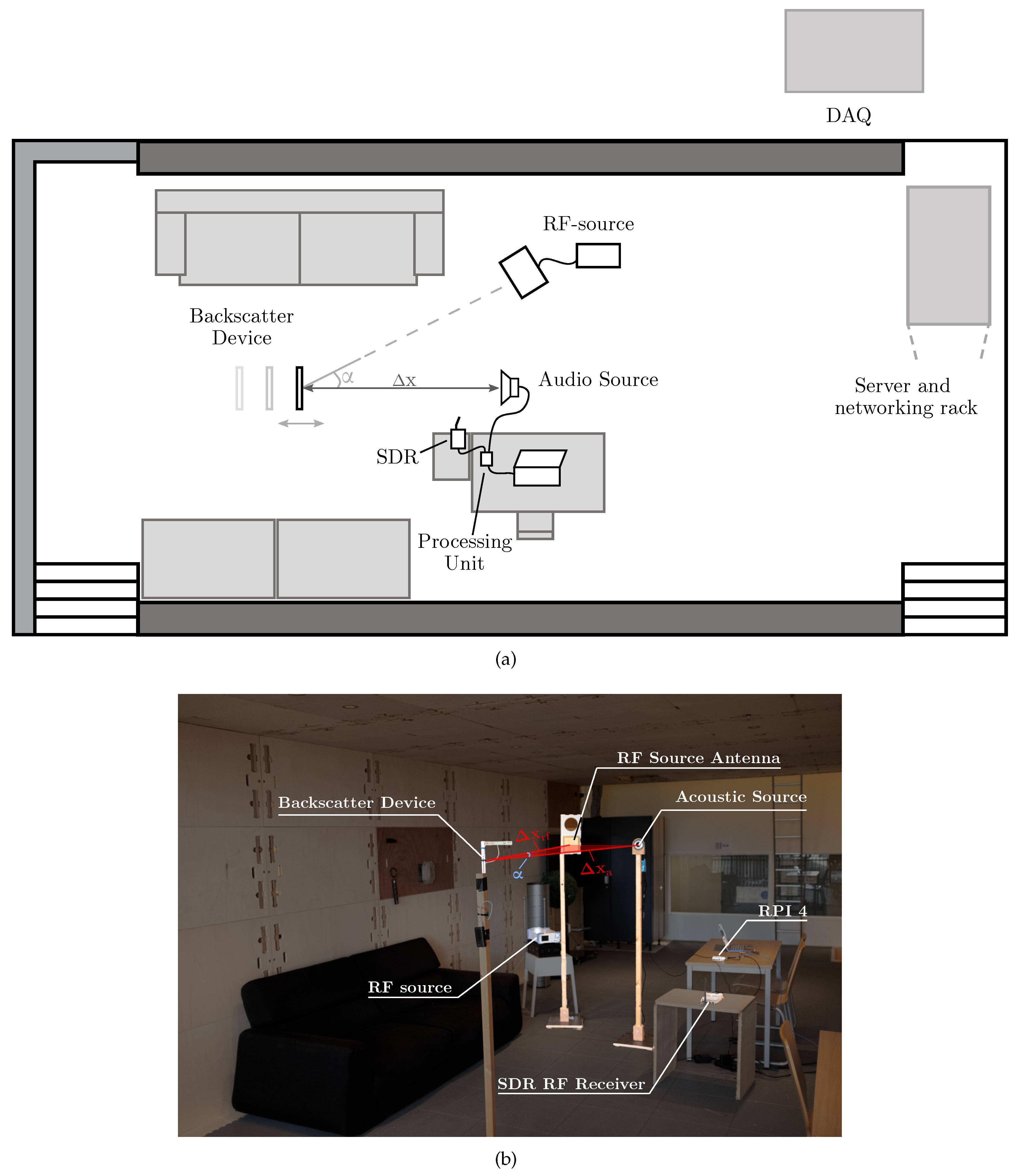
4.1. Experimental Environment and Measurement Setup
- RF source: a single frequency carrier sine wave of 868 MHz with an output power of 12 dBm is sent out by R&S SMC100a signal generator. A directional patch antenna with a 6.15 dBi gain is attached to this setup, contributing to a total output power of 18.15 dBm, well below the 27 dBm EIRP upper limit imposed by the ETSI regulations. The antenna is mounted on a pole, at the same height as the antenna of the backscatter device.
- Processing unit for audio transmission (@anchor node): The acoustic signal is generated on a Raspberry Pi 4 running a Debian-based operating system. A C library PiGPIO is used for sending out the chirp with a frequency between 40 kHz and 20 kHz by binary switching a GPIO pin for 30 ms. The audio signal is amplified with an off-the-shelf amplifier with a frequency range over 45 kHz. The audio signals are transmitted by a Fostex FT17H ultrasonic tweeter with a HPBW below 30° in the xy-plane at 25 kHz. Similar to the RF source, the speaker is mounted on a pole and directed towards the MEMS microphone of the backscatter device.
- Backscatter device (@mobile device): Consists of both RF and audio components and was detailed in Section 3.4.
- Processing unit with SDR (@anchor node): The same Raspberry Pi 4 is used as processing unit running Python-based GNU radio in parallel with custom C++ timing and an acoustic signal-generating code. The RF backscattered waves were received by a dipole antenna connected to an Ettus B210 USRP SDR, and converted, filtered, and handled by signal-processing blocks in GNU radio. These FM-demodulated signals are stored in the hard drive for further distance range calculations. Interrupt-based precise timing between the start-up of the acoustic chirp and the RF wake-up time is performed by the software as well, with a maximum measured offset of 10 µs.
4.2. Conducted Experiments
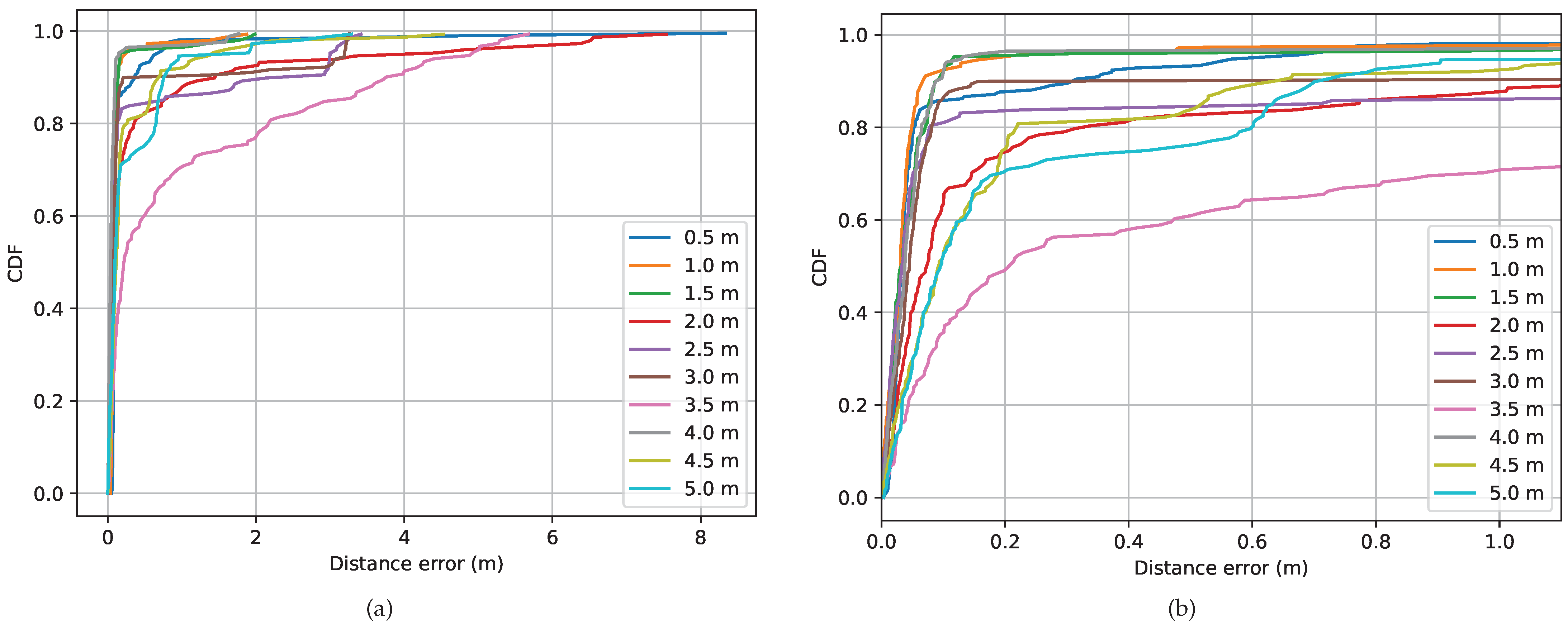
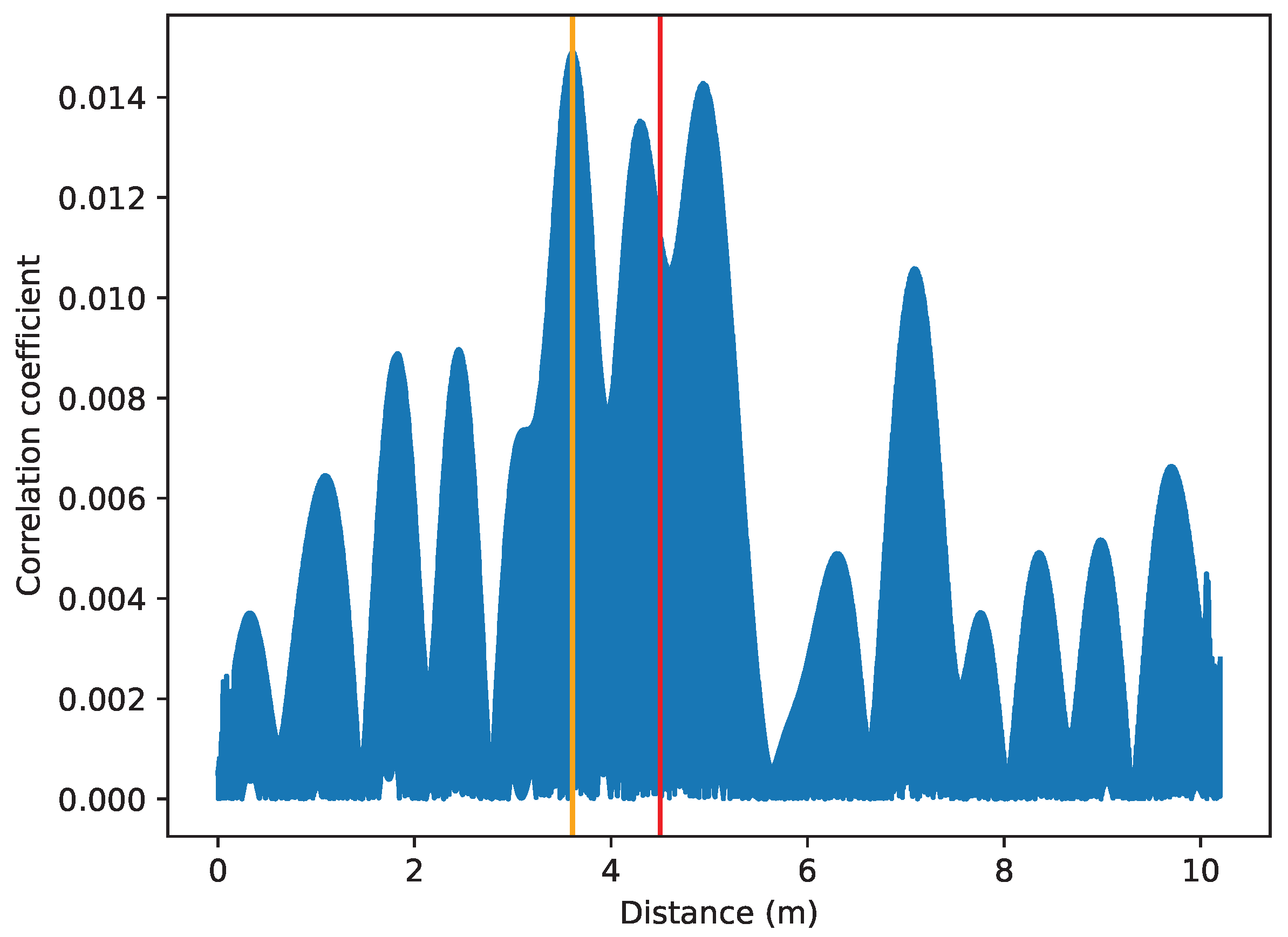
4.2.1. Ranging Audio
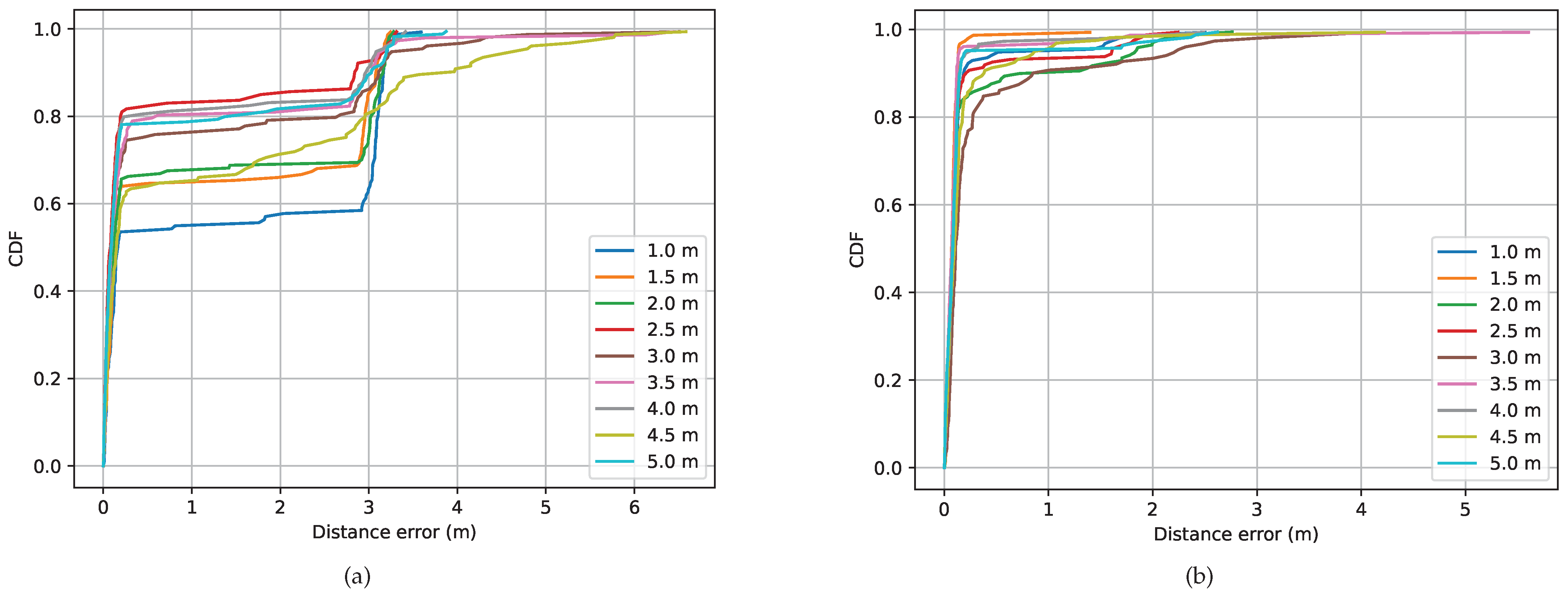
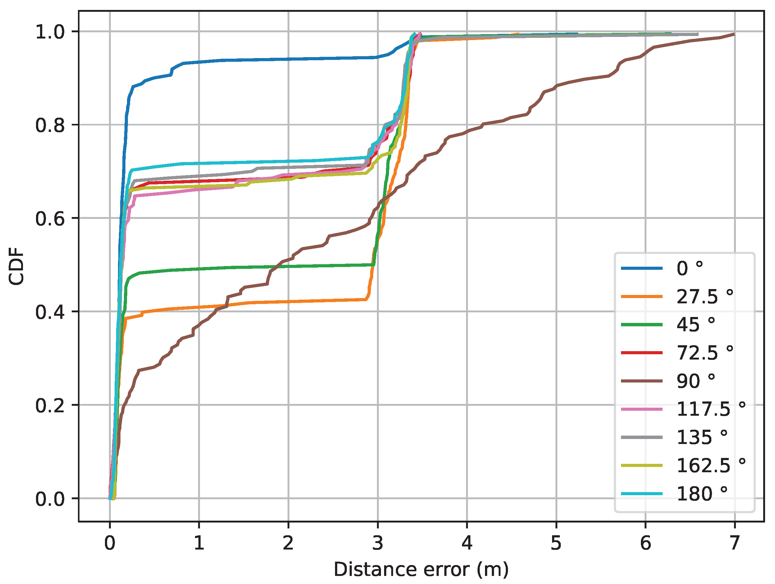
4.2.2. Ranging-RF
5. Conclusions and Road Ahead
Author Contributions
Funding
Data Availability Statement
Conflicts of Interest
Abbreviations
| DAQ | data acquisition system |
| PoE | power-over-Ethernet |
| USRP | universal software radio peripheral |
| MEMS | micro-electro-mechanical system |
| ADC | analog-to-digital converter |
| DAC | digital-to-analog converter |
| FS | full scale |
| RFPT | radio frequency power transmission |
| SoC | system on chip |
| SDR | software-defined radio |
| LIDAR | laser imaging detection and ranging |
| DDS | direct digital synthesis |
| RT | reverberation time |
| RTA | real-time analyzer |
| SPL | sound pressure level |
| TP | test point |
| TDoA | time difference of arrival |
| SLAM | simultaneous localization and mapping |
| PTP | precision time protocol |
| NLoS | non-line of sight |
| WPT | wireless power transfer |
| RF | radio frequency |
| LOS | line of sight |
| EIRP | effective isotropic radiated power |
| HPBW | half power beam width |
| APT | acoustic power transfer |
| IoT | Internet of Things |
| RSSI | received signal strength indicator |
| UWB | ultra wideband |
| PoA | phase of arrival |
| ToF | time of flight |
| RFID | radio-frequency identification |
| CDF | cumulative distribution function |
| MIMO | multiple-input–multiple-output |
| STMR | side lobe-to-main lobe ratio |
| PCB | printed circuit board |
| RCS | radar cross-section |
| OOK | on–off keying |
| ASK | amplitude shift keying |
| FSK | frequency shift keying |
| IC | integrated circuit |
| UGB | unity gain bandwidth |
| CMUT | capacitive micro-machined ultrasonic transducers |
| FMDA | frequency division multiple access |
| LDO | low dropout |
| SOTA | state of the art |
| RT60 | reverberation time (60 dB) |
References
- Adu-Manu, K.S.; Adam, N.; Tapparello, C.; Ayatollahi, H.; Heinzelman, W. Energy-Harvesting Wireless Sensor Networks (EH-WSNs): A Review. ACM Trans. Sen. Netw. 2018, 14, 1–50. [Google Scholar] [CrossRef]
- Magno, M.; Aoudia, F.A.; Gautier, M.; Berder, O.; Benini, L. WULoRa: An energy efficient IoT end-node for energy harvesting and heterogeneous communication. In Proceedings of the Design, Automation Test in Europe Conference Exhibition (DATE), Lausanne, Switzerland, 27–31 March 2017; pp. 1528–1533. [Google Scholar]
- La Rosa, R.; Livreri, P.; Trigona, C.; Di Donato, L.; Sorbello, G. Strategies and Techniques for Powering Wireless Sensor Nodes through Energy Harvesting and Wireless Power Transfer. Sensors 2019, 19, 2660. [Google Scholar] [CrossRef] [PubMed] [Green Version]
- Awal, M.R.; Jusoh, M.; Sabapathy, T.; Kamarudin, M.R.; Rahim, R.A. State-of-the-Art Developments of Acoustic Energy Transfer. Int. J. Antennas Propag. 2016, 2016, 1–14. [Google Scholar] [CrossRef] [Green Version]
- Cansiz, M.; Altinel, D.; Kurt, G.K. Efficiency in RF energy harvesting systems: A comprehensive review. Energy 2019, 174, 292–309. [Google Scholar] [CrossRef]
- Oguntala, G.; Abd-Alhameed, R.; Jones, S.; Noras, J.; Patwary, M.; Rodriguez, J. Indoor location identification technologies for real-time IoT-based applications: An inclusive survey. Comput. Sci. Rev. 2018, 30, 55–79. [Google Scholar] [CrossRef]
- Cadena, C.; Carlone, L.; Carrillo, H.; Latif, Y.; Scaramuzza, D.; Neira, J.; Reid, I.; Leonard, J.J. Past, Present, and Future of Simultaneous Localization and Mapping: Toward the Robust-Perception Age. IEEE Trans. Robot. 2016, 32, 1309–1332. [Google Scholar] [CrossRef] [Green Version]
- Tahat, A.; Kaddoum, G.; Yousefi, S.; Valaee, S.; Gagnon, F. A Look at the Recent Wireless Positioning Techniques With a Focus on Algorithms for Moving Receivers. IEEE Access 2016, 4, 6652–6680. [Google Scholar] [CrossRef]
- He, S.; Chan, S.H.G. Wi-Fi Fingerprint-Based Indoor Positioning: Recent Advances and Comparisons. IEEE Commun. Surv. Tutorials 2016, 18, 466–490. [Google Scholar] [CrossRef]
- Witrisal, K.; Hinteregger, S.; Kulmer, J.; Leitinger, E.; Meissner, P. High-accuracy positioning for indoor applications: RFID, UWB, 5G, and beyond. In Proceedings of the 2016 IEEE International Conference on RFID (RFID), Orlando, FL, USA, 3–5 May 2016; pp. 1–7. [Google Scholar]
- Gomes, E.L.; Fonseca, M.; Lazzaretti, A.E.; Munaretto, A.; Guerber, C. Clustering and Hierarchical Classification for High-Precision RFID Indoor Location Systems. IEEE Sens. J. 2022, 22, 5141–5149. [Google Scholar] [CrossRef]
- Errington, A.F.C.; Daku, B.L.F.; Prugger, A.F. Initial Position Estimation Using RFID Tags: A Least-Squares Approach. IEEE Trans. Instrum. Meas. 2010, 59, 2863–2869. [Google Scholar] [CrossRef]
- Saab, S.S.; Nakad, Z.S. A Standalone RFID Indoor Positioning System Using Passive Tags. IEEE Trans. Ind. Electron. 2011, 58, 1961–1970. [Google Scholar] [CrossRef]
- DiGiampaolo, E.; Martinelli, F. Mobile Robot Localization Using the Phase of Passive UHF RFID Signals. IEEE Trans. Ind. Electron. 2014, 61, 365–376. [Google Scholar] [CrossRef]
- Cruz, C.C.; Costa, J.R.; Fernandes, C.A. Hybrid UHF/UWB Antenna for Passive Indoor Identification and Localization Systems. IEEE Trans. Ant. Prop. 2013, 61, 354–361. [Google Scholar] [CrossRef] [Green Version]
- Zwirello, L.; Schipper, T.; Jalilvand, M.; Zwick, T. Realization Limits of Impulse-Based Localization System for Large-Scale Indoor Applications. IEEE Trans. Instrum. Meas. 2015, 64, 39–51. [Google Scholar] [CrossRef]
- Flueratoru, L.; Wehrli, S.; Magno, M.; Niculescu, D. On the Energy Consumption and Ranging Accuracy of Ultra-Wideband Physical Interfaces. In Proceedings of the GLOBECOM 2020—2020 IEEE Global Communications Conference, Taipei, Taiwan, 7–11 December 2020; pp. 1–7. [Google Scholar]
- Cruz, C.C.; Costa, J.R.; Fernandes, C.A. Design of a passive tag for indoor localization. In Proceedings of the 2012 6th European Conference on Antennas and Propagation (EUCAP), Prague, Czech Republic, 26–30 March 2012; pp. 2495–2499. [Google Scholar]
- Urena, J.; Hernandez, A.; Garcia, J.J.; Villadangos, J.M.; Carmen Perez, M.; Gualda, D.; Alvarez, F.J.; Aguilera, T. Acoustic Local Positioning With Encoded Emission Beacons. Proc. IEEE 2018, 106, 1042–1062. [Google Scholar] [CrossRef]
- Liu, M.; Cheng, L.; Qian, K.; Wang, J.; Wang, J.; Liu, Y. Indoor acoustic localization: A survey. Hum.-Centric Comput. Inf. Sci. 2020, 10, 1–24. [Google Scholar] [CrossRef]
- Qiu, Z.; Lu, Y.; Qiu, Z. Review of Ultrasonic Ranging Methods and Their Current Challenges. Micromachines 2022, 13, 520. [Google Scholar] [CrossRef]
- Medina, C.; Segura, J.C.; De la Torre, A. Ultrasound indoor positioning system based on a low-power wireless sensor network providing sub-centimeter accuracy. Sensors 2013, 13, 3501–3526. [Google Scholar] [CrossRef] [Green Version]
- Carotenuto, R.; Pezzimenti, F.; Corte, F.G.D.; Iero, D.; Merenda, M. Acoustic Simulation for Performance Evaluation of Ultrasonic Ranging Systems. Electronics 2021, 10, 1298. [Google Scholar] [CrossRef]
- Ogiso, S. Robust acoustic localization in a reverberant environment for synchronous and asynchronous beacons. In Proceedings of the 2021 International Conference on Indoor Positioning and Indoor Navigation (IPIN), Lloret de Mar, Spain, 29 November–2 December 2021; pp. 1–8. [Google Scholar]
- Carotenuto, R.; Merenda, M.; Iero, D.; Della Corte, F.G. An Indoor Ultrasonic System for Autonomous 3-D Positioning. IEEE Trans. Instrum. Meas. 2019, 68, 2507–2518. [Google Scholar] [CrossRef]
- Carotenuto, R.; Merenda, M.; Iero, D.; Corte, F.G.D. Using ANT Communications for Node Synchronization and Timing in a Wireless Ultrasonic Ranging System. IEEE Sensors Lett. 2017, 1, 1–4. [Google Scholar] [CrossRef]
- Rekhi, A.S.; So, E.; Gural, A.; Arbabian, A. CRADLE: Combined RF/Acoustic Detection and Localization of Passive Tags. IEEE Trans. Circuits Syst. I Regul. Pap. 2021, 68, 2555–2568. [Google Scholar] [CrossRef]
- Zhao, Y.; Smith, J.R. A battery-free RFID-based indoor acoustic localization platform. In Proceedings of the 2013 IEEE International Conference on RFID (RFID), Orlando, FL, USA, 30 April–2 May 2013; pp. 110–117. [Google Scholar]
- Merenda, M.; Catarinucci, L.; Colella, R.; Della Corte, F.G.; Carotenuto, R. Exploiting RFID technology for Indoor Positioning. In Proceedings of the 2021 6th International Conference on Smart and Sustainable Technologies (SpliTech), Bol and Split, Croatia, 8–11 September 2021; pp. 1–5. [Google Scholar]
- Mannay, K.; Urena, J.; Hernandez, A.; Machhout, M.; Aguili, T. 3D Ultrasonic Indoor Local Positioning System: Study and Implementation. The Convergence of 5G & Smart Computing Days 2019 (5G & SC’19). 2019. Available online: https://www.researchgate.net/profile/Khaoula-Mannay/publication/358107373_3D_Ultrasonic_Indoor_Local_Positioning_System_Study_and_Implementation/links/61f06a0c8d338833e395d921/3D-Ultrasonic-Indoor-Local-Positioning-System-Study-and-Implementation.pdf?origin=publication_detail (accessed on 4 May 2022).
- Chen, X.; Chen, Y.; Cao, S.; Zhang, L.; Zhang, X.; Chen, X. Acoustic Indoor Localization System Integrating TDMA+FDMA Transmission Scheme and Positioning Correction Technique. Sensors 2019, 19, 2353. [Google Scholar] [CrossRef] [PubMed] [Green Version]
- Cao, S.; Chen, X.; Zhang, X.; Chen, X. Effective Audio Signal Arrival Time Detection Algorithm for Realization of Robust Acoustic Indoor Positioning. IEEE Trans. Instrum. Meas. 2020, 69, 7341–7352. [Google Scholar] [CrossRef]
- Wang, J.; Zhang, M.; Wang, Z.; Sun, S.; Ning, Y.; Yang, X.; Pang, W. An Ultra-Low Power, Small Size and High Precision Indoor Localization System Based on MEMS Ultrasonic Transducer Chips. IEEE Trans. Ultrason. Ferroelectr. Freq. Control 2022, 69, 1469–1477. [Google Scholar] [CrossRef]
- Wang, J.; Sun, S.; Ning, Y.; Zhang, M.; Pang, W. Ultrasonic TDoA Indoor Localization Based on Piezoelectric Micromachined Ultrasonic Transducers. In Proceedings of the 2021 IEEE International Ultrasonics Symposium (IUS), Xi’an, China, 12–15 September 2021; pp. 1–3. [Google Scholar]
- Carotenuto, R.; Merenda, M.; Iero, D.; Corte, F.G.D. Ranging RFID Tags With Ultrasound. IEEE Sen. J. 2018, 18, 2967–2975. [Google Scholar] [CrossRef]
- Aguilera, T.; Álvarez, F.J.; Paredes, J.A.; Moreno, J.A. Doppler compensation algorithm for chirp-based acoustic local positioning systems. Digit. Signal Process. 2020, 100, 102704. [Google Scholar] [CrossRef]
- Wielandt, S.; Strycker, L.D. Indoor Multipath Assisted Angle of Arrival Localization. Sensors 2017, 17, 2522. [Google Scholar] [CrossRef] [Green Version]
- Holm, S. Hybrid ultrasound-RFID indoor positioning: Combining the best of both worlds. In Proceedings of the 2009 IEEE International Conference on RFID, Orlando, FL, USA, 27–28 April 2009; pp. 155–162. [Google Scholar]
- Zubair, A.; Tariq, Z.B.; Naqvi, I.H.; Uppal, M. SHARF: A Single Beacon Hybrid Acoustic and RF Indoor Localization Scheme. In Cognitive Radio Oriented Wireless Networks; Weichold, M., Hamdi, M., Shakir, M.Z., Abdallah, M., Karagiannidis, G.K., Ismail, M., Eds.; Springer International Publishing: Cham, Switzerland, 2015; pp. 499–510. [Google Scholar]
- Li, X.; Leitinger, E.; Oskarsson, M.; Åström, K.; Tufvesson, F. Massive MIMO-Based Localization and Mapping Exploiting Phase Information of Multipath Components. IEEE Trans. Wirel. Commun. 2019, 18, 4254–4267. [Google Scholar] [CrossRef] [Green Version]
- Cox, B.; De Strycker, L.; Van der Perre, L. Acoustic Backscatter: Enabling Ultra-Low Power, Precise Indoor Positioning. In Proceedings of the 2018 Ubiquitous Positioning, Indoor Navigation and Location-Based Services (UPINLBS), Wuhan, China, 22–23 March 2018; pp. 1–6. [Google Scholar]
- Cox, B.; Van der Perre, L.; De Strycker, L. Zero-Crossing Chirp Frequency Demodulation for Ultra-Low-Energy Precise Hybrid RF-Acoustic Ranging of Mobile Nodes. IEEE Sensors Lett. 2020, 4, 1–4. [Google Scholar] [CrossRef]
- Cox, B.; Van der Perre, L.; Wielandt, S.; Ottoy, G.; De Strycker, L. High precision hybrid RF and ultrasonic chirp-based ranging for low-power IoT nodes. EURASIP J. Wirel. Commun. Netw. 2020, 2020, 1–24. [Google Scholar] [CrossRef]
- Landt, J. The history of RFID. IEEE Potentials 2005, 24, 8–11. [Google Scholar] [CrossRef]
- Van Huynh, N.; Hoang, D.T.; Lu, X.; Niyato, D.; Wang, P.; Kim, D.I. Ambient Backscatter Communications: A Contemporary Survey. IEEE Commun. Surv. Tutor. 2018, 20, 2889–2922. [Google Scholar] [CrossRef] [Green Version]
- Kellogg, B.; Parks, A.; Gollakota, S.; Smith, J.R.; Wetherall, D. Wi-Fi Backscatter: Internet Connectivity for RF-Powered Devices. In Proceedings of the 2014 ACM Conference on SIGCOMM, SIGCOMM ’14, Chicago, IL, USA, 17–22 August 2014; Association for Computing Machinery: New York, NY, USA, 2014; pp. 607–618. [Google Scholar]
- Balanis, C.A. Antenna Theory: Analysis and Design; Wiley-Interscience: Hoboken, NJ, USA, 2005. [Google Scholar]
- Knott, E.F.; Schaeffer, J.F.; Tulley, T.M. Radar Cross Section; SciTech Publishing: Raleigh, NC, USA, 2004. [Google Scholar]
- Green, R.B. The General Theory of Antenna Scattering. Ph.D. Thesis, The Ohio State University, Columbus, OH, USA, 1963. [Google Scholar]
- Ruck, G.T.; Barrick, D.E.; Stuart, W.D.; Krichbaum, C.K. Radar cross Section Handbook; Plenum Press: New York, NY, USA, 1970. [Google Scholar]
- Hansen, R.C. Relationships between antennas as scatterers and as radiators. Proc. IEEE 1989, 77, 659–662. [Google Scholar] [CrossRef] [Green Version]
- Varshney, A.; Pérez-Penichet, C.; Rohner, C.; Voigt, T. LoRea: A Backscatter Architecture That Achieves a Long Communication Range. In Proceedings of the 15th ACM Conference on Embedded Network Sensor Systems, SenSys ’17, Delft, The Netherlands, 6–8 November 2017; Association for Computing Machinery: New York, NY, USA, 2017. [Google Scholar]
- Wang, P.H.P.; Zhang, C.; Yang, H.; Bharadia, D.; Mercier, P.P. 20.1 A 28uW IoT Tag That Can Communicate with Commodity WiFi Transceivers via a Single-Side-Band QPSK Backscatter Communication Technique. In Proceedings of the 2020 IEEE International Solid- State Circuits Conference—(ISSCC), San Francisco, CA, USA, 16–20 February 2020; pp. 312–314. [Google Scholar]
- Lin, L.; Ahmed, K.A.; Salamani, P.S.; Alioto, M. Battery-Less IoT Sensor Node with PLL-Less WiFi Backscattering Communications in a 2.5-uW Peak Power Envelope. In Proceedings of the 2021 Symposium on VLSI Circuits, Kyoto, Japan, 13–19 June 2021; pp. 1–2. [Google Scholar]
- Kuo, S.K.; Dunna, M.; Bharadia, D.; Mercier, P.P. A WiFi and Bluetooth Backscattering Combo Chip Featuring Beam Steering via a Fully-Reflective Phased-Controlled Multi-Antenna Termination Technique Enabling Operation Over 56 Meters. In Proceedings of the 2022 IEEE International Solid-State Circuits Conference (ISSCC), San Francisco, CA, USA, 20–26 February 2022; Volume 65, pp. 1–3. [Google Scholar]
- Bletsas, A.; Dimitriou, A.G.; Sahalos, J.N. Improving Backscatter Radio Tag Efficiency. IEEE Trans. Microw. Theory Tech. 2010, 58, 1502–1509. [Google Scholar] [CrossRef] [Green Version]
- Buyle, C.; Cox, B.; der Perre, L.V.; De Strycker, L. A Multi-band Solution for Interacting with Energy-Neutral Devices. In Proceedings of the 2021 55th Asilomar Conference on Signals, Systems, and Computers, Pacific Grove, CA, USA, 31 October–3 November 2021; pp. 329–333. [Google Scholar]
- Callebaut, G.; Mulders, J.V.; Ottoy, G.; Delabie, D.; Cox, B.; Stevens, N.; der Perre, L.V. Techtile–Open 6G R&D Testbed for Communication, Positioning, Sensing, WPT and Federated Learning. 2022. Available online: http://xxx.lanl.gov/abs/2202.04524 (accessed on 6 April 2022).
- Delabie, D.; Cox, B.; Strycker, L.D.; der Perre, L.V. Techtile: A Flexible Testbed for Distributed Acoustic Indoor Positioning and Sensing. 2022. Available online: http://xxx.lanl.gov/abs/2204.06352 (accessed on 14 April 2022).


| Technology | Reference | Technique | Accuracy [cm] | Ultra-Low Power | Energy Harvesting |
|---|---|---|---|---|---|
| RFID | [12] | RSSI | 75 | √ (passive) | √ |
| [13] | RSSI | 10 | √ (passive) | √ | |
| RFID/ML | [11] | RSSI | 5 | √ (passive) | √ |
| RFID/odometry | [14] | PoA | 4 | ||
| UWB | [16] | TDoA | 11.4 | ||
| [17] | ToA | 13.2 | ✗(6.6 mW idle) | ||
| UWB/RFID | [15] | ToF | <10 | ||
| Acoustic | [30] | TDoA | 22 | ||
| [23] | ToF | 0.05 | |||
| [31] | TDoA | 20 | |||
| [32] | TDoA | 50 | |||
| [33] | TDoA | 3 | √ (100 µW) | ||
| [34] | TDoA | <0.5 | |||
| [24] | ToF, TDoA | <24 | |||
| [24] | AoA | <400 | |||
| RF-Acoustic | [22] | ToF | <1 | ✗(150 mW) | |
| [39] | RSS, AoA | <50 | |||
| [25,26] | ToF | <0.2 | ✗(21.7 mW) | ||
| [27] | ToF | <1 | √ (passive) | √ | |
| [28] | ToF | 13 | √ (81 µW) | √ | |
| [29] | ToF | 5 | |||
| [35] | TDoA | <0.5 | ✗(26.4 mW) | (√) |
| Microphone | Amplifier | Comparator | Oscillator | Mulitplexer | Switches | LDO | |
|---|---|---|---|---|---|---|---|
| (µW) | 213 | 185 | 2.5 | 112.5 | 197.5 | 2.5 | 42 |
| (µS) | 140.5 | 932 | 452 | 223 | 986 | 842 | 810 |
| (µJ) | 1.66 | ||||||
| (m) | 0.501 | 1.010 | 1.515 | 1.998 | 2.473 | 3.024 | 3.499 | 3.993 | 4.512 | 4.992 |
|---|---|---|---|---|---|---|---|---|---|---|
| Mean error (m) | 0.211 | 0.119 | 0.125 | 0.539 | 0.423 | 0.335 | 1.063 | 0.087 | 0.294 | 0.314 |
| P50 error (m) | 0.081 | 0.080 | 0.069 | 0.095 | 0.058 | 0.063 | 0.212 | 0.036 | 0.112 | 0.096 |
| P90 Error (m) | 0.351 | 0.115 | 0.136 | 1.268 | 1.909 | 0.197 | 3.704 | 0.094 | 0.657 | 0.746 |
| Mean STMR (m) | 0.245 | 0.249 | 0.332 | 0.659 | 0.474 | 0.606 | 0.786 | 0.470 | 0.667 | 0.644 |
Publisher’s Note: MDPI stays neutral with regard to jurisdictional claims in published maps and institutional affiliations. |
© 2022 by the authors. Licensee MDPI, Basel, Switzerland. This article is an open access article distributed under the terms and conditions of the Creative Commons Attribution (CC BY) license (https://creativecommons.org/licenses/by/4.0/).
Share and Cite
Cox, B.; Buyle, C.; Delabie, D.; De Strycker, L.; Van der Perre, L. Positioning Energy-Neutral Devices: Technological Status and Hybrid RF-Acoustic Experiments. Future Internet 2022, 14, 156. https://doi.org/10.3390/fi14050156
Cox B, Buyle C, Delabie D, De Strycker L, Van der Perre L. Positioning Energy-Neutral Devices: Technological Status and Hybrid RF-Acoustic Experiments. Future Internet. 2022; 14(5):156. https://doi.org/10.3390/fi14050156
Chicago/Turabian StyleCox, Bert, Chesney Buyle, Daan Delabie, Lieven De Strycker, and Liesbet Van der Perre. 2022. "Positioning Energy-Neutral Devices: Technological Status and Hybrid RF-Acoustic Experiments" Future Internet 14, no. 5: 156. https://doi.org/10.3390/fi14050156
APA StyleCox, B., Buyle, C., Delabie, D., De Strycker, L., & Van der Perre, L. (2022). Positioning Energy-Neutral Devices: Technological Status and Hybrid RF-Acoustic Experiments. Future Internet, 14(5), 156. https://doi.org/10.3390/fi14050156