Decorrelation-Based Deep Learning for Bias Mitigation

Abstract

Although deep learning has proven to be tremendously successful, the main issue is the dependency of its performance on the quality and quantity of training datasets. Since the quality of data can be affected by biases, a novel deep learning method based on decorrelation is presented in this study. The decorrelation specifically learns bias invariant features by reducing the non-linear statistical dependency between features and bias itself. This makes the deep learning models less prone to biased decisions by addressing data bias issues. We introduce Decorrelated Deep Neural Networks (DcDNN) or Decorrelated Convolutional Neural Networks (DcCNN) and Decorrelated Artificial Neural Networks (DcANN) by applying decorrelation-based optimization to Deep Neural Networks (DNN) and Artificial Neural Networks (ANN), respectively. Previous bias mitigation methods result in a drastic loss in accuracy at the cost of bias reduction. Our study aims to resolve this by controlling how strongly the decorrelation function for bias reduction and loss function for accuracy affect the network objective function. The detailed analysis of the hyperparameter shows that for the optimal value of hyperparameter, our model is capable of maintaining accuracy while being bias invariant. The proposed method is evaluated on several benchmark datasets with different types of biases such as age, gender, and color. Additionally, we test our approach along with traditional approaches to analyze the bias mitigation in deep learning. Using simulated datasets, the results of t-distributed stochastic neighbor embedding (t-SNE) of the proposed model validated the effective removal of bias. An analysis of fairness metrics and accuracy comparisons shows that using our proposed models reduces the biases without compromising accuracy significantly. Furthermore, the comparison of our method with existing methods shows the superior performance of our model in terms of bias mitigation, as well as simplicity of training.

1. Introduction

Modern machine learning techniques, especially deep learning models, have shown tremendous improvement in various fields using limited, as well as large-scale, datasets to perform different types of tasks. However, the reliability of these models is based solely on the quality of training datasets. The quality of datasets can be dramatically affected by different types of biases such as representation, measurement, algorithmic, temporal, social, etc. [1]. These biases can induce irrelevant information in the training dataset and affect model generalization and the performance of deep learning. Collecting datasets that are free of bias and are well distributed is expensive and very time-consuming (e.g., medical datasets). There are pre-existing large-scale datasets such as Yahoo YFCC100M Flickr [2] and ImageNet [3] that already contain different types of biases and recollecting these datasets is cumbersome and can be impossible.

Convolutional Neural Networks (CNN) [4] and Deep Neural Networks (DNN) are rapidly evolving as an automated method of extracting high-level features from 2D and 3D data. However, these features are prone to biases when dataset collections are not properly controlled. Recent work has focused on methods such as pre-processing of datasets, sampling and reweighting [5], adversarial training to mitigate bias [6], and others [7]. However, these methods face the problem of instability and require additional careful fine-tuning of hyperparameters. In order to resolve these issues, our work aims at creating simple and stable models to mitigate biases while achieving high performance. This study introduces a novel technique based on a distance correlation loss function to decorrelate the features learned by the model with a bias. We term this model the Decorrelated Deep Neural Network (DcDNN) and Decorrelated Artificial Neural Network (DcANN) when applied to DNN and Artificial Neural Network (ANN) [8], respectively. To the best of our knowledge, this study is the first example in which a simple and effective distance correlation technique was used for bias mitigation in a deep learning context.

In this study, we will mainly focus on attributes related to data for bias mitigation. These biases are color, gender, and age. These biases can impose severe challenges to the decisions made by deep learning. The experiments were performed on five datasets to show that our method can be generalized across different domains and different deep learning models. For our proposed method, we assumed that the existence of data bias is known for the training dataset. The main objective of our proposed models is to minimize the correlation between the high-level features learned by the model and the bias variable. Bias variables used in our study are color information, age, and gender.

Our main contributions in this study are:

• The introduction of a new loss function to ANN, CNN, and DNN to decorrelate bias from the learned features, which helps in mitigating bias;
• Generalizing the idea of decorrelation across different domains and biases;
• Comparing our proposed DcDNN and DcANN methods to existing methods.

In all experiments with different datasets, we showed that our methods achieved better performance as compared to existing methodologies. DcDNN and DcANN methods are able to learn more relevant information for a given task by mitigating irrelevant bias-related features. We can validate this by studying the t-SNE plots. We also show that using our proposed method, accuracy is not largely compromised even after mitigating the biases. In concurrent work, a similar notion of using distance correlation as a regularizer term was developed, but it is used to achieve stability of network prediction and compared against adversarial methods [9]. However, the ability of the distance correlation function is not fully explored due to limiting the dimensions of input variables to be one-dimensional.

The rest of this paper is structured as follows: Section 2 presents a literature review and focuses on the pros and cons of existing methods, whereas Section 3 outlines the proposed methodologies and used datasets; Section 4 discusses the results, evaluation metrics, and comparison with existing methodologies; Section 5 discusses the performance of our proposed method and Section 6 provides a conclusion and remarks and opportunities for future work.

2. Related Studies

Data-driven deep learning frameworks are widely used in complex real-world applications, and the bias and the fairness of these frameworks is still an active and popular topic of research in the field. Most machine learning algorithms fall into three categories: pre-processing, in-processing, and post-processing, depending on how they tackle bias and unfairness issues [1]. We focus on in-processing learning algorithms in this paper.

An algorithmic solution of reweighing or resampling the data to remove bias from the training dataset is provided by [5]. However, this study is limited to using only binary bias variables and a binary classification problem. Calmon et al. [10] demonstrated an optimized pre-processing method that uses an optimization algorithm to transform datum probabilistically to have a fairer classification. In order to minimize representation bias, ref. [11] investigated a data resampling technique called Representation Bias Removal (REPAIR). In this technique, optimization is performed by minimizing the representation bias to learn weights that penalize misclassified examples and maximizing the classification loss on the reweighted dataset.

Recent studies [12,13,14] used adversarial learning based on the min–max objective to remove confounds, such as scanners variation in medical data, by applying the domain adaption framework to remove gender bias from word embeddings, or to remove race from a hiring employees dataset and loan approvals using the Generative Adversarial Network (GAN) framework. The Bias-Resilient Neural Network (BR-Net) is another adversarial training-based approach used to learn bias-invariant features. The BR-Net applies adversarial maximization of linear correlation between bias prediction and protected bias variable and minimization of cross-entropy or mean squared error (MSE) loss for the classification task [7]. The basic foundation of the BR-net is based on GANs [15] used for domain-adaptation. Similar approaches based on adversarial training to predict the bias variable were proposed in [16,17,18]. Most of the adversarial methods require two separate neural networks, which results in higher hyperparameters, requires extreme fine-tuning, and is very unstable.

The domain and task-based approach for neural networks is implemented to remove known bias and variations from the feature representations by using the joint learning and unlearning algorithm [19]. In this algorithm, they used a joint loss function which includes softmax loss for classifier prediction and cross-entropy loss between classifier output and uniform distribution for the unlearning of spurious variations. Another way of using a joint loss function to include distance correlation in deep learning is explored by [20]. This study used autoencoders with distance correlation as an objective function for dimensionality reduction. By maximizing the distance correlation loss function, autoencoders were able to extract high-quality latent features representation, and it was also easily scalable to large high-dimensional datasets.

Our method, unlike previous works, focuses on explicitly mitigating bias in a simple, stable, and more effective way. The optimization used in this study does not rely on min–max optimization or adversarial optimization which are unstable. We also went further to show that the method can be generalized across different dataset sizes and dimensions, domains, and biases.

3. Materials and Methods

Our proposed method focuses on using distance correlation in the objective function to decorrelate bias from features learned by CNN and ANN architectures. To generalize our proposed method across different domains, we used different datasets with various biases and also implemented different architectures. This opens up new opportunities to utilize this proposed approach across different deep learning or neural network architecture to mitigate different types of biases.

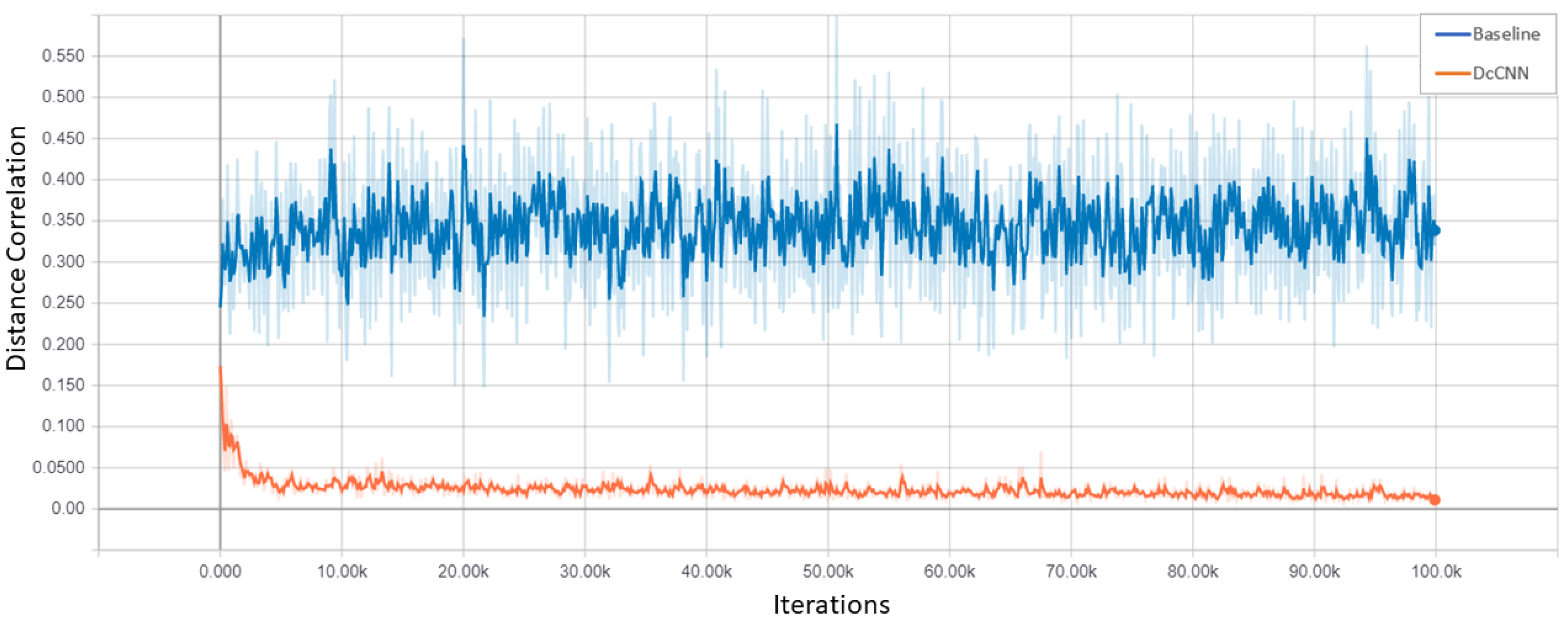
3.1. Distance Correlation

Distance correlation measures not only linear, but also non-linear dependencies between two random variables $B_{1,\dots ,p}$ and $F_{1,\dots ,p}$, unlike the Pearson correlation coefficient [21] which measures only linear dependencies. In our proposed approach, B is the dataset bias variable whereas F is features extracted from ANN and CNN and p is the total number of samples. The distance correlation is the square root of:

$$\begin{array}{c}\hfill {\mathit{DC}}^2(B,F)=\left\{\begin{array}{cc}\frac{v^2(B,F)}{\sqrt{v^2(B,B)v^2(F,F)}}\hfill & \mathrm{if}{v}^2(B,B)v^2(F,F)>0\hfill \\ 0\hfill & \mathrm{else}0\hfill \end{array}\right.\end{array}$$

(1)

where ${DC}^2(B,F)$ varies between 0 and 1 and indicates that variables B and F have dependencies, and $DC(B,F)=0$ only when the variables B and F are independent. $v^2(B,F)$ is the distance covariance between a pair of variables and $v^2(B,B)$, $v^2(F,F)$ is the distance variance as defined in [22]. The distance covariance is normalized by the distance variances.

3.2. Decorrelation in Objective Function

In our study, we use the squared distance correlation as a decorrelation function. This function is minimized to decorrelate features learned by the networks from the biases. This means that we want to find parameters of the network, such as F features, have a minimal distance correlation with the B bias variable. We added the decorrelation function term to the standard objective function. The objective function is given as:

$$J\left(\theta \right)=\underset{\theta }{min}(1-\lambda )L(Y,\widehat{Y})+\lambda {\mathit{DC}}^2(B,F)$$

(2)

The regular loss function (L) in Equation (2) could be binary cross-entropy, softmax loss, or mean-squared error depending on the nature of the tasks. The $\lambda$ in the objective function is a hyperparameter that controls the relative importance of the decorrelation function in relation to the loss function. Y and $\widehat{Y}$ are true and classifier outputs, respectively, whereas B is bias variable and F is features extracted from the model. Optimizing the combination of these two losses not only helps to mitigate bias but also tries to achieve higher classification accuracy. Depending on the size of the dataset and the overfitting issue, one can also add a regularizer L2 loss function in the objective function for weight decay purposes.

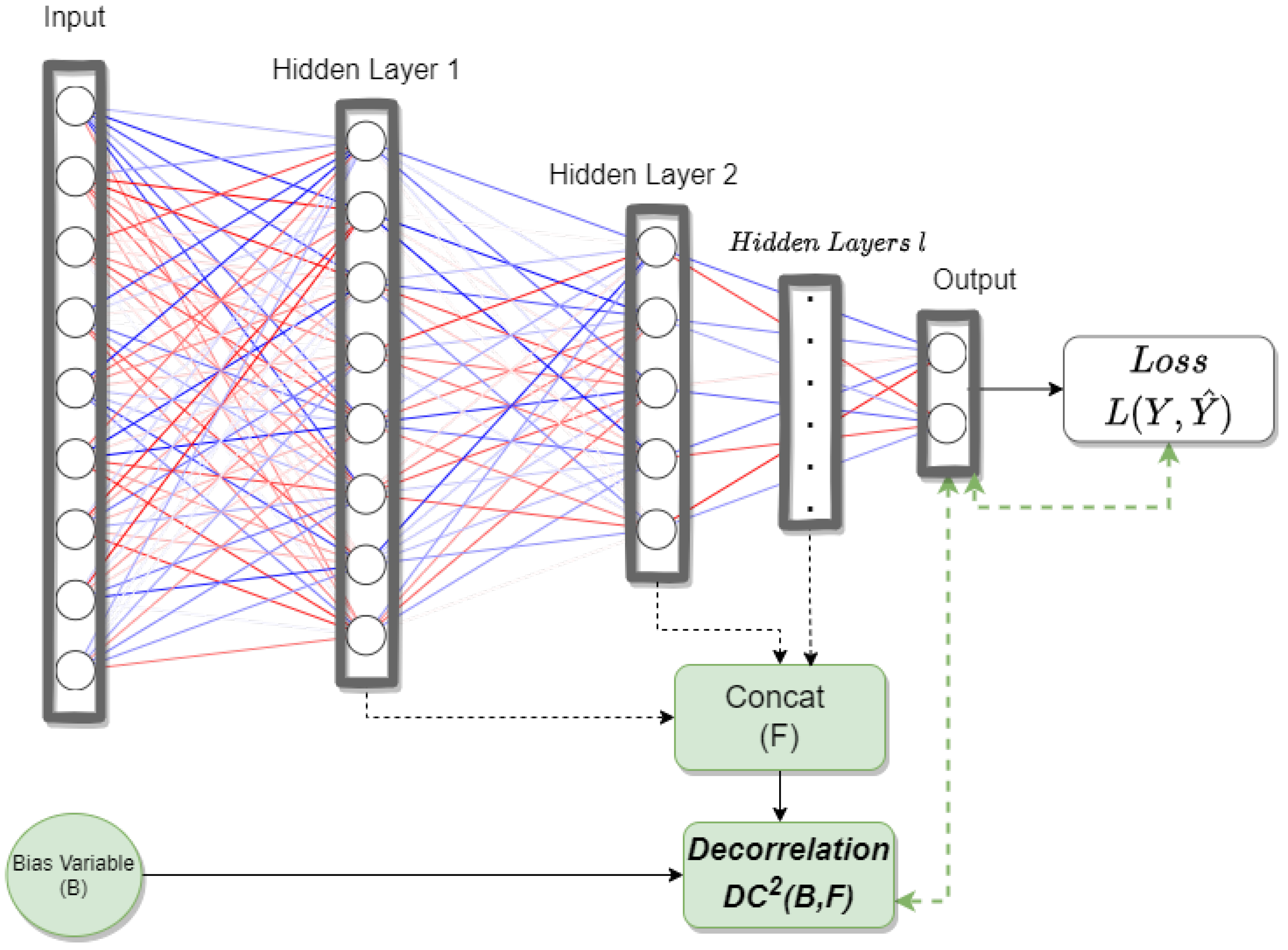
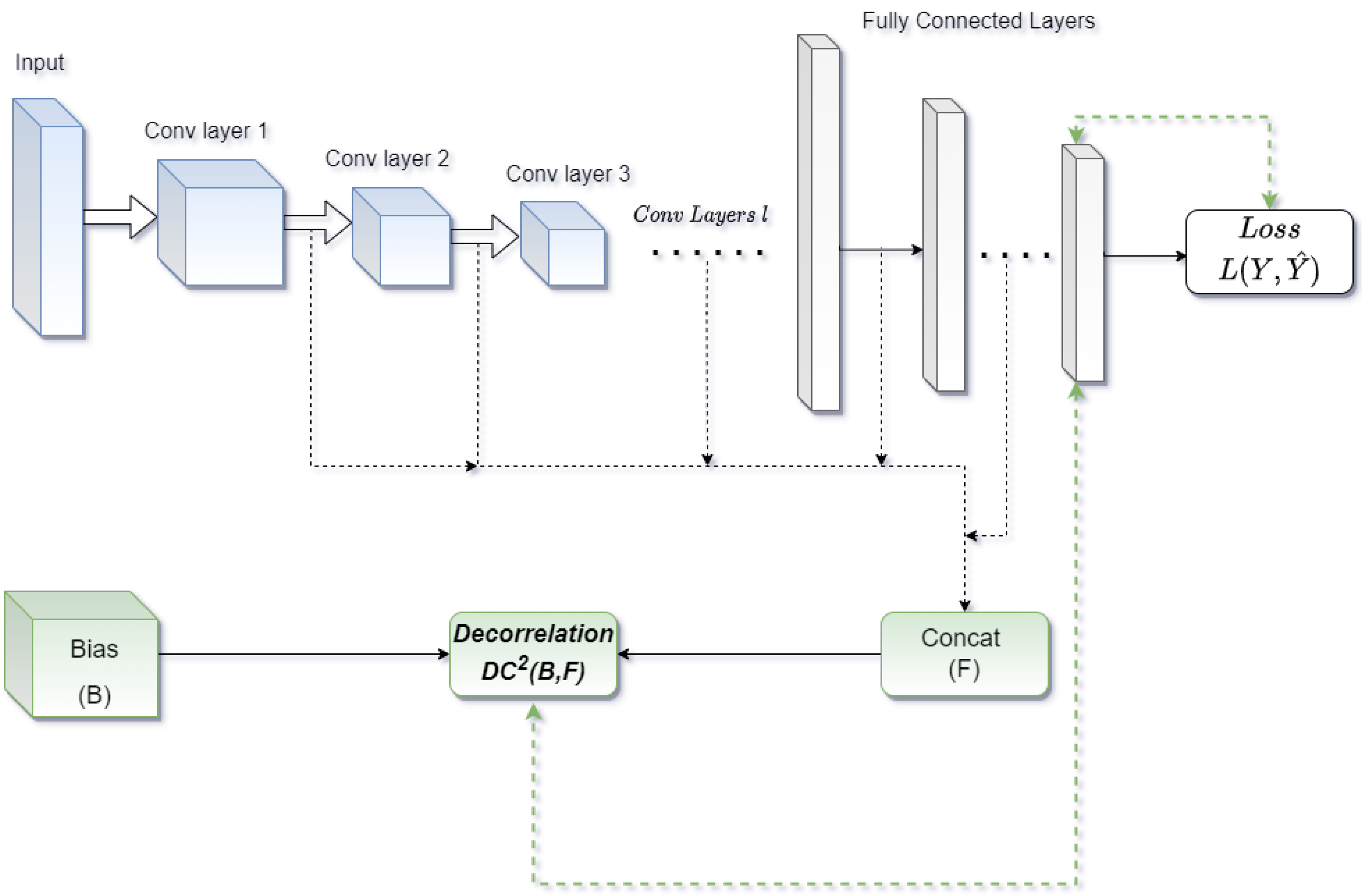
3.3. DcANN and DcCNN

ANNs are suited for modeling complex small datasets. For DcANN, we use the same architecture used in ANN which consists of an input layer, multiple hidden layers $h^{1,\dots ,l}$, and an output layer with only the difference of using hidden layer output values as feature F in decorrelation loss function. The other input to the decorrelation loss function is bias B which can be N-dimensional and include more than one bias type. The framework of our model DcANN is shown in Figure 1. The output of first hidden layer [23] is given by:

$$\begin{array}{cc}\hfill h_j^1=\sum _{j=1}^p{w}_{\mathit{ı}j}^1{\mathrm{x}}_i+b_j^1& \mathrm{where}j=1,\dots ,s\hfill \\ \hfill F=h^{1,\dots ,l}\end{array}$$

(3)

Here, x is the input size of p and after applying a transfer function to $f(h_j^1)$ becomes the output of the first hidden layer, whereas w and b are weights and biases, i.e., $\theta$ parameters of the neural network. The variable (s) denotes the total number of hidden units in the first hidden layer and (l) denotes the total number of layers. We use the output of the first hidden layer $h^1$ as input F to our decorrelation function to reduce the dependencies of these output values on biases. Of course, it may be more appropriate to use just one or combinations of other layer outputs depending on the types of applications.

For DcCNN or DcDNN, we follow the same technique used in ANN. We implemented decorrelation loss function and applied either a CNN or DNN architecture. We propose our DcCNN architecture as in Figure 2. The output of the first convolutional layer [23] is given by:

$$\begin{array}{c}\hfill Z^1=W^1\ast X\\ \hfill F=Z^{1,\dots ,l}\end{array}$$

(4)

In Equation (4), X is the two-dimensional or three-dimensional input size of p. * denotes the convolution operation. We apply a transfer function and max-pooling to $Z^{1,\dots ,l}$ to the output of convolutional layers and concatenate them together to use as features for the decorrelation function. We use the first layer output $Z^1$ as input F to our decorrelation function to reduce the dependencies of these output values on biases. As in the DcANN case, using just one or combinations of other layer outputs as features might be more beneficial depending on the complexity of task.

3.4. Experimental Setup

In order to evaluate our proposed generic method, we explore five different scenarios and different types of biases. To validate our proposed approach, we utilize a simulated biased dataset [7] generated specifically to check the performance of the model in mitigating the bias. Datapoints are generated using four Gaussians whose magnitudes $m_1$ and $m_2$ are controlled by sampling from two different uniform distributions to classify into two groups. We implement three layers of 3 × 3 convolutions followed by tanh activation and max-pooling. This is followed by one hidden layer with 16 dimensions. The output of the last convolutional layer is used as feature F, whereas $m_2$ is a bias variable B since we assume $m_1$ is the main reason for discrimination between two groups. We use a mini-batch size of 256 and the hyperparameter ($\lambda$) of 0.7.

We consider commonly used standard datasets such as the German credit dataset and UCI adult dataset [24] which have been examined for biases. We consider age as a bias variable for the German credit datasets and gender as a bias variable for the UCI Adult dataset as shown in

Table 1. Description of German Credit and Adult Datasets.

Datasets	Bias Variable	Class Labels
German Credit	Age	Good and Bad Credit
UCI Adult	Gender	Income: >50 K and ≤50 K

. The basic three- and two-layer DcANN model is implemented for the adult and German datasets, respectively, and compared with existing mitigation algorithms. For the German dataset, there are two layers with 50 and 10 dimensions with ReLU activations except the last layer with sigmoid activation. We use a mini-btach size of 100 with a dropout of 0.5 and the hyperparameter ($\lambda$) of 0.9. Detailed analysis of $\lambda$ is give in Section 4. The regularization weight decay parameter is set to 0.05. For the adult dataset, we construct three layers with 200, 100, and 50 dimensions. The rest of the configurations used for the adult dataset is the same as for the German dataset except for the mini-batch size of 1024. The output of the last hidden layer is used as feature F, whereas age and gender are used as bias variable B for the German and adult dataset, respectively.

We also use the MNIST image dataset [25] to check the performance of the proposed approach of DcCNN. Since the dataset is grayscale images with no bias and specifically designed for digit classification, we decided to utilize [6] the approach of intentionally planting color bias in the MNIST dataset. A few examples from the color-biased MNIST dataset are shown in Figure 3a. The training dataset consists of colored digits which are randomly sampled from the normal distribution of the corresponding mean and variance. So, the ten colors with their mean color value are assigned to each digit. The variance values such as 0.02, 0.03, 0.035, 0.045, 0.05 are also explored in this experiment. The smaller variance value means more color bias. These variance values controlled the amount of color bias in the training dataset. The testing dataset is unbiased. Colors are assigned randomly to each digit in the testing dataset. For this dataset, we apply the DcCNN method and implemented the same network architecture as in [6], i.e., four convolution layers, followed by average pooling. We use softmax loss and decorrelation loss with $\lambda =0.9$. For decorrrelation loss, we use the output of the first convolutional layer as features F whereas mean RGB color values are used as bias B. RMSprop optimizer with a mini-batch size of 1200 and a learning rate (lr) scheduler with an initial lr of 0.01 with a decay of 0.5 is used.

Another way of adding color bias in the MNIST dataset [26] is dividing the dataset to predict binary labels where 0–4 digits are assigned as labels 0 and 5–9 digits are assigned as label one and then flipping the label with a 25% probability and color with probability value which depends on the training environment. We combine these two training environments in one for our proposed method. According to labels in the training dataset, digit groups (i.e., 0–4 digits group and 5–9 digits group) are assigned red or green colors in a way that is strongly correlated with label 0 and label 1. For the testing dataset, the direction of correlation is changed; for example, if label 0 is red, then in the testing dataset, label 0 is green. We term this as the reversed color-biased MNIST dataset since the relation with bias variable in training and the testing dataset is exactly opposite. Figure 3b shows some of the samples taken from the reversed color-biased MNIST dataset. We apply DcCNN with CNN architecture by using two convolution layers and two fully connected layers. We use the same batch size and optimizer as in the color-biased MNIST dataset. The network is trained with $\lambda =0.99$ and a learning rate (lr) scheduler with an initial lr of 0.001 with a decay of 0.5. In addition to this, an optimizer weight decay of 0.005 is used. Similar to the color-biased MNIST dataset, the output of the first convolutional layer is used to reduce their association with mean RGB color values.

We implemented DcCNNs to all our DcCNNs and DcANNs from scratch in python on the AWS Deep Learning AMIs [27] to accelerate deep learning in the cloud, at any scale using the TensorFlow platform [28] and cuDNN library [29]. An Amazon EC2 P2 Instance is used to train the dataset using deep learning. P2 instances provide eight high-speed GPUs, parallel processing cores, and single and double-precision floating-point performance to speed up the training processes.

4. Results

4.1. Simulated Dataset

To validate the performance of our proposed approach DcCNN, we apply our method and baseline to simulated the dataset to mitigate bias planted in the dataset. The baseline model is trained with $\lambda =0$ where decorrelation is not performed to mitigate the bias $m_2$. Figure 4 shows tSNE plots of learned features for baseline as well as DcCNN models. The color bar indicates the value of bias variable $m_2$. From the plots, we can see that there is a correlation between features and $m_2$ for the baseline model whereas features learned by DcCNN have a roughly uniform distribution of features across all values of $m_2$ indicating no dependency of features on bias $m_2$. This indicates that our proposed DcCNN successfully mitigates the bias present in the dataset.

We also plotted the decorrelation function against iterations in Figure 5 to compare the performance of models in regards to reducing the statistical dependence between features and bias variables. This figure shows the unsmoothed distance correlation values in light blue and light orange colors. In contrast, dark blue and dark orange colors indicate the smoothed distance correlation values which are calculated using exponential moving average. Smoothing is used to observe the overall trend. It shows that the distance correlation between features and bias variable decreases as the number of iterations increases for DcCNN as opposed to the baseline model.

4.2. Age Biased German Dataset

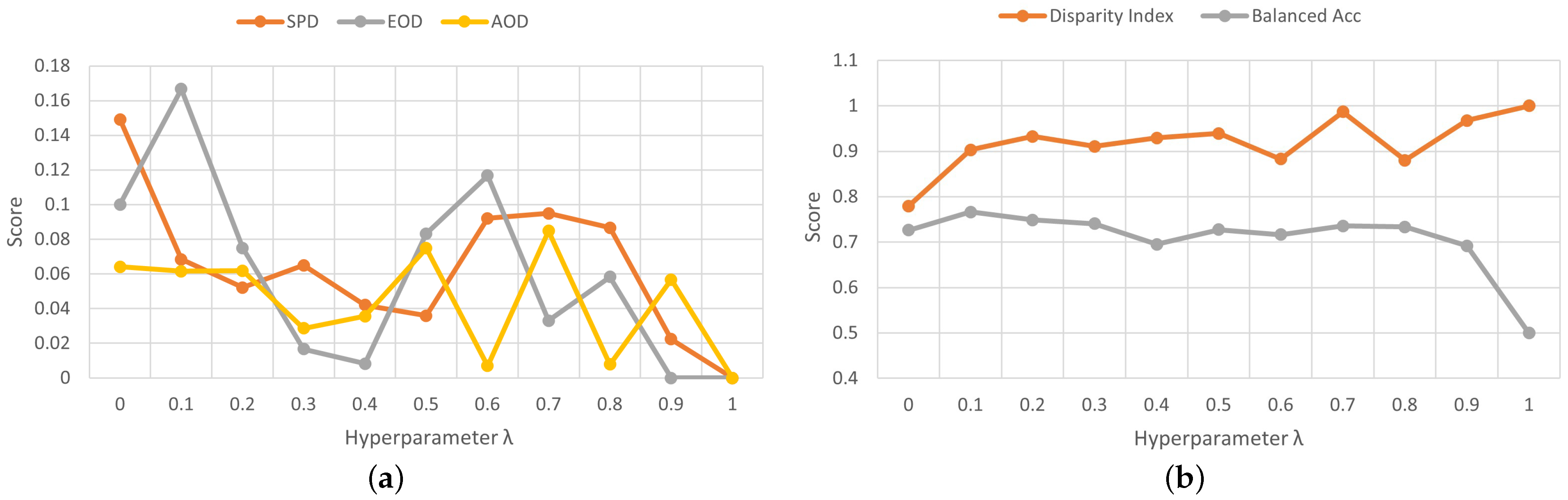
For the age-biased German dataset, we train a model to classify credit score levels and to reduce the gender bias of the baseline model. Furthermore, we analyze the performance of different bias mitigation approaches using fairness metrics.

4.2.1. Hyperparamter $\lambda$ Analysis

The hyperparameter $\lambda >0$ defines the strength or relative importance of the decorrelation function in relation to the loss function, and hence, it plays a crucial role in deciding the importance of the decorrelation task for bias mitigation. The higher value of $\lambda$ means features learned by the network are highly decorrelated with bias which might impact the ability of the network to do certain tasks such as classification. A lower value of $\lambda$ would mean less bias reduction relative to a higher value. The better performance is achieved by trying different values of $\lambda$ depending upon the requirement of applications.

Figure 6 plots fairness scores and accuracies for different values of $\lambda$ for the age-biased German dataset. We can infer from the plot Figure 6a that for the German dataset, SPD, EOD, and AOD values somewhat decrease as the value of $\lambda$ increases. The main reason behind this is the decorrelation between features learned by the model and age bias in the German dataset increases as the value of $\lambda$ increases. In Figure 6b, we observe that DI increases as the value of $\lambda$ increases whereas there is a slight drop in balanced accuracy as the value of $\lambda$ increases. In order to achieve maximum fairness or bias reduction, we select $\lambda$ = 0.9 since the lowest values of SPD and EOD and the highest value of DI are observed for the same. The values for $\lambda$ may vary for different tasks depending upon network architecture and the complexity of the task.

4.2.2. Evaluation Fairness Metrics

In general, to access the performance of the fair model which indicates no discrimination against the bias or protected attribute, we report widely-used fairness metrics for bias mitigation methods. These protected attributes include gender, age, color, race, religion, etc. In this study, we will focus on metrics to evaluate group fairness based on age and gender. The fair model will provide predictions that are not influenced by protected attributes. Four metrics have been selected to evaluate the bias mitigation ability of the proposed approach since testing datasets of age-biased German and gender-biased adult datasets are not unbiased and contain age and gender bias, respectively.

We use the Demographic Parity or Statistical Parity Difference (SPD) fairness metric [30] to check if decisions are independent of protected attributes. Disparate Impact (DI) [31] is the same as SPD but formulated as proportion, respectively. SPD and DI are given as:

$$\begin{array}{c}\hfill \mathrm{SPD}=\mathrm{P}(\widehat{Y}=1|B=0)-\mathrm{P}(\widehat{Y}=1|B=1)\end{array}$$

(5)

$$\begin{array}{c}\hfill \mathrm{DI}=\frac{\mathrm{P}(\widehat{Y}=1|B=1)}{\mathrm{P}(\widehat{Y}=1|B=0)}\end{array}$$

(6)

The Equality of Odds Difference (EOD) metric [32] is used for separation, i.e., to check the independence of the decision and protected attribute separately for individuals. EOD measures the difference in true positive rates for protected and unprotected groups whereas Average Odds Difference (AOD) [32] measures the difference between the true-positive rates as well as false-positive rates for each group. EOD and AOD are formulated as:

$$\begin{array}{c}\hfill \mathrm{EOD}={\mathrm{TPR}}_{B=0}-{\mathrm{TPR}}_{B=1}\end{array}$$

(7)

$$\begin{array}{c}\hfill \mathrm{AOD}=0.5\ast [({\mathrm{FPR}}_{B=0}-{\mathrm{FPR}}_{B=1})+({\mathrm{TPR}}_{B=0}-{\mathrm{TPR}}_{B=1})]\end{array}$$

(8)

In the above Equations (5)–(8), B is bias variable which can be age or gender and is 0 when it represents a privileged group and 1 when it represents an unprivileged group. P is the classification probability whereas $\widehat{Y}$ is model prediction. $\mathrm{FPR}$ and $\mathrm{TPR}$ represent a false positive rate and true positive rate, respectively. Lower values of SPD, EOD, and AOD indicate less bias, and higher values of DI show more fairness and less bias. Balanced accuracy is calculated as the average of sensitivity and specificity.

4.2.3. Comparative Evaluations

We compare the performance of our proposed DcANN with other existing pre-processing methods as shown in

Table 2. Fairness scores and Balanced accuracies of predictions for age-biased German dataset for different methods.

Methods	SPD	EOD	AOD	DI	BA
Baseline	−0.3162	−0.318	−0.2876	0.3112	0.6534
Reweighing	−0.2049	−0.2318	−0.2016	0.6229	0.6687
Optimized pre	−0.0351	0.0254	−0.0639	0.9421	0.6872
Advers-Debias	0.0713	0.0393	0.0931	1.0834	0.6633
B-DcANN ($\lambda$ = 0)	−0.1491	−0.1	−0.0642	0.7798	0.7262
DcANN	−0.03144	−0.03918	0.06223	0.95927	0.7093

on a holdout testing dataset. We report all fairness metrics and balanced accuracies for all the methods. The existing methods such as the baseline model, reweighing, optimized pre-processing, and adversarial debiasing are implemented using the AIF360 [33] open source Python toolkit. The baseline model is simple the ANN model where unprocessed data are used and bias mitigation method is not applied. Baseline DcANN (B-DcANN) has the same architecture as DcANN but with $\lambda =0$ which means decorrelation is not present for bias mitigation. The main difference between the baseline model and B-DcANN is that B-DcANN uses regularization parameters such as dropout and weight decay. We notice that regularization helps the model in achieving higher accuracy as can be seen in Table 2.

As we can see, our proposed method DcANN significantly reduces SPD, EOD, and AOD as compared to other methods without compromising the accuracy. The DI is higher for our DcANN method compared to other methods except for adversarial debiasing. However, as we can see from other fairness metrics and especially accuracy, adversarial debiasing does not provide a significant reduction in bias without significantly comprising accuracy when compared to our DcANN method. In general, we can say that our model performs best on all fairness metrics.

4.3. Gender-Biased Adult Dataset

The UCI adult dataset is used to classify income levels and we consider gender as bias. We use the same evaluation metrics as defined in Section 4.2.2 and compare with the same existing mitigation methods mentioned in Section 4.2.3 on a holdout testing dataset for the gender-biased adult dataset. We also compare the performance of our model with the method of fusion introduced in [34]. Authors used the fusion of different combinations of existing bias mitigation methods such as Disparate Impact Remover (DIR) [31], Adversarial Debiasing (Advers-Debias) [13], and Calibrated Equalized Odds (CEO) [35] to provide end-to-end bias mitigation. We use their best method for the comparison.

The results for each method are displayed in

Table 3. Fairness scores and balanced accuracies of predictions for gender-biased adult dataset for different models.

Methods	SPD	EOD	AOD	DI	BA
Baseline	−0.3752	−0.3716	−0.3258	0.2876	0.7472
Reweighing	−0.2924	−0.3815	−0.3234	0.3831	0.7110
Optimized pre	−0.2144	−0.1991	−0.1945	0.568	0.7231
Advers-Debias	−0.0876	−0.0592	−0.0373	0.5775	0.6656
DIR + Advers-Debias + CEO	−0.0301	0.0785	0.051	-	0.8113
B-DcANN ($\lambda$ = 0)	−0.3394	−0.1545	−0.1965	0.3025	0.8226
DcANN	−0.0964	0.0657	0.0325	0.8063	0.7747

. The results show that the DcANN model achieves the lowest EOD and AOD and highest DI amongst all methods while the balanced accuracy slightly decreases. The SPD and EOD scores of Adversarial Debiasing are almost similar to the DcANN method. However, as it is seen in the German dataset case, Adversarial Debiasing helps to reduce bias but at the cost of a significant reduction in the accuracy. The fusion model (IR + Advers-Debias + CEO) has the lowest SPD and highest accuracy but it does not perform well on other fairness metrics. Thus, the results suggest that DcANN reduces bias fairly by achieving good results on almost all fairness metrics without significantly compromising balanced accuracy.

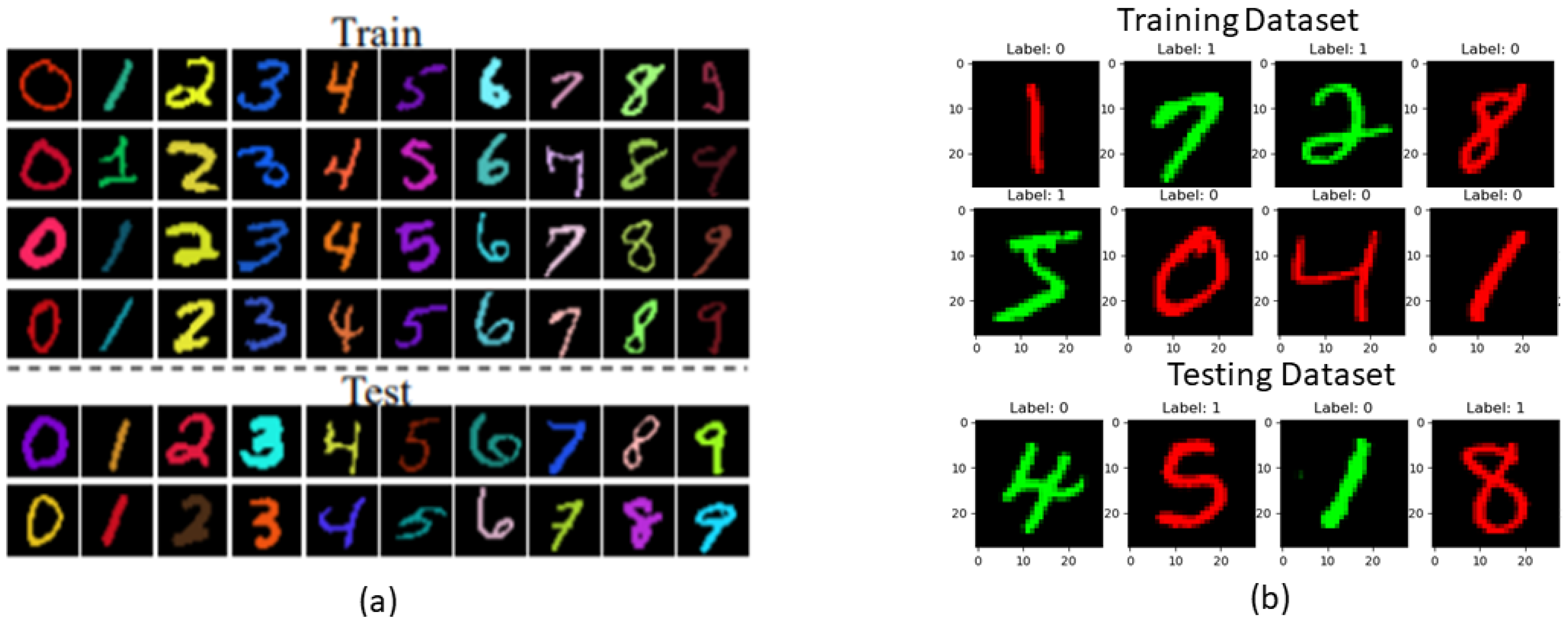
4.4. Color-Biased MNIST Dataset

The color introduced in the dataset misled the model while performing the digit classification task. The model learns the color features instead of learning digit features to categorize the digits. We use the DcCNN model to remove color bias from features learned by the network. The performance of the DcCNN model is compared with existing methods such as Adversarial Training [6] and the Blind Eye method [19]. Adversarial Training without Pre-trained model (Advers Training-no Pretrain) is the same as the Adversarial Training model but it is trained from scratch without using any pre-trained parameters. The baseline model is trained with no decorrelation function, i.e., $\lambda =0$ which means bias mitigation is not performed. The results are included in the

Table 4. Comparison of accuracies for color-biased MNIST dataset for different values of variances among existing methods. Results are calculated on the testing dataset.

Methods	Var = 0.02	Var = 0.03	Var = 0.035	Var = 0.045	Var = 0.05
Baseline	0.4055	0.5996	0.6626	0.7973	0.845
BlindEye	0.6741	0.7883	0.8203	0.8927	0.9159
Advers Training	0.8185	0.9137	0.9306	0.9555	0.9618
Advers Training-no Pretrain	0.7336	0.8516	0.8781	0.9277	0.9429
DcCNN	0.8100	0.8910	0.9250	0.9500	0.9604

and the variance values (Var) control the amount of color bias in the dataset.

The results show that our model DcCNN achieves almost the same accuracies as adversarial training and is better than all other methods for all values of variances. However, in order to achieve the same results using the Adversarial Training method, we need to use pre-trained parameters. If we don’t utilize a pre-trained model and train the model from scratch, then there is a lot of fluctuation in the accuracies. In fact, as shown in Table 4, accuracies dropped by a significant amount for low variance values for Adversarial Training without using the pre-trained model. This indicates that the Adversarial training algorithm is very unstable, and it also requires a lot of fine-tuning. Thus, the DcCNN model is simple and requires less fine-tuning since it has only one hyperparameter ($\lambda$) for fine-tuning to successfully mitigate the color bias while achieving high performance.

4.5. Reversed Color-Biased MNIST Dataset

To analyze the reversed effect of bias and the proposed approach, we use the reversed color-biased MNIST dataset where the bias present in the testing dataset is exactly the opposite of the bias present in the training dataset. This is to validate how well the proposed approach generalizes to the unseen test dataset. In the paper [26], Arjovsky et.al. used an Invariant Risk Minimization (IRM) causal-invariant based approach in multiple training environments to promote out-of-distribution (OOD) generalization by assuming the different environments share the same underlying structural equation model. An ANN classifier is implemented to achieve the same. However, for comparison purposes, we use the same CNN architecture as mentioned in Section 3.4 for all existing methods. Empirical Risk Minimization (ERM) combines the data from all the training environments and uses all features which is similar to the baseline model principle.

The

Table 5. Comparison of accuracies for reversed color-biased MNIST dataset among different methods. Results are calculated on testing dataset.

Methods	Accuracy
Baseline: ERM	0.1115
IRM	0.6208
DcCNN	0.6630

presents the comparison where the ERM method classifies digits based on color bias and hence the lowest accuracy whereas IRM and DcCNN remove the color bias information from the features and classify based on features relevant to digits. The results show that DcCNN achieved an accuracy of 66.30% which is the best across all methods and can successfully mitigate the color bias by learning more digit-relevant features.

5. Discussion

One of the crucial aspects of our proposed method is to mitigate bias without compromising the performance of the model by optimizing the decorrelation loss along with loss related to the task and tuning hyperparameter ($\lambda$). The choice of $\lambda$ depends on the complexity of the task and network architecture. The results from all five datasets outperformed the traditional approaches in mitigating different types of biases. This higher performance indicates that the DcCNN and DcANN models significantly mitigate the bias and present relevant feature information to the network compared to other methods. Further, this also demonstrates the generalization ability of the proposed approach across different domains for bias mitigation.

In Figure 5, we observe the oscillations in distance correlation values. From our experiments, we verify that these oscillations are due to the size of mini-batches. Increasing the batch size not only reduces the oscillations but also leads to an unbiased estimate of distance correlation. We also notice that regularization such as dropout and weight decay helps the baseline model to improve its performance. As for our proposed approach, the input bias variable also plays a vital role and it should clearly define the bias present in the data or task. For example, a possible concern is our proposed method might not show significant improvement for the domain adaptation tasks due to the lack of enough quantitative information about different domains and a limited number of domains. We apply our method for digit domain adaptation tasks [36] where we use MNIST, USPS, SVHN, and synthetic numbers datasets as training and validation datasets. We evaluated the results on the MNIST-M dataset as a test dataset. However, we observed that the improvement using our approach is not that significant. For such cases, we simply recommend collecting and using more domain-relevant information as a bias variable or using domain distributions as a bias variable.

6. Conclusions

The performance of deep learning mainly depends on the quality of data. Failure to account for the quality of data, e.g., biased data in deep learning can lead to erroneous decisions. We propose a new method based on the core idea of reducing the association between features learned by the ANN or CNN models and bias. Additionally, we evaluated proposed models, which we name the DcANN and DcCNN, on five different datasets with different biases such as age, gender, and color. The experimental results demonstrate that features learned by our models are statistically independent of biases or confounds present in the dataset. Our proposed method leverages the ability of the distance correlation function in decorrelation features from data bias without significantly impacting the performance of a network. Furthermore, we observe that our method also performs better than previous approaches to mitigate the bias. Our models are easy, simple, and require fewer hyperparameters to optimize compared to adversarial training. Thus, our models DcCNN and DcANN, despite having numerous methods to achieve bias mitigation, is a promising and effective novel method. Future work will investigate the use of DcDNN in the medical domain to mitigate bias or confounding effects or any irrelevant dependency issues. In addition, we plan to further evaluate the expansion of the proposed method by applying it to pre-trained models and to different types of data variations. Although we did not observe significant change in training times for all our proposed models in comparison with baseline models, we intend to perform a time complexity analysis in the future by measuring the whole training process in terms of training time as the number of dimensions, the complexity of tasks, and the number of layers increases.

References

1. Mehrabi, N.; Morstatter, F.; Saxena, N.; Lerman, K.; Galstyan, A. A survey on bias and fairness in machine learning. ACM Comput. Surv. (CSUR) 2021, 54, 1–35. [Google Scholar] [CrossRef]
2. Kärkkäinen, K.; Joo, J. Fairface: Face attribute dataset for balanced race, gender, and age. arXiv 2019, arXiv:1908.04913. [Google Scholar]
3. Tommasi, T.; Patricia, N.; Caputo, B.; Tuytelaars, T. A deeper look at dataset bias. In Domain Adaptation in Computer Vision Applications; Springer: Berlin/Heidelberg, Germany, 2017; pp. 37–55. [Google Scholar]
4. LeCun, Y.; Boser, B.; Denker, J.; Henderson, D.; Howard, R.; Hubbard, W.; Jackel, L. Handwritten digit recognition with a back-propagation network. In Proceedings of the Advances in Neural Information Processing Systems, Denver, CO, USA, 27–30 November 1989; Volume 2. [Google Scholar]
5. Kamiran, F.; Calders, T. Data preprocessing techniques for classification without discrimination. Knowl. Inf. Syst. 2012, 33, 1–33. [Google Scholar] [CrossRef] [Green Version]
6. Kim, B.; Kim, H.; Kim, K.; Kim, S.; Kim, J. Learning not to learn: Training deep neural networks with biased data. In Proceedings of the IEEE/CVF Conference on Computer Vision and Pattern Recognition, Long Beach, CA, USA, 15–20 June 2019; pp. 9012–9020. [Google Scholar]
7. Adeli, E.; Zhao, Q.; Pfefferbaum, A.; Sullivan, E.V.; Fei-Fei, L.; Niebles, J.C.; Pohl, K.M. Representation learning with statistical independence to mitigate bias. In Proceedings of the IEEE/CVF Winter Conference on Applications of Computer Vision, Waikoloa, HI, USA, 3–8 January 2021; pp. 2513–2523. [Google Scholar]
8. Hagan, M.T.; Demuth, H.B.; Beale, M. Neural Network Design; PWS Publishing Co.: Stillwater, OK, USA, 1997. [Google Scholar]
9. Kasieczka, G.; Shih, D. DisCo Fever: Robust Networks through Distance Correlation. arXiv 2020, arXiv:2001.05310. [Google Scholar]
10. Calmon, F.; Wei, D.; Vinzamuri, B.; Natesan Ramamurthy, K.; Varshney, K.R. Optimized pre-processing for discrimination prevention. In Proceedings of the Advances in Neural Information Processing Systems, Long Beach, CA, USA, 4–9 December 2017; Volume 30. [Google Scholar]
11. Li, Y.; Vasconcelos, N. Repair: Removing representation bias by dataset resampling. In Proceedings of the IEEE/CVF Conference on Computer Vision and Pattern Recognition, Long Beach, CA, USA, 15–20 June 2019; pp. 9572–9581. [Google Scholar]
12. Dinsdale, N.K.; Jenkinson, M.; Namburete, A.I. Deep learning-based unlearning of dataset bias for MRI harmonisation and confound removal. NeuroImage 2021, 228, 117689. [Google Scholar] [CrossRef] [PubMed]
13. Zhang, B.H.; Lemoine, B.; Mitchell, M. Mitigating unwanted biases with adversarial learning. In Proceedings of the 2018 AAAI/ACM Conference on AI, Ethics, and Society, New Orleans, LA, USA, 2–3 February 2018; pp. 335–340. [Google Scholar]
14. Mandis, I.S. Reducing Racial and Gender Bias in Machine Learning and Natural Language Processing Tasks Using a GAN Approach. Available online: https://terra-docs.s3.us-east-2.amazonaws.com/IJHSR/Articles/volume3-issue6/2021_36_p17_Mandis.pdf (accessed on 15 November 2021).
15. Goodfellow, I.; Pouget-Abadie, J.; Mirza, M.; Xu, B.; Warde-Farley, D.; Ozair, S.; Courville, A.; Bengio, Y. Generative adversarial nets. In Proceedings of the Advances in Neural Information Processing Systems, Montreal, QC, Canada, 8–13 December 2014; Volume 27. [Google Scholar]
16. Sadeghi, B.; Yu, R.; Boddeti, V. On the global optima of kernelized adversarial representation learning. In Proceedings of the IEEE/CVF International Conference on Computer Vision, Seoul, Korea, 27 October–2 November 2019; pp. 7971–7979. [Google Scholar]
17. Zhao, T.; Dai, E.; Shu, K.; Wang, S. Towards Fair Classifiers without Sensitive Attributes: Exploring Biases in Related Features. 2022. Available online: http://www.cs.iit.edu/~kshu/files/fair-wsdm22.pdf (accessed on 20 January 2022).
18. Wang, T.; Zhao, J.; Yatskar, M.; Chang, K.W.; Ordonez, V. Balanced datasets are not enough: Estimating and mitigating gender bias in deep image representations. In Proceedings of the IEEE/CVF International Conference on Computer Vision, Seoul, Korea, 27 October–2 November 2019; pp. 5310–5319. [Google Scholar]
19. Alvi, M.; Zisserman, A.; Nellåker, C. Turning a blind eye: Explicit removal of biases and variation from deep neural network embeddings. In Proceedings of the European Conference on Computer Vision (ECCV) Workshops, Munich, Germany, 8–14 September 2018. [Google Scholar]
20. Wang, R.; Karimi, A.H.; Ghodsi, A. Distance correlation autoencoder. In Proceedings of the IEEE 2018 International Joint Conference on Neural Networks (IJCNN), Rio de Janeiro, Brazil, 8–13 July 2018; pp. 1–8. [Google Scholar]
21. Lee Rodgers, J.; Nicewander, W.A. Thirteen ways to look at the correlation coefficient. Am. Stat. 1988, 42, 59–66. [Google Scholar] [CrossRef]
22. Székely, G.J.; Rizzo, M.L.; Bakirov, N.K. Measuring and testing dependence by correlation of distances. Ann. Stat. 2007, 35, 2769–2794. [Google Scholar] [CrossRef]
23. Patil, P. Flexible Image Recognition Software Toolbox (First); Oklahoma State University: Stillwater, OK, USA, 2013. [Google Scholar]
24. Dua, D.; Graff, C. UCI Machine Learning Repository. (University of California, Irvine, School of Information, 2017). Available online: http://archive.ics.uci.edu/ml (accessed on 1 August 2020).
25. LeCun, Y.; Cortes, C. MNIST Handwritten Digit Database. 2010. Available online: http://yann.lecun.com/exdb/mnist/ (accessed on 25 July 2020).
26. Arjovsky, M.; Bottou, L.; Gulrajani, I.; Lopez-Paz, D. Invariant risk minimization. arXiv 2019, arXiv:1907.02893. [Google Scholar]
27. Deep Learning Ami—Developer Guide. AWS Deep Learning AMIs Documentation. Available online: https://docs.aws.amazon.com/dlami/latest/devguide/dlami-dg.pdf (accessed on 12 February 2019).
28. Abadi, M.; Agarwal, A.; Barham, P.; Brevdo, E.; Chen, Z.; Citro, C.; Corrado, G.; Davis, A.; Dean, J.; Devin, M.; et al. TensorFlow: Large-Scale Machine Learning on Heterogeneous Systems. 2015. Available online: https://www.tensorflow.org/ (accessed on 6 January 2019).
29. Chetlur, S.; Woolley, C.; Vandermersch, P.; Cohen, J.; Tran, J.; Catanzaro, B.; Shelhamer, E. Cudnn: Efficient primitives for deep learning. arXiv 2014, arXiv:1410.0759. [Google Scholar]
30. Kusner, M.J.; Loftus, J.; Russell, C.; Silva, R. Counterfactual fairness. In Proceedings of the Advances in Neural Information Processing Systems, Long Beach, CA, USA, 4–9 December 2017; Volume 30. [Google Scholar]
31. Feldman, M.; Friedler, S.A.; Moeller, J.; Scheidegger, C.; Venkatasubramanian, S. Certifying and removing disparate impact. In Proceedings of the 21th ACM SIGKDD International Conference on Knowledge Discovery and Data Mining, Sydney, Australia, 10–13 August 2015; pp. 259–268. [Google Scholar]
32. Li, X.; Cui, Z.; Wu, Y.; Gu, L.; Harada, T. Estimating and improving fairness with adversarial learning. arXiv 2021, arXiv:2103.04243. [Google Scholar]
33. Bellamy, R.K.; Dey, K.; Hind, M.; Hoffman, S.C.; Houde, S.; Kannan, K.; Lohia, P.; Martino, J.; Mehta, S.; Mojsilovic, A.; et al. AI Fairness 360: An extensible toolkit for detecting, understanding, and mitigating unwanted algorithmic bias. arXiv 2018, arXiv:1810.01943. [Google Scholar]
34. Feldman, T.; Peake, A. End-To-End Bias Mitigation: Removing Gender Bias in Deep Learning. arXiv 2021, arXiv:2104.02532. [Google Scholar]
35. Pleiss, G.; Raghavan, M.; Wu, F.; Kleinberg, J.; Weinberger, K.Q. On fairness and calibration. In Proceedings of the Advances in Neural Information Processing Systems, Long Beach, CA, USA, 4–9 December 2017; Volume 30. [Google Scholar]
36. Ganin, Y.; Ustinova, E.; Ajakan, H.; Germain, P.; Larochelle, H.; Laviolette, F.; Marchand, M.; Lempitsky, V. Domain-adversarial training of neural networks. J. Mach. Learn. Res. 2016, 17, 2096–2030. [Google Scholar]
Figure 1. Proposed DcANN architecture: Black dashed lines denote the output of hidden layers l which are combined together to represent learned features. Green dashed lines indicate the start of the learning process where backward arrows show back-propagation using their respective gradient values while forward arrows show forward paths with updated parameters. Network parameters are updated as per the objective function.
Futureinternet 14 00110 g001
Figure 2. Proposed DcDNN architecture. Black dashed lines denote the output of convolutional layers l which are combined together to represent learned features. Green dashed lines indicate the start of the learning process where backward arrows show back-propagation using their respective gradient values while forward arrows show forward paths with updated parameters. Network parameters are updated as per the objective function.
Futureinternet 14 00110 g002
Figure 3. Colored MNIST Training and Testing Datasets Examples with color bias: (a) Some image examples of color-biased MNIST dataset - Modified MNIST dataset with a color bias for each digit. Taken from [6] (b) Some image examples of reversed color-biased MNIST dataset—Binary group based color bias prepared for IRM [26].
Futureinternet 14 00110 g003
Figure 4. tSNE plots of learned features for different methods: (a) For Baseline CNN model [7] (b) For DcCNN model.
Futureinternet 14 00110 g004
Figure 5. Distance correlation between learned features and bias m 2 for the simulated dataset.
Futureinternet 14 00110 g005
Figure 6. Fairness scores and accuracies for different values of λ : (a) SPD, EOD and AOD scores Vs λ (b) DI scores and Accuracies Vs λ .
Futureinternet 14 00110 g006