Anomalous Vehicle Recognition in Smart Urban Traffic Monitoring as an Edge Service ^†

Abstract

The past decades witnessed an unprecedented urbanization and the proliferation of modern information and communication technologies (ICT), which makes the concept of Smart City feasible. Among various intelligent components, smart urban transportation monitoring is an essential part of smoothly operational smart cities. Although there is fast development of Smart Cities and the growth of Internet of Things (IoT), real-time anomalous behavior detection in Intelligent Transportation Systems (ITS) is still challenging. Because of multiple advanced features including flexibility, safety, and ease of manipulation, quadcopter drones have been widely adopted in many areas, from service improvement to urban surveillance, and data collection for scientific research. In this paper, a Smart Urban traffic Monitoring (SurMon) scheme is proposed employing drones following an edge computing paradigm. A dynamic video stream processing scheme is proposed to meet the requirements of real-time information processing and decision-making at the edge. Specifically, we propose to identify anomalous vehicle behaviors in real time by creatively applying the multidimensional Singular Spectrum Analysis (mSSA) technique in space to detect the different vehicle behaviors on roads. Multiple features of vehicle behaviors are fed into channels of the mSSA procedure. Instead of trying to create and define a database of normal activity patterns of vehicles on the road, the anomaly detection is reformatted as an outlier identifying problem. Then, a cascaded Capsules Network is designed to predict whether the behavior is a violation. An extensive experimental study has been conducted and the results have validated the feasibility and effectiveness of the SurMon scheme.

1. Introduction

The past decades have been witnessing a global-wise urbanization at an unprecedented speed. According to the World Urbanization Prospects by the United Nations Department of Economic and Social Affairs (UN DESA) Population Division, by 2014, 54% of the population (3.9 billion) in the world lived in urban areas, and this percentage is visioned to achieve 66% by 2050 [1]. While a larger population, more attractive services, and advanced infrastructures bring prosperity, urbanization also incurs many new challenges to city administrators and urban planners. It is non-trivial to provide a satisfactory living quality and maintain the sustainability of smart cities. Real-time information collection and decision-making are essential for a good understanding of dynamic city elements and timely reactions to emergencies [2,3]. Pervasively deployed smart sensors and devices led us into the era of Internet of Things (IoT), which provides a solid foundation for instant decision-making [4]. Situational awareness (SAW) is among the most crucial issues in smart cities [5,6]. In terms of safety, security, and sustainability of smart cities, urban surveillance services, such as object-of-interest identification [7] and anomalous behavior recognition [8], require not only high accuracy performance, but also real-time data-driven decision-making to avoid unacceptable consequences resulting from insufficient data assessment or incorrect event prediction [3]. However, it is a very challenging task to process an overwhelmingly large amount of urban surveillance data in a timely manner, which is dynamic, heterogeneous, and very diverse.

Among the top concerned topics in smart cities, urban traffic surveillance is an indispensable component. Road safety is an important target in the global Sustainable Development Goals (SDGs). By 2030, the goal is to provide a safe, affordable, accessible and sustainable transport system for all residents [9]. Abnormal driving behaviors have been a challenge for decades since it often seriously jeopardizes the efficiency of traffic, endangers road safety, and even results in public emergencies. Therefore, it is critical to detect and interpret abnormal driving behaviors as early as possible. With the proliferation and ubiquitous deployment of IoTs, traditional solutions like human monitoring on site are being converted into many more automatic and intelligent ways. On the one hand, traffic data can be collected in real time and transferred to cloud centers where machine learning (ML) algorithms will be applied to recognize abnormal traffic patterns. On the other hand, nowadays, with ubiquitously presented smart devices, edge computing [10] rises as a new distributed computing paradigm at the network edge allowing onsite artificial intelligence much closer to the source data for real time decision-making [11,12,13]. Being considered as an extension of cloud computing, edge computing has shown many advantages and is promising to meet the requirements from smart city surveillance applications [14]. Using ubiquitously deployed computing, communication and storage at the edge, edge computing provides on-site/near-site storage and real-time task-processing capabilities, particularly for latency-sensitive applications [15].

Currently, regarding edge computing, there is a close concept named fog computing. For the sake of clarity in this paper, though fog computing emphasizes more on fog servers (like cloudlets or powerful laptops), while edge computing is closer to the network edge where computing nodes could be sensors or actuators; these two concepts will be treated the same, and the term edge computing will be used mostly in the rest of this paper.

Because of the superior performance, Deep Neural Networks (DNNs) are widely adopted in pattern recognition applications [16]. To accommodate edge computing, there are many research efforts attempting to deconstruct DNNs and partitioned networks are allocated on different layers through an edge-fog-cloud computational architecture [17]. To accelerate the performance on the resource constrained edge, there are vertical and horizontal collaborations between edge and cloud. With horizontal collaboration, a single DNN layer is divided into partitioned slices that are assigned to a number of edge devices [18]. In this way, the inference parallelism of edge layers is increased to deal with a large amount of urban data. For solutions with a vertical strategy, edge/fog layers only perform simple references and, if a DNN is confident enough to predict with lower level features, there are early exit points [19]. Inference tasks are offloaded to the cloud layer for a more accurate process. While these research efforts have achieved remarkable performance, they have limitations. First, although DNN has an outstanding prediction power, it always requires a large amount of data for training and the max pooling operations will potentially discard substantial information. In addition, DNNs do not consider spatial and orientation information of features since outputs of activation functions are scalars, which could result in failing to predict vehicle behaviors since they are essentially spatio-temporal data. Secondly, all urban data need to be transferred to edge/fog layers or the cloud layer for inference. This could explode network traffic, and, even in extreme situations, there could be no connection at all.

Capsules Network [20] is a recently proposed new class of DNNs. It utilizes capsules instead of artificial neurons for prediction. As a result, instead of scalars after activation between different layers in conventional DNNs, the Capsules Network outputs vectors and the vector directions represent orientations or poses of features, and the length represents the probability of existence. By leveraging dynamic routing by agreement, lower level features only flow into higher level features when they agree with each other. Therefore, the spatial relationship between lower and higher level features is captured. In this regard, the Capsules Network requires less training data, and it intuitively becomes beneficial for applications with spatial-temporal data [21]. The Capsules Network has been proven to achieve better prediction accuracy on the MNIST data set (Modified National Institute of Standards and Technology database). When facing overlapping digits in images, it outperforms other conventional DNNs. There are also studies applying a Capsules Network on spatial-temporal data like vehicle trajectories and urban traffic data; however, the structure is relatively simple and usually there are only two Capsule layers.

In this paper, a Smart Urban traffic Monitoring (SurMon) scheme is proposed following an edge computing paradigm. SurMon explores an online abnormal vehicle detection using multidimensional singular spectrum analysis (mSSA) at the edge. We format this issue as a change point detection problem where the differences of various characteristics of a vehicle behavior will be identified [22]. Following the detection of misbehaved vehicles, a cascaded Capsules Network is adopted to interpret those behaviors to facilitate decision-making to tell whether this behavior is actually abnormal. There are two major components in our cascaded Capsules Network. The first is to take the data of vehicles with suspicious behaviors and recognize whether the behaviors fall into a pre-trained normal pattern. All vehicle data will go into the first Capsules Net. Then, the outputs will be the input of the second Capsules Net with a new routing agreement to decide if this behavior will be agreed by other vehicles. This strategy is based on a common observation: most of the vehicles on roads are non-aggressively of normal behaviors and aggressive behavior patterns are not agreed on by other vehicles. We implemented and tested the SurMon scheme with a public traffic data set from Next Generation Simulation (NGSIM) [23].

This paper is an extension based on one of our earlier conference publications [22], which was inspired by the excellent performance of the SSA algorithms in change point detection in time series [24]. The mSSA algorithm is creatively adopted to catch the differences in the dimension of characteristics of vehicles on the road by reformatting the abnormal vehicle detection problem as a change point detection problem. Instead of depending on pre-defined abnormal behavior patterns, we catch different/suspicious behaviors and then recognize this behavior. The mSSA approach reduces the amount of data to be transmitted to either a fog or a cloud layer. On top of [22], the major contributions of this paper are:

• A novel framework is proposed to detect and recognize abnormal vehicle behaviors by leveraging the mSSA algorithm and Capsules Networks at the edge;
• A new cascaded Capsules Network structure is introduced with a new routing agreement for abnormal vehicle behavior recognition; and
• Extensive experimental studies have been conducted with real-world traffic data that validated the effectiveness of SurMon scheme.

The rest of this paper is organized as follows: Section 2 briefly presents the related work. An overall introduction of the SurMon architecture is given in Section 3. The anomalous vehicle behavior detection procedure using mSSA is discussed in Section 4 and the behavior interpretation scheme using the cascaded Capsules Network architecture is presented in Section 5. Experimental results are reported in Section 6, and Section 7 concludes this paper with some discussions and the future work.

2. Related Work

2.1. Anomaly Vehicle Behavior Detection

A plethora of research efforts are reported in this area [25,26,27], and recently analysis and prediction of behaviors of autonomous driving have attracted more attention [28,29,30]. In this subsection, we provide a concise discussion on works that are closely related to our proposal. A novel deep-learning-based model is proposed for abnormal driving detection [31], in which a stacked sparse autoencoder model is adopted to learn generic driving behavior features from an unlabelled dataset in an unsupervised manner. Then, an error propagation algorithm is used with labeled data to fine-tune the model for a better performance. Corresponding to the behaviors under consideration, there are four patterns defined in this work: normal, drunk/fatigue, reckless, and phone use [31].

A vehicle-edge–cloud framework is suggested to evaluate driving behaviors with deep learning [32], where driving behaviors are marked in three rankings with scores in a descending order: A, B, and C. In this framework, real-time vehicle driving data are transmitted to edge layers for reference, and the cloud exists to train or upgrade the predictive model. Similarly, in another work, researchers leverage edge layers to pre-process traffic video data to reduce network traffic [33]. The processed data will be transmitted to the cloud for vehicle detection and anomaly behavior detection. In contrast, Jiang et al. aim to detect drivers inattention driving behaviors with large scale vehicle trajectory data [34]. In addition, based on the output derived from the inattention detection combining with point of interest and climate data, a Long Short Term Memory (LSTM) based model is deployed to predict driver’s upcoming abnormal operations on the road [34].

Although these reported efforts have achieved remarkable performance in abnormal driving behaviors detection, the application scenarios are different with ours. First, in some research works, the edge layer serves as more like a transponder which receives data from end devices and pre-processes it for preliminary learning or simple features extraction and transmits them to a cloud layer for a complicated reference. Secondly, to recognize abnormal behaviors, prior knowledge is required to pre-define what is an abnormal driving behavior. Therefore, on the one hand, these approaches necessitate large-scale, good quality data sets that cover a sufficient amount of scenarios; on the other hand, in real-world traffic scenarios, the reliability could be weak since, in some cases, normal and abnormal behaviors can exchange.

In this paper, instead of trying to define a complete set of abnormal patterns, our approach trains models with normal patterns that are the most common cases in real-world. Additionally, mSSA is firstly utilized to identify vehicles that behave differently with others, and then use the first Cascaded Capsules Network to predict whether the different behavior is normal. Otherwise, the second Capsules Network is activated to decide whether this behavior will be agreed by other vehicles. In this way, SurMon is more robust to various abnormal behaviors in practice and easier to collect training data.

2.2. Deep Learning with Edge Computing

Deep learning has been recognized as a very powerful technique in many applications. However, it is non-trivial to fit deep learning algorithms in the edge computing paradigm, mainly because of the limited computational resources at the network edge [35,36]. In order to enable deep learning at the edge, researchers explore various approaches [37]: (1) reducing the latency of executing deep learning on resource constrained devices by customized model design [38,39,40], model compression [41,42,43], and hardware-based accelerators [44,45,46]; (2) off-loading computing intensive tasks to edge servers or cloud [47,48]; (3) optimizing edge resource management [49,50]; or (4) partitioning and distributing computing tasks among peer edge devices [51,52].

For instance, a framework is proposed that ties front end devices with back end “helpers” like a home server or cloud [53]. Based on various metrics like bandwidth, this framework will accordingly determine task size to be offloaded to back end ”helpers”. Besides offloading strategies among the edge–cloud structure, distributed deep neural networks are proposed over distributed computing hierarchies, consisting of the cloud, the edge/fog and end devices [19]. Models are trained with early exits to reduce computational costs at the edge and only shallow portions of networks are deployed on the edge layer. In addition to vertical collaboration between edge and cloud, researchers also attempt to adapt DNNs on edge–cloud with horizontal collaboration [18], where a scalable fused tile partitioning approach is proposed to partition convolutional networks into slices for parallel processing at the edge layer and effectively minimize the memory footprint for edge nodes.

In this paper, the SurMon architecture explores the application of deep learning in the area of smart transportation leveraging the edge-fog-cloud computing paradigm. It shows that edge AI is promising to handle the large-scale transportation in modern smart cities.

2.3. Capsules Network

Although convolutional neural networks (CNN) have achieved substantial successes in many important applications, there are some constraints, i.e., efficiency [20]. By treating the information at the neuron level as vectors, Capsules Networks have shown excellent performance and are applied in a number of areas, including image classification [54,55], target recognition [56,57], object segmentation [58,59], natural language understanding [60,61], industrial control [62], and more [63]. For instance, researchers propose an associated spatio-temporal Capsules Network for gait recognition [64], in which, particularly, a relationship layer is built to measure the relationship between lower level features and its corresponding higher level features, and it achieves great performance on benchmark datasets. Besides applications of Capsules Networks in various challenging areas, researchers also explore different routing algorithms to accelerate the training process [65]. Dynamic routing by agreement significantly slows down the training process in the Capsules Network. Therefore, various replacement algorithms are investigated, for instance, grouping equivalent routing, K-Means routing, etc.

There are reported applications of Capsules Networks in the area of urban traffic prediction [66]. A Capsules Network is bundled with a Nested Long Short Term Memory (NLSTM) Network for transportation network forecasting [67], where the Capsules Network is trained to extract spatial features of traffic networks, and the NLSTM is leveraged to evaluate temporal dependencies in traffic sequence data. The experimental results show that the combination of CapsNet and NLSTM outperforms the CNN and NLSTM. The Capsules Network was adopted to predict traffic speed in complex transportation networks [68]. Spatial-temporal traffic sequence data are converted into matrices and then fed into the Capsules Network. However, to the best of our knowledge, there are not any reported efforts that apply Capsules Networks to detect anomaly behaviors on the road. We hope this work will attract more attention and inspire more discussions in the application of Capsules Networks in the smart transportation area, specifically the safety surveillance.

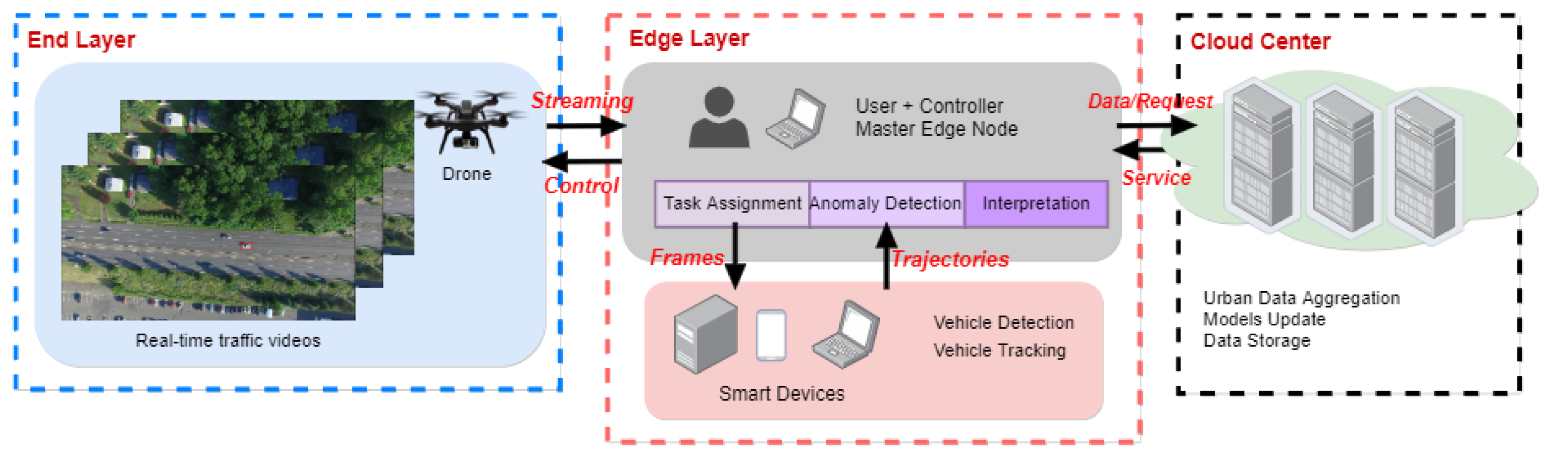
3. SurMon Architecture Overview

Figure 1 presents the overall architecture of the proposed Smart Urban traffic Monitoring (SurMon) system, which includes three layers: end layer, edge layer and cloud layer. End layer consists of smart sensors and devices that collect urban traffic data. In the prototype of the SurMon system, drones are adopted to collect videos over a certain road area in real time, and the h264 coded video streams are transmitted to the ground controller that functions as the edge layer, where compressed video streams get decoded and displayed to the human operator.

While the end layer is in charge of data collection and light-weight data pre-processing tasks, the edge layer operates near-site and performs data analysis for real-time decision-making. Edge computing leverages heterogeneous smart devices as edge nodes. They collaborate with each other to facilitate surveillance tasks with a lower latency. The smart devices include smart phones, tablets, personal laptops, etc. In the SurMon system, major computations take place at the edge layer including vehicle detection, vehicle tracking, anomalous behavior detection, and interpretation. Vehicle detection and tracking tasks extract vehicle trajectories in real time. Due to the resources constraint on smart devices and the complexity of tracking tasks, it entails the collaboration among a number of edge nodes, which are divided into master and slave nodes [69]. The master node orchestrates the collaboration among slave nodes. In the SurMon prototype system, for instance, the in-car user laptop plays the role of the master edge node. It receives video streams from drones and then dispatches decoded video frames to each slave node. Each edge node tracks one single vehicle and transmits the vehicle trajectory data back to the master node for other tasks. Therefore, the computing intensive multi-target tracking task is reformatted as multiple single-target tracking tasks [69]. A task assignment scheme is designed to ensure the synchronization among edge nodes. The video streams from drones are transferred to the ground controller. Once suspicious vehicles are identified, each individual vehicle and the region-of-interest are assigned to a target tracker for consistent tracking and velocity estimation. When more suspicious vehicles are detected, the controller checks with the edge nodes around and dispatches a single target tracking task to one who has sufficient computing power to process the job. Readers who are interested in the details of the rationale and implementation of multiple targets tracking at the edge based on a single target tracking algorithm are referred to [69].

Besides task assignments to each slave node, master node consolidates all trajectories data from each edge node and attempt to detect abnormal driving behaviors and interpret them to decide whether it is appropriate or not. Instead of trying to pre-define driving patterns of abnormal behaviors, SurMon proposes to focus on behaviors that are different from others. Multi-dimensional Singular Spectrum Analysis (mSSA) is adopted to reformulate this problem as a change point detection problem [22]. On the one hand, defining abnormal patterns in advance results in detection inaccuracy since, in practice, it is very difficult to enumerate every abnormal pattern; on the other hand, behaviors that bias away from average patterns are identified first, which effectively reduces computations on edge nodes and the amount of data that is transmitted to a remote cloud center if necessary. However, one trade-off of this approach is that, after the detection of different behaviors, it cannot be simply categorized as aggressive or abnormal driving behaviors in certain situations. For example, in the United States, one of the right-hand drive countries, if a vehicle stops waiting for a left turn while all others are moving forward, this behavior is likely detected and marked as a difference, but it is actually not a violation of traffic rules.

Therefore, to deal with this challenge, a smart traffic surveillance system is necessitated to interpret the detected driving behaviors in a specific context. Due to its superior performance, Capsules Network requires less training data and considers a spatial relationship among features. In the SurMon system, two Capsules Networks, namely CapNet-1 and CapNet-2, are trained with a dataset of good driving behaviors, and they are cascaded together. The CapNet-1 is trained as a multi-class classifier with individual driving behavior data like trajectories, speed, etc. CapNet-1 predicts whether an individual behavior is classified as any of the good ones from the training dataset. CapNet-2 is trained with a set of good driving behaviors in the same time window, and it is a binary classifier that only predicts whether these behaviors agree with each other to formulate a harmony driving scenario. Specifically, the set of the behaviors data goes into CapNet-1 first and then the outputs are taken as the training set for CapNet-2. Within a time window, all vehicle driving behavior data flow into the mSSA for the detection of outliers, and then CapNet-1 takes the detected behavior data and makes the prediction. If it does not fall into any good behavior patterns, all vehicles data are instead fed into CapNet-1, and its output is leveraged by CapNet-2 to predict whether the existence of this abnormal behavior will result in a real negative of a good driving scenario. The basic rationale here is that most vehicles obey the traffic rules and a good driving behavior does not put others at risk.

The last layer of SurMon system is the cloud layer. Meaningful urban data, after being processed at the edge layer, can be transmitted to the cloud for large-scale city-wise traffic pattern recognition. In addition, because of the plentiful computational resources, models can be upgraded in the cloud and then deployed to edge nodes. This paper focuses on the real-time detection and interpretation at the network edge, end layer, and edge layer; the design and experimental studies for the cloud layer are beyond the scope.

The architecture discussed in this section presents the concept and major function blocks. The implementation of an actual SurMon system in the real world depends on many factors, including the budget, the range of the space under surveillance, local traffic regulations, etc. In Section 6, a system configuration of the proof-of-concept prototype for our experimental study is presented.

4. Anomalous Vehicle Behavior Detection Using mSSA

The fundamental idea of the proposed approach lies in an intuitive observation. Most vehicles on roads actually follow traffic rules and behave legitimately. Therefore, vehicles that act significantly different are more likely violating the rules. Consequently, it is reasonable to identify vehicles that present different characteristics from others as objects-of-interest, and more analysis should be conducted on them. The movement of a vehicle can be described using its trajectory information, which consists of an ordered sequence depicting positions, speeds and directions of the vehicle over time. Following this rationale, the anomaly vehicle detection problem is reformatted as a problem of finding the object of changes $v_c$ from the set of objects ${\mathbb{V}}_K$.

For the convenience,

Table 1. Notations used in algorithms.

Notation	Description
${\mathbb{X}}_N$	time series with length N
X	trajectory matrix constructed from ${\mathbb{X}}_N$
${\mathbb{X}}_N^{\left(k\right)}$	time series with k channel
M	window length
l	the number of eigenvalues selected
$X_{base}^{\left(n\right)}$	base matrix at nth iteration
$X_{test}^{\left(n\right)}$	test matrix at nth iteration
${\mathcal{D}}_{n,l,r,s}$	distance between base and test matrix
${\mathcal{X}}_{K,N}^{\left(S\right)}$	time series of S characteristics for K vehicles with length N
${\mathbb{V}}_K$	set of K vehicles
$X_{n,N}^{\left(j\right)}$	trajectory matrix of time series of jth characteristic of nth vehicle
${\mathcal{X}}_{base,N}^{(j,l)}$	base vehicle time series for distance calculation
${\mathcal{D}}_{n,N}^{(j,l)}$	distance from each vehicle to the base vehicle time series
$P_n$	anomaly score for nth vehicle
h	threshold to determine anomalies

summarizes the notations used in this paper.

4.1. A Basic Introduction to SSA

The basic SSA algorithm consists of four steps: embedding, singular value decomposition (SVD), grouping, and diagonal averaging. Let us consider a time series with real values ${\mathbb{X}}_N=(x_1,x_2,\cdots ,x_N)$ with the length of N.

• Embedding: map ${\mathbb{X}}_N$ to a $M\times L$ trajectory matrix X. M is the window length and $L=N-M+1$.

  $$X=[X_1,X_2,\cdots ,X_L]=\left[\begin{array}{cccc}{x}_1& x_2& \cdots & x_L\\ x_2& x_3& \cdots & x_{L+1}\\ ⋮& ⋮& \ddots & ⋮\\ x_M& x_{M+1}& \cdots & x_N\end{array}\right]$$

  (1)

  $$X_i={[x_i,x_{i+1},\dots ,x_{i+M-1}]}^T,i=1,\dots ,L$$

  (2)

  where M is the dimensions of characteristics and L is the number of observations. Trajectory matrix X is a Hankel matrix of which the elements along the anti-diagonals ($i+j=const.$) are the same: $x_{ij}=x_{i+j-1}$. The embedding procedure is a one-to-one mapping.
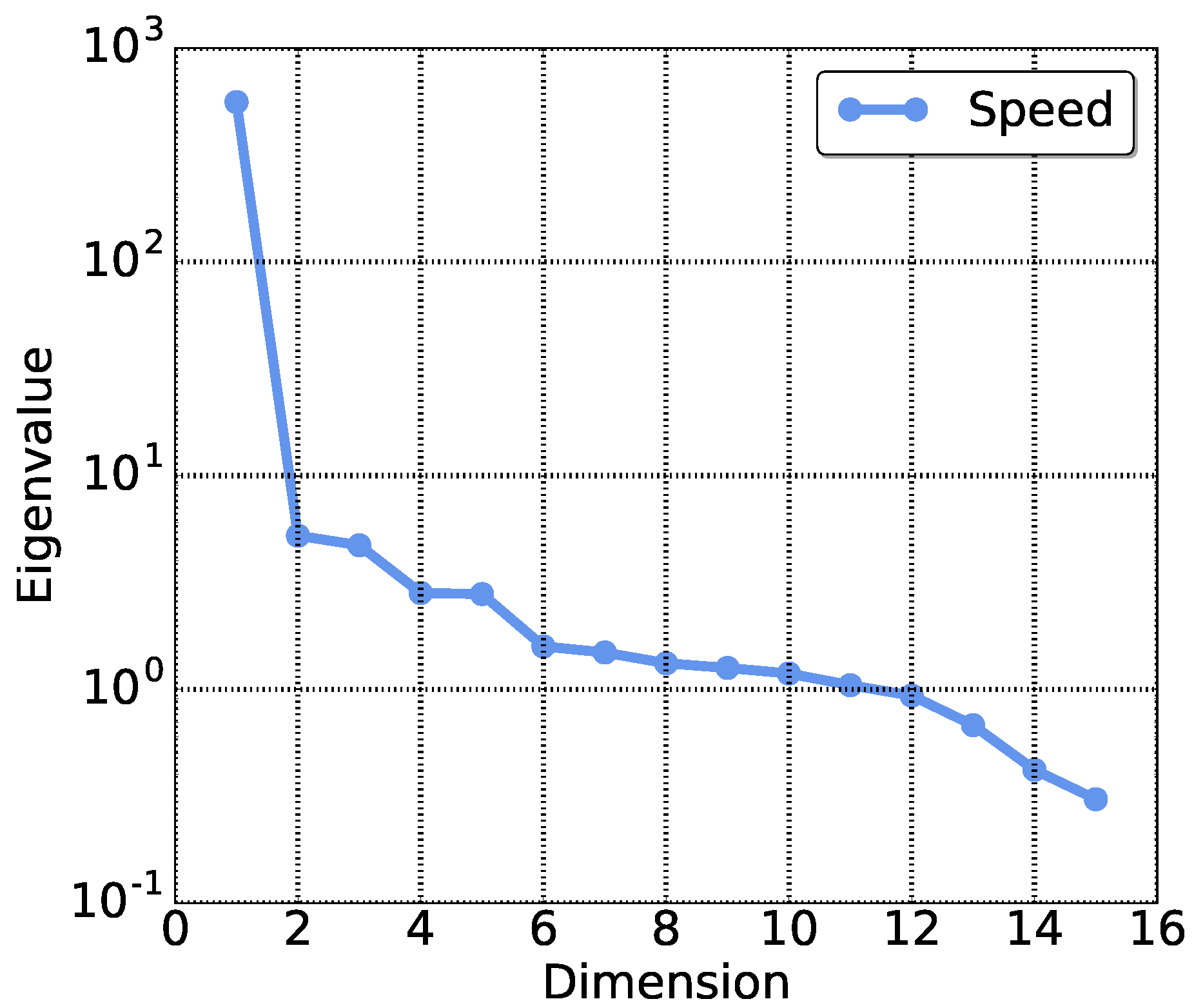
• SVD: the second step is to perform the SVD procedure on the trajectory matrix X. Set covariance matrix $T=X{X}^T$, then its eigenvalues are ${\lambda }_1,{\lambda }_2,\cdots ,{\lambda }_d$ and the corresponding biorthogonal eigenvectors are $U_1,U_2,\cdots ,U_d$, where d is the rank of X. Note that eigenvalues are arranged in a decreasing order and larger than 0. $V_g=X^T{U}_g/\sqrt{{\lambda }_g}$ ($g=1,2,\cdots ,d$); then, the trajectory matrix X can be written as follows:

  $$X=\sum _{g=1}^d{X}_g=\sum _{g=1}^d\sqrt{{\lambda }_g}{U}_g{V}_g^T$$

  (3)

  where $X_g$ is the elementary matrix with rank 1 of the trajectory matrix X, and $V_g$ is one of the eigenvectors of the matrix $S=X^{T}X$.
• Grouping: In the third step, elementary matrices are partitioned into disjoint subsets: $I_1,I_2,\cdots ,I_m$; then, the trajectory matrix X can be rewritten as below. Each subset represents one component of the time series, such as trend, oscillation, or noise.

  $$X=X_{I_1}+X_{I_2}+\cdots +X_{I_m}$$

  (4)
• Diagonal Averaging: in the last step, the reconstruction process maps the matrix with only principal components back to a time series by Hankelizing the matrix $X_l$ with l principal components ($X_l=X_{I_1}+X_{I_2}+\cdots +X_{I_l}$).

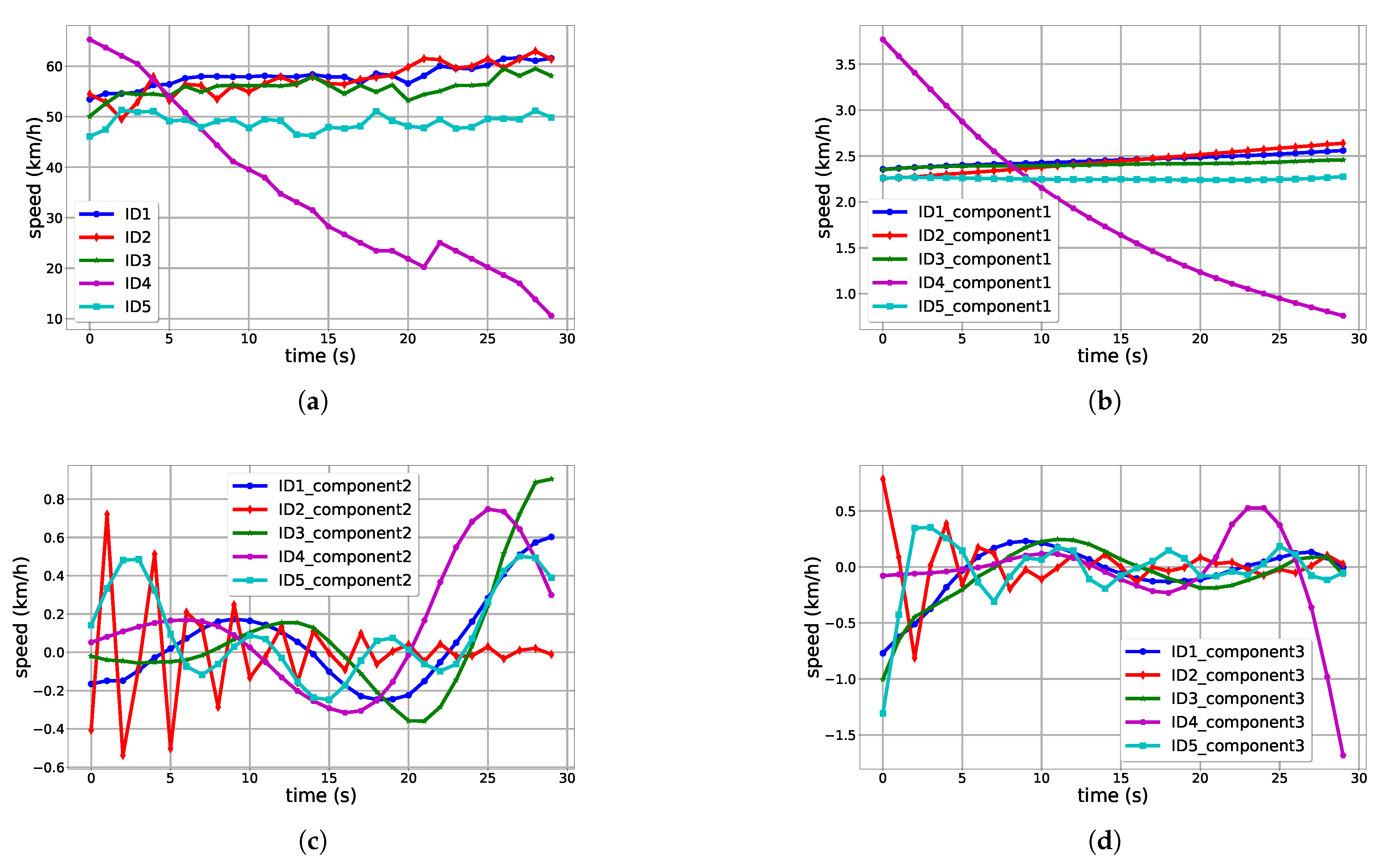
4.2. Multi-Dimensional SSA

The mSSA algorithm analyzes multi-channel time series in the presence of noises. Denote ${\mathbb{X}}_N^{\left(k\right)}$ as k time series with length N of a system. The major difference with basic SSA lies in the trajectory matrix construction step. For channel $X_N^{\left(i\right)}$, where $i=1,\dots ,k$, there is the trajectory matrix with a window length M:

$$X^{\left(i\right)}=[X_1^{\left(i\right)},X_2^{\left(i\right)},\dots ,X_L^{\left(i\right)}],L=N-M+1$$

(5)

Each volume in $X^{\left(i\right)}$ is as follows:

$$X_j^{\left(i\right)}={[x_j^{\left(i\right)},x_{j+1}^{\left(i\right)},\dots ,x_{j+M-1}^{\left(i\right)}]}^T,j=1,\dots ,L$$

(6)

Putting all the trajectory matrices of the time series in each channel together, then

$$X=[X^{\left(1\right)},X^{\left(2\right)},\dots ,X^{\left(k\right)}]$$

(7)

Depending on the application scenarios, as an alternative, trajectory matrices of multiple channel time series can be concatenated vertically. The steps of the mSSA algorithm are the same as the basic SSA procedures.

4.3. SSA-Based Change Point Detection

The original time series can be partitioned into multiple, different components of a time series. With a reasonable grouping strategy, components corresponding to noises or secondary factors can be removed, and only principal components are reserved. Basically, the operation of an SSA based change point detection algorithm is that it moves the sliding window and calculates the distance between the test matrix obtained from the target segmentation of the time series and the base matrix reconstructed from the l-dimensional subspace. An obvious distance between the test matrix and the base matrix will be observed when a change occurs.

Considering a time series, assuming that $N,M,l,r,s$ are fixed integers and n is the iteration step number. Here, N is the segmentation length and M is the window length, $0<M<N/2,0<r<s$. An l dimensional base matrix $X_{base}^{\left(n\right)}$ is constructed by performing the steps one to three: embedding, performing SVD, and grouping. Denote $U_l=[U_1,\cdots ,U_l]$ as the eigenvector subspace composed of the eigenvectors corresponding to first l eigenvalues. Similarly, the test matrix is constructed for the time series segmentation in $[n+r+1,n+s]$:

$$X_{test}^{\left(n\right)}=[X_{n+r+1}^{\left(n\right)},\dots ,X_{n+s}^{\left(n\right)}]$$

(8)

$$X_j^{\left(n\right)}={[X_{n+r+j}^{\left(n\right)},\dots ,X_{n+r+M+j-1}^{\left(n\right)}]}^T$$

(9)

where $j=r+1,\dots ,s$. The size of the test matrix is $M\times (s-r)$.

Next, the Euclidean distance $\mathcal{D}$ between the base matrix and the test matrix is calculated:

$${\mathcal{D}}_{n,l,r,s}=\sum _{j=r+1}^s({(X_i^{\left(n\right)})}^T{X}_i^{\left(n\right)}-{(X_i^{\left(n\right)})}^{T}U{U}^T{X}_i^{\left(n\right)})$$

(10)

where vector $X_j^{\left(n\right)}$ is each column of test matrix $X_{test}^{\left(n\right)}$.

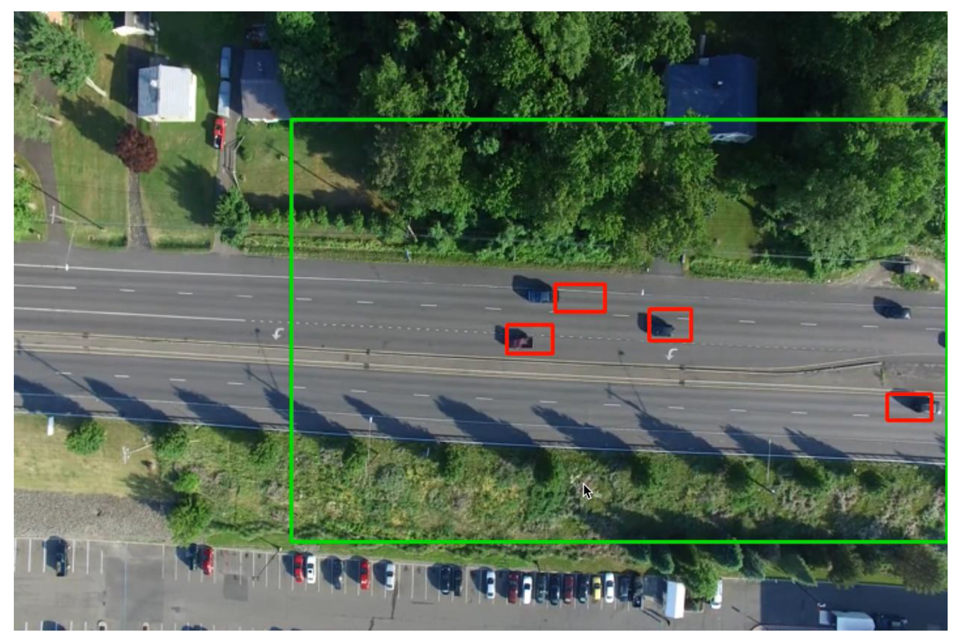
4.4. Detection of Anomalously Behaved Vehicles

The objective of this detection procedure can be described as: given a set of K vehicles ${\mathbb{V}}_K$, identify the vehicle with different behaviors $v_c$. With ${\mathbb{V}}_K$, there are the time sequences of vehicle behavior describing information ${\mathcal{X}}_{K,N}^{\left(S\right)}$. Here, N is the length of time series, and S is the number of features describing the movement of the vehicles. The lengths of trajectories for all vehicles in the set are the same. For every feature of an individual vehicle within the time series length N, a base matrix is constructed. Then, an average of the reconstructed time series of all vehicles represents the average group motion of all the vehicles in the set. Using the average behavior as the base, a distance is calculated from each vehicle. The values of the distances indicate how different one individual behaves from peers.

Just as the steps described earlier, the first step is to embed the time series of each feature for a specific vehicle $v_n$ into a matrix:

$$X_{n,N}^{\left(j\right)}=\left[\begin{array}{cccc}{x}_{n,1}^{\left(j\right)}& x_{n,2}^{\left(j\right)}& \cdots & x_{n,L}^{\left(j\right)}\\ x_{n,2}^{\left(j\right)}& x_{n,3}^{\left(j\right)}& \cdots & x_{n,L+1}^{\left(j\right)}\\ ⋮& ⋮& \ddots & ⋮\\ x_{n,M}^{\left(j\right)}& x_{n,M+1}^{\left(j\right)}& \cdots & x_{n,N}^{\left(j\right)}\end{array}\right]$$

(11)

where $j=1,\dots ,S$, $n=1,\dots ,K$, M is the window length and $L=N-M+1$.

With the matrix $X_{n,N}^{\left(j\right)}$ is obtained, the second step is to perform SVD and select the first $l_j$ eigenvalues to construct the subspace. The subspace closely represents the original time series but ignores the noise and non-significant factors. Denote $U_{l_j}$ as the matrix of which each column is the corresponding eigenvector to the selected eigenvalues. Similarly, $V_{l_j}$ can be calculated.

Next, by reconstructing the time series from the l-dimensional subspace, ${\mathcal{X}}_{n,N}^{(j,l)}$ will be obtained. Then, for each feature, calculate the average of the reconstructed time series of all vehicles to obtain the base matrix:

$${\mathcal{X}}_{base,N}^{(j,l)}=\sum _{n=1}^K{\mathcal{X}}_{n,N}^{(j,l)}/K$$

(12)

The SVD operation is conducted again, but, on this base matrix, an l-dimensional subspace $U_{base,N}^{(j,l)}$ is obtained. Then, each matrix $X_{n,N}^{\left(j\right)}$ is the test matrix of each feature of each individual vehicle, and calculate the distance of the test matrix to this base matrix:

$$\begin{array}{c}\hfill {\mathcal{D}}_{n,N}^{(j,l)}=\sum _{i=1}^L({\left(X_{i,n,N}^{\left(j\right)}\right)}^T{X}_{i,n,N}^{\left(j\right)}-\\ \hfill {\left(X_{i,n,N}^{\left(j\right)}\right)}^T{U}_{base,N}^{(j,l)}{\left(U_{base,N}^{(j,l)}\right)}^T{X}_{i,n,N}^{\left(j\right)}).\end{array}$$

(13)

Normalize the distances within each channel, and then the anomaly score is calculated for each vehicle:

$$P_n=\sum _{j=1}^S{P}_j{\mathcal{D}}_{n,N}^{(j,l)}$$

(14)

where $P_j$ is the weight of each characteristic of the motion of vehicles and ${\sum }_{j=1}^S{P}_j=1$.

A threshold h is pre-set by the system operator either based on past experiences or a certain mathematical analysis. If $P_n>h$, then the n-th vehicle is detected as an anomalous one. It is a complex and challenging process to determine an optimal or suboptimal threshold for SSA algorithms. It is essentially an optimal solution finding problem in high-dimensional space as multiple factors play significant roles, including the window length, number of eigenvalues selected, distance between the base and test matrix, and user expectations. It is worth noting that the trade-offs between the detection delay and the detection accuracy are highly application dependent. A comprehensive discussion is beyond the scope of this paper, and interested readers are referred to [70] for more details.

5. Anomalous Vehicle Behavior Interpretation

5.1. Vehicle Behavior Data

Again, consider a time series with real values ${\mathbb{X}}_N=(x_1,x_2,\cdots ,x_N)$ with the length of N and vehicle behaviors’ characteristics are extracted in different feature channels within a time window; then, a spatial temporal data series of vehicle behaviors with real values in different channels will be:

$${\mathbb{X}}_{n,N}=[x_{n,N}^{\left(1\right)},x_{n,N}^{\left(2\right)},\dots ,x_{n,N}^{\left(k\right)}]$$

(15)

where N denotes the length of a time window, n represents n-th vehicle, and k is the number of channels. The overall length of ${\mathbb{X}}_{n,N}$ is $N\times K$. Then, this spatial temporal series could be converted into a $q\times p$ matrix as:

$$X_{n,N}^{\left(j\right)}=\left[\begin{array}{ccc}{x}_{n,1}^{\left(1\right)}& \cdots & x_{n,p}^{\left(1\right)}\\ ⋮& \ddots & ⋮\\ x_{n,q}^{\left(k\right)}& \cdots & x_{n,N}^{\left(k\right)}\end{array}\right]$$

(16)

where $q\times p=k\times N$. This matrix will be as the input for the cascaded Capsules Network.

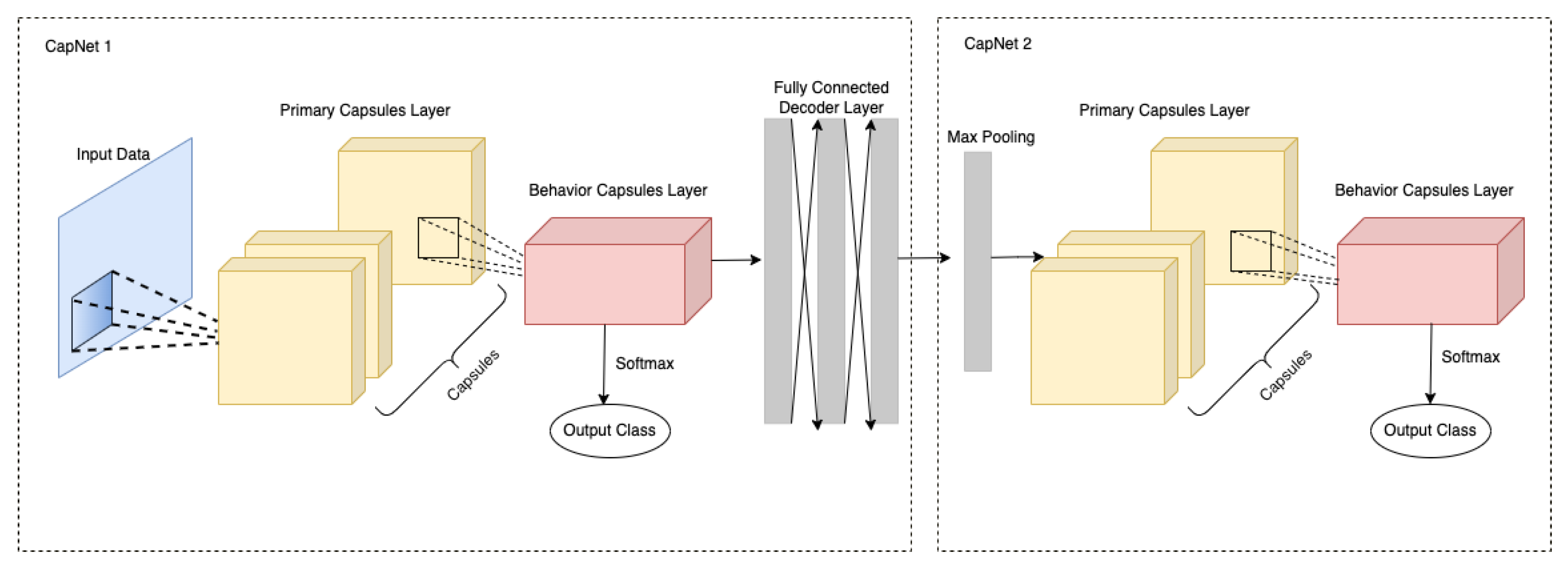
5.2. Cascaded Capsules Network

Capsules are groups of artificial neurons that take vectors as the input and output vectors. The length of the output vectors represents the probabilities of a particular feature that is detected in each capsule. Figure 2 illustrates the overall architecture of the cascaded Capsules Network, which consists of CapNet 1 and CapNet 2. CapNet 1 takes vehicle behavior data as input and predicts if this behavior is one of the normal driving patterns. Otherwise, the outputs of its decoder layer will be fed into CapNet 2. Unlike CapNet 1, CapNet 2 takes multiple vehicle driving behavior data and predicts whether the detected driving behavior will be agreed by others.

5.2.1. CapNet 1

There are three layers in the first Capsules Network of the cascaded approach: primary capsules layer, behavior capsules layer and reconstruction decoder layer.

The vehicle behavior matrix is fed into a convolutional layer first to extract preliminary features. The kernel size is $6\times 6$, and the stride is one. The input channel is equal to one and there are 256 output channels. The primary capsules layer consists of 32 channels of capsules, and each of them has eight convolutional units with kernels of size $9\times 9$, and the stride is equal to two. Then, the output vectors are multiplied by weight matrix $W_{ij}$ and gets summed over with different weights for each channel in a behavior capsules layer:

$$s_j=\sum _i{c}_{ij}{\widehat{\mathit{u}}}_{j|i},{\widehat{\mathit{u}}}_{j|i}={\mathit{W}}_{ij}{\mathit{u}}_i$$

(17)

where $c_{ij}$ is the coupling coefficients between the lower capsules layer and the upper capsules layer, which is determined by the dynamic routing agreement process, and $s_j$ is the input vector of the upper level capsules network, which is a weighted sum over all output vectors ${\widehat{u}}_{j|i}$ from the lower capsules layer.

A squash activation function is applied on $s_j$ to ensure the nonlinearity between different capsules layers:

$$v_j=\frac{{‖{\mathit{s}}_j‖}^2}{1+{‖{\mathit{s}}_j‖}^2}\frac{{\mathit{s}}_j}{‖{\mathit{s}}_j‖}$$

(18)

This activation function maintains the direction of input vectors while the length is normalized. With this squash function, short vectors are closer to zero while long vectors are close to one. The coupling coefficients $c_{i}j$ is calculated by routing softmax:

$$c_{ij}=\frac{exp{b}_{ij}}{{\sum }_{k}exp{b}_{ik}}$$

(19)

where $b_{ij}$ is the logits of the coupling coefficients, which is calculated by the dynamic routing process.

The dynamic routing process is illustrated as Algorithm 1 below. With the dynamic routing algorithm, the scalar product of ${\widehat{\mathit{u}}}_{j|i}{\mathit{v}}_j$ is leveraged to evaluate the agreement between lower level features in primary capsules and high level features in behavior capsules. Then, the agreement is added into $b_{ij}$ to update the coupling coefficients between different capsules layers.

Algorithm 1 Dynamic Routing Algorithm.

ROUTING(${\widehat{\mathit{u}}}_{\mathit{j}|\mathit{i}},r,l$) 2: for all capsule i in layer l and capsule j in layer $(l+1)$: $b_{ij}$← 0     forr iterations do 4:     for all capsule i in layer l: $c_i$ ← $softmax\left(b_i\right)$         for all capsule j in layer $(l+1)$: ${\mathit{s}}_j$ ← ${\sum }_i$$c_{ij}{\widehat{\mathit{u}}}_{j|i}$ 6:     for all capsule j in layer $(l+1)$: ${\mathit{v}}_j$ ← $squash\left({\mathit{s}}_j\right)$         for all capsule i in layer l and capsule j in layer $(l+1)$: $b_{ij}$ ← $b_{ij}+{\widehat{\mathit{u}}}_{j|i}{\mathit{v}}_j$           return ${\mathit{v}}_j$

The $l2$ norm of the output vectors are used to represent the probability of the existence of a capsule entity. The margin loss for class k would be:

$$L_k=T_{k}max(0,m^{+}-‖{\mathbf{v}}_k^2‖)+\lambda (1-T_k)max{(0,‖{\mathbf{v}}_k‖-m^{-})}^2$$

(20)

where $T_k=1$ if the class instantiation exists and $m^{+}=0.9$ while $m^{-}=0.1$. $\lambda$ is set to 0.5 and the total loss becomes the summation of each capsules. Following the behavior Capsules layer, we will check whether the detected behavior falls into any class of normal behaviors. If not, the vehicle driving behavior data will be reconstructed by the reconstruction decoder layer, which consists of three fully connected layers. The size of output matrix is the same as the size of the input matrix.

5.2.2. CapNet 2

There are three layers in the second Capsules Network, CapNet 2, of the cascaded approach: max pooling layer, primary capsules layer, and the behavior capsules layer. The architecture of CapNet 2 in the cascaded approach is the same as CapNet 1 except that, at the beginning, there is a max pooling layer to reduce the size of input matrix. Suppose there are M vehicles detected from road images; then, the input of CapNet 2 is a matrix X with size $M\times N$. Then, let $X_{input}=X^{T}X$, which is the input for a max pooling layer. The kernel size of the max pooling layer is 25, and the stride is 25. After max pooling layer, the structure of CapNet 2 is the same as CapNet 1. The softmax function will be applied to check whether the output falls into the class in which the detected behavior is agreed by others.

6. Experimental Results

6.1. Experimental Setup

A prototype of the proposed SurMon system has been implemented. Two DJI Phantom 3 Professional drones are used to monitor the moving vehicles on the road, and two Nexus 9 tablets are connected to the drone controllers to display the real-time surveillance video. In this prototype, one laptop acts as an edge computing node whose configuration is as follows: the processor is 2.3 GHz Intel Core i7, the RAM memory is 16 GB, and the operating system is OS X EI Capitan. The resolution of video frames is $1280\times 720$. The OpenCV 3.1 and Eigen 3.2.1 are used for the tracking algorithm. The given FOV (field of view) of the camera mounted on the drones is ${94}^{\circ }$, and the actual FOV after calibration is $89.{39}^{\circ }$ according to the fact that manufacturers would always make the image plane not perfectly circumscribed with the CCD plate but a little larger than that.

6.2. mSSA-Based Anomalous Behavior Detection

The proposed mSSA based anomaly detection algorithm is validated using two data sets. One is the video streams that are collected locally using drones as the end layer devices, another is a public data set from the Next Generation Simulation (NGSIM) public Lankershim Boulevard Dataset. In the NGSIM dataset, the vehicle trajectory data were collected on the Lankershim Boulevard in the Universal City neighborhood of Los Angeles on 16 June 2005. A total of 30 min of data are available from 8:30 am to 9:00 a.m. Detailed characteristics of different channels of vehicles trajectory data include spatial information of trajectories in terms of local_x and local_y, vehicle length, vehicle velocity, acceleration, etc. The time interval of each data point is 0.1 s.

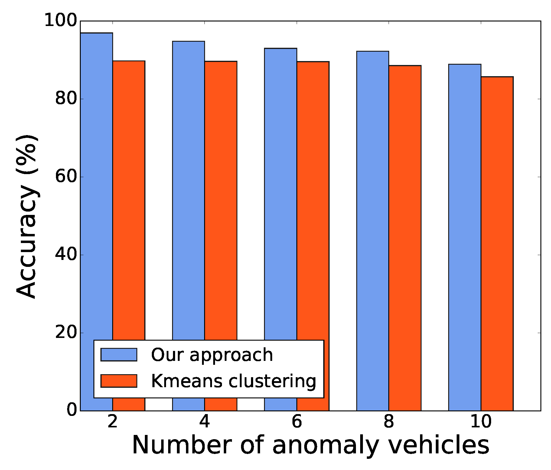
6.2.1. Results with Local Traffic Data

Figure 3 shows an example scenario of the videos collected by the drone overseeing the local traffic. The video streams record the traffic on a road near our campus, which is a local highway with the speed limit of 72 Km/h. For testing purposes, multiple types of anomalous behaviors are created. Three parameters are selected to describe the trajectory for each vehicle: x position and y position of a vehicle in a video frame and the driving speed. The sample frequency on the video is ten samples per second. Five trajectories are selected mainly to validate the feasibility and effectiveness of our method. The five vehicles are labelled as $ID1$, $ID2$, $ID3$, $ID4$, and $ID5$, and the anomalous vehicle is $ID4$.

Grouping is the most important step in the mSSA procedure. Elaborated selections will allow the decomposition of the components of a time series to be conducted efficiently and achieve a higher precision. Figure 4 illustrates the eigenvalues corresponding to the driving speed of vehicle $ID1$. The larger the eigenvalue, the more significant information is contained in the corresponding dimension. In the example shown by Figure 4, the largest eigenvalue is almost ${10}^3$, and all the others stay below ten. This substantial difference leads to the decision that only the largest eigenvalue is applied for reconstruction operation. The others are discarded due to the limited influences.

Figure 5 presents the results of reconstruction for different components of testing trajectories. The time series length N is 30 within three seconds and the window length L is 15. By default, in this paper, the window length L for the construction of the trajectory matrix is set as half of N unless explicitly noted. Figure 5a shows the original speed of the five vehicles. The anomalous vehicle, marked as $ID4$, stops on the road. The curves in Figure 5a verified that the original time series of speed contains noises. The noises mainly result from the vehicle detection algorithms, which are not able to obtain the position information of a vehicle from the same part on the vehicle body in all the frames. Meanwhile, it is very encouraging that the SSA algorithm performs robustly and noises are efficiently attenuated at the grouping step.

In contrast, Figure 5b is the reconstruction result from the subspace that contains only the largest eigenvalue. It is obvious that the interference from noises is removed, and the trend for each vehicle is very clear. After the grouping step, time series for normal vehicles become closer, which is very helpful to increase the detection accuracy. Figure 5c,d show the reconstruction results of the second and third components of the original time series for speed information. The curves in Figure 5c,d do not show a clear trend or any periodic patterns; they change randomly. This result clearly verified the effectiveness of the grouping strategy. It is worth noting the significant distance from $ID4$ to the base (average) that is constructed from all vehicles in the set.

In this experimental study, we have also compared the computation time on two different edge devices. One is a laptop computer with the i7-6820HQ processor, 32 GB memory space, and the maximum frequency is 2.7 GHz. The experimental results show that, when the number of vehicles increases from five to 35, the computing time grows from around 10 ms to almost 100 ms. Since the sampling frequency is still ten samples per second, this performance is sufficient to meet the requirement for anomaly detection in real time. In our data set, with a different number of total vehicles, the percentage of anomaly behaved vehicles is around $20\%$. The time series length N is 30 s. Each data point in the figures is the average of 30 times of tests. The other device adopted in our experiments is a Google Pixel C tablet with a NVIDIA quad processor $X1$, 3 GB RAM, and the maximum frequency is 1.9 GHz. Overall, the computation time is in the range from 100 ms to 900 ms, which is longer than the laptop achieved.

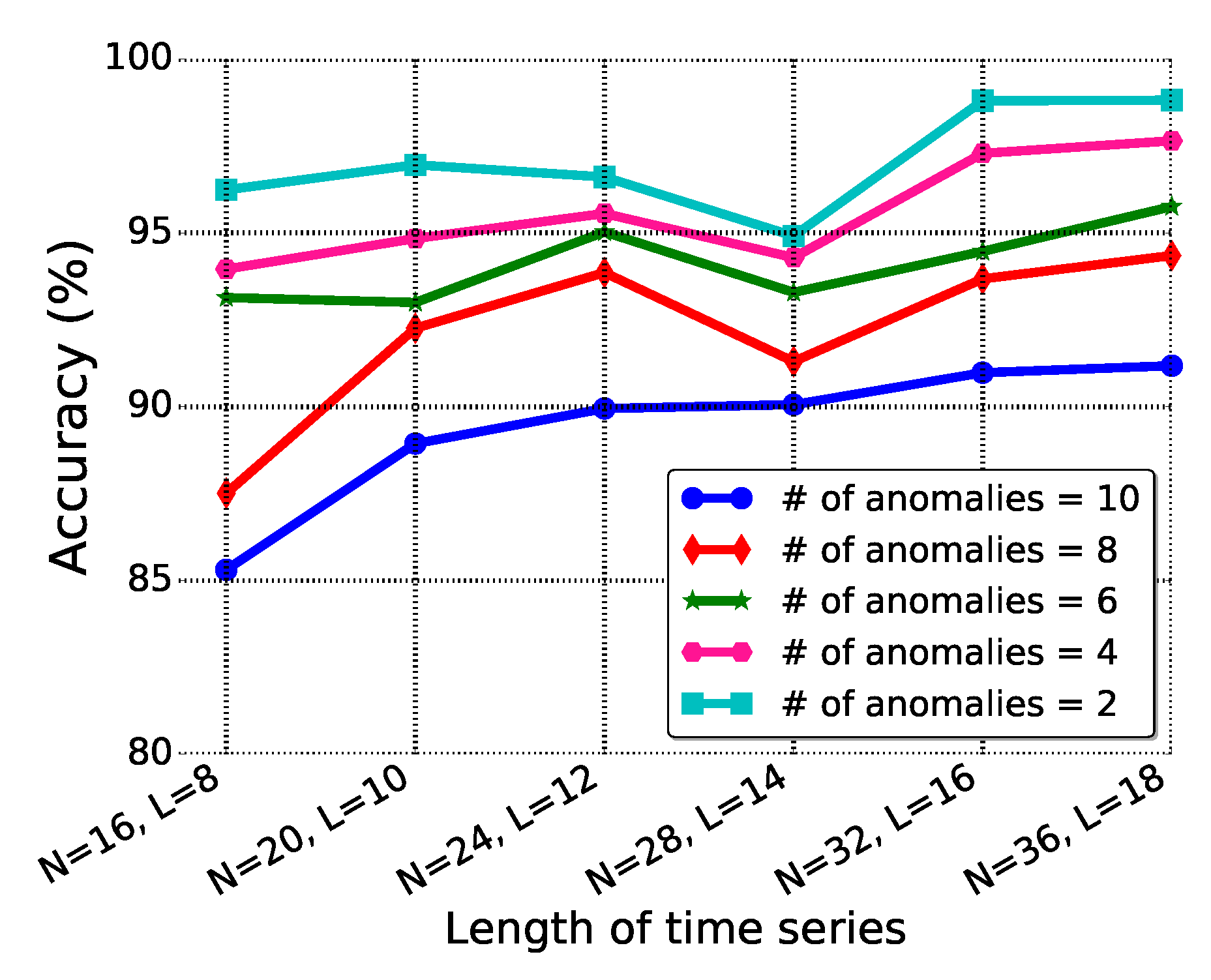
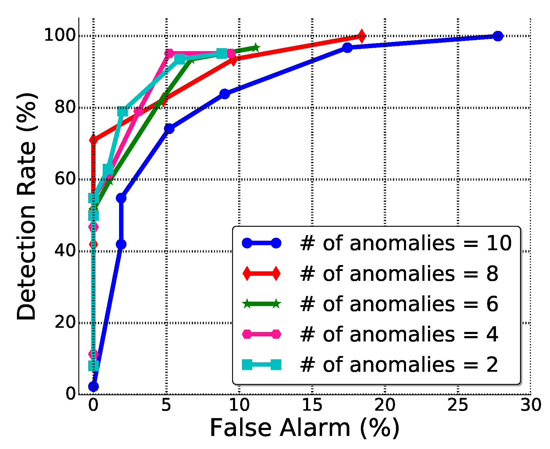
6.2.2. Tests on the Public NGSIM Data Set

A subset is extracted from the NGSIM US-101 data for our experimental study. This subset contains four kinds of vehicle motions, and there are 35 vehicles in total in each video frame, and 50 frames are used in this study. There are two kinds of anomalous vehicle trajectories among the four. The first is one vehicle moving with a much lower speed and the second is that the x position of a vehicle is significantly different from other vehicles. This study compares the mSSA approach with a widely used approach, the KMeans clustering method. Parameters are set as follows: $N=20,L=10,K=2,h=0.5$. K is set as two for clustering: normal and abnormal vehicles. The weights of x, y, and speed are the same.

The experimental results reported in Figure 6 verifies that our mSSA approach outperforms the K-means clustering in terms of detection accuracy. When there are two anomalous vehicles, the mSSA achieves a high detection accuracy of $97\%$. When the number of anomalous vehicles increases, the mSSA maintains a higher detection accuracy than the K-Means clustering method obtained. In this experimental study, a very large percentage of anomalous vehicles was considered, where ten out of 35 vehicles are misbehaved, which is very unlikely to happen in practice. Additionally, the K-Means algorithm can only detect one out the two types of anomalies when the number of anomalous vehicles grows to eight and ten. This comparison study verifies that the similarity based anomaly detection methods always require a thorough prior knowledge about the monitoring scenario and the rules. However, this requirement leads to a poor adaptation for different testing scenarios.

This experimental study also explores the selection of parameters for the mSSA algorithm. With different numbers of misbehaved vehicles among the total 35 vehicles, the window size L and time series length N are investigated to get deeper insight on their impacts on the detection accuracy. The threshold is set as $h=0.5$ based on the experimental experiences with different thresholds. As shown by Figure 7, the time series length N changes from $N=16$ to $N=36$ with iteration 4. With different numbers of misbehaved vehicles, the detection accuracy shows the same trend, going up as N increases.

The experimental study reveals that the proposed mSSA-based anomalous vehicle detection approach is sensitive enough, and it achieves a good performance when the length is the time series is small. The trade-off is, however, that a relatively longer time series provides more information, which potentially will be more reliable in some application scenarios. Hence, N and L should be adjusted accordingly for different scenarios. Meanwhile, larger values of N and L also imply longer detection delays, which must be taken into consideration specifically for delay-sensitive, mission-critical tasks.

Figure 8 plots the ROC curve that illustrates the trade-offs between the false alarm rate and the detection rate. It is very encouraging that, when the detection rate of the proposed approach comes to $100\%$, the false alarm is still low. For example, as shown in Figure 8, when the number of anomalous vehicles is below eight, the operator can set the threshold to get a detection rate of $98\%$, and the false alarm is still below $15\%$.

6.3. CapNet-Based Anomalous Behavior Interpretation

In the experiment, a subset of data from NGSIM is extracted, and vehicle trajectory time series data are from five channels: local_x, local_y, vehicle velocity, vehicle acceleration, and vehicle movement direction.

There are nine sample trajectories in Figure 9 and the legend on the right is vehicle ID. The x-axis and y-axis are the coordinates of vehicle locations within the image. The moving direction is from the top to the bottom. In the recorded video, vehicle 343 made a right turn and vehicles 332, 338, 340, 342, 347, 354, and 355 are going forward in different lanes. Vehicle 345 is the anomalous one. In the video stream, it is observed that vehicle 345 turned left to merge into the lane from a left-turn only exit, which is illegal.

Therefore, the entire subset of trajectories is labeled as five behaviors: turning right, moving forward at lane one, lane two, and lane three, and the last behavior is the abnormal one which is turning left from a wrong exit. There are two capsules networks trained. The CapNet-1 takes individual trajectories as the input, and its training dataset is for four legal driving behaviors except the abnormal one. The goal is to check whether the detected behavior using mSSA can be recognized as any of the normal driving behaviors. The CapNet-2 takes multiple trajectories as the input and is to predict if, with the existence of the detected behavior, it will be agreed by other vehicles.

The time window length is 12.5 s, and there are five channels for each vehicle with different characteristics. The overall length of a trajectory is 625, which will be converted into a $25\times 25$ matrix as the model input. There are 8000 trajectories in the training dataset while the test dataset contains 2000 trajectories. The number of Epoch is six, and the kernel size of the convolutional layer is six with stride one. In the primary capsules layer, there are 32 capsules, and each one contains eight convolutional units. At the behavior capsules layer, there are eight capsules and four classes are for prediction. The model is trained at a virtual machine with 4 GB memory.

Figure 10 shows the training and testing time that is consumed per piece of trajectory data. It takes around 0.225 s to train the model with a trajectory while testing only takes under 0.050 s.

Figure 11 shows the training and testing accuracy. After three epochs, the training accuracy can achieve $100\%$ accuracy. The testing accuracy after epoch three becomes $90\%$ to $100\%$ as well. The experimental results show that the proposed approach can be deployed on edge nodes with limited computational resources and achieve a good performance.

7. Conclusions

In this work, a novel edge computing enabled Smart Urban Traffic Monitoring system named SurMon is investigated. Compared with cloud computing, edge computing facilitates data processing, anomaly detection, pattern recognition, and intelligent decision-making at the network edge with low latency. However, due to the limited computing capabilities of edge nodes, lightweight algorithms are required. A novel mSSA anomaly detection approach is proposed to catch vehicles with abnormal behaviors. Different from traditional ways that identify change points in the time domain, the SurMon system detects anomalies in the space domain. By identifying anomaly vehicles through detecting changes/differences in behaviors, pre-defined normal patterns are not required. Consequently, it relieves the burden of collecting and labelling a huge amount of traffic data, which is relatively labor intensive and impractical. In addition, a cascaded Capsules Network is adopted to interpret these behaviors to decide whether they are legal moves or violations.

A fundamental assumption of our mSSA based anomaly detection algorithm is that most vehicles on roads follow traffic rules and behave legitimately, and outliers are very likely violators. Consequently, it is reasonable to identify vehicles that present different characteristics from others as objects of interest, and more analysis should be conducted on them. In situations where a significant amount or even the majority of the vehicles on the road do not follow traffic rules, our mSSA algorithm may not be an ideal candidate. Meanwhile, a rule-based target-tracking or classification approach using ML is more appropriate.

The results reported here are still at an early stage toward a complete and mature smart urban traffic surveillance application. Several typical driving behaviors are selected to validate the feasibility of the SurMon system. While the experimental results are very encouraging, a lot of open problems are yet to be tackled. In this paper, we focus on the system design, and the experimental study is mainly used to validate the feasibility of the system. Therefore, we tested the effectiveness of mSSA and the multi-target tracking algorithms at the edge for the purpose of suspicious/anomaly vehicles detection, and then switched to the CapNet for behavior Interpretation. Currently, we are extending the implement the CapNet to test its performance on the suspicious behavior detection part, the success of which will provide an alternative solution for devices that are not able to handle the mSSA algorithm.

Our other on-going efforts include mainly two directions. The first is to collect more real-world data and get a comprehensive understanding of the driving behavior on the road. Secondly, since the vehicle information like trajectory is very critical, the security and privacy of driver should not be tampered with. However, edge nodes which facilitate the traffic surveillance tasks will not always be on the white list, and the mobility is also preventing the creation of such a white list. Blockchain is a nice candidate to solve this problem. It allows multiple nodes to reach a consensus within a trustless environment.

References

1. UN. World Urbanization Prospects 2014. 2014. Available online: http://www.un.org/en/development/desa/news/population/world-urbanization-prospects-2014.html (accessed on 9 September 2016).
2. Yannuzzi, M.; van Lingen, F.; Jain, A.; Parellada, O.L.; Flores, M.M.; Carrera, D.; Pérez, J.L.; Montero, D.; Chacin, P.; Corsaro, A.; et al. A new era for cities with fog computing. IEEE Internet Comput. 2017, 21, 54–67. [Google Scholar] [CrossRef]
3. Ullah, F.; Qayyum, S.; Thaheem, M.J.; Al-Turjman, F.; Sepasgozar, S.M. Risk management in sustainable smart cities governance: A TOE framework. Technol. Forecast. Soc. Chang. 2021, 167, 120743. [Google Scholar] [CrossRef]
4. Qian, Y.; Wu, D.; Bao, W.; Lorenz, P. The internet of things for smart cities: Technologies and applications. IEEE Netw. 2019, 33, 4–5. [Google Scholar] [CrossRef]
5. Zhu, Q. Research on road traffic situation awareness system based on image big data. IEEE Intell. Syst. 2019, 35, 18–26. [Google Scholar] [CrossRef]
6. Shahidehpour, M.; Li, Z.; Ganji, M. Smart cities for a sustainable urbanization: Illuminating the need for establishing smart urban infrastructures. IEEE Electrif. Mag. 2018, 6, 16–33. [Google Scholar] [CrossRef]
7. Visvizi, A.; Lytras, M.D. Sustainable Smart Cities and Smart Villages Research: Rethinking Security, Safety, Well-Being, and Happiness. Sustainability 2020, 12, 215. [Google Scholar] [CrossRef] [Green Version]
8. Chackravarthy, S.; Schmitt, S.; Yang, L. Intelligent crime anomaly detection in smart cities using deep learning. In Proceedings of the 2018 IEEE 4th International Conference on Collaboration and Internet Computing (CIC), Philadelphia, PA, USA, 18–20 October 2018; IEEE: Piscataway, NJ, USA, 2018; pp. 399–404. [Google Scholar]
9. Unions, U. World Health Organization: Road Traffic Deaths. Available online: https://sdgs.un.org/goals/goal11 (accessed on 25 October 2021).
10. Cao, K.; Liu, Y.; Meng, G.; Sun, Q. An overview on edge computing research. IEEE Access 2020, 8, 85714–85728. [Google Scholar] [CrossRef]
11. Kuang, L.; Gong, T.; OuYang, S.; Gao, H.; Deng, S. Offloading decision methods for multiple users with structured tasks in edge computing for smart cities. Future Gener. Comput. Syst. 2020, 105, 717–729. [Google Scholar] [CrossRef]
12. Chen, N.; Chen, Y. Smart city surveillance at the network edge in the era of iot: Opportunities and challenges. In Smart Cities; Springer: Berlin/Heidelberg, Germany, 2018; pp. 153–176. [Google Scholar] [CrossRef]
13. Ghosh, A.M.; Grolinger, K. Edge-cloud computing for Internet of Things data analytics: Embedding intelligence in the edge with deep learning. IEEE Trans. Ind. Inform. 2020, 17, 2191–2200. [Google Scholar]
14. Shi, W.; Cao, J.; Zhang, Q.; Li, Y.; Xu, L. Edge computing: Vision and challenges. IEEE Internet Things J. 2016, 3, 637–646. [Google Scholar] [CrossRef]
15. Xu, R.; Nikouei, S.Y.; Chen, Y.; Polunchenko, A.; Song, S.; Deng, C.; Faughnan, T.R. Real-time human objects tracking for smart surveillance at the edge. In Proceedings of the 2018 IEEE International Conference on Communications (ICC), Kansas City, MO, USA, 20–24 May 2018; IEEE: Piscataway, NJ, USA, 2018; pp. 1–6. [Google Scholar]
16. Yun, K.; Huyen, A.; Lu, T. Deep neural networks for pattern recognition. arXiv 2018, arXiv:1809.09645. [Google Scholar]
17. Wang, X.; Han, Y.; Leung, V.C.; Niyato, D.; Yan, X.; Chen, X. Convergence of edge computing and deep learning: A comprehensive survey. IEEE Commun. Surv. Tutor. 2020, 22, 869–904. [Google Scholar] [CrossRef] [Green Version]
18. Zhao, Z.; Barijough, K.M.; Gerstlauer, A. Deepthings: Distributed adaptive deep learning inference on resource-constrained iot edge clusters. IEEE Trans. Comput. Aided Des. Integr. Circuits Syst. 2018, 37, 2348–2359. [Google Scholar] [CrossRef]
19. Teerapittayanon, S.; McDanel, B.; Kung, H.T. Distributed deep neural networks over the cloud, the edge and end devices. In Proceedings of the 2017 IEEE 37th International Conference on Distributed Computing Systems (ICDCS), Atlanta, GA, USA, 5–8 June 2017; IEEE: Piscataway, NJ, USA, 2017; pp. 328–339. [Google Scholar]
20. Sabour, S.; Frosst, N.; Hinton, G.E. Dynamic routing between capsules. arXiv 2017, arXiv:1710.09829. [Google Scholar]
21. Punjabi, A.; Schmid, J.; Katsaggelos, A.K. Examining the benefits of capsule neural networks. arXiv 2020, arXiv:2001.10964. [Google Scholar]
22. Chen, N.; Yang, Z.; Chen, Y.; Polunchenko, A. Online anomalous vehicle detection at the edge using multidimensional SSA. In Proceedings of the 2017 IEEE Conference on Computer Communications Workshops (INFOCOM WKSHPS), Atlanta, GA, USA, 1–4 May 2017; IEEE: Piscataway, NJ, USA, 2017; pp. 851–856. [Google Scholar]
23. Department of Transportation ITS Joint Program Office. New Data Sets from the Next Generation Simulation (NGSIM) Program are Now Available in the Research Data Exchange (RDE). Available online: http://www.its.dot.gov/press/2016/datasets_ngsim.htm (accessed on 22 December 2021).
24. Dong, Q.; Yang, Z.; Chen, Y.; Li, X.; Zeng, K. Exploration of singular spectrum analysis for online anomaly detection in crns. EAI Endorsed Trans. Secur. Saf. 2017, 4, e3. [Google Scholar] [CrossRef] [Green Version]
25. Cai, Y.; Wang, H.; Chen, X.; Jiang, H. Trajectory-based anomalous behaviour detection for intelligent traffic surveillance. IET Intell. Transp. Syst. 2015, 9, 810–816. [Google Scholar] [CrossRef]
26. Wu, C.E.; Yang, W.Y.; Ting, H.C.; Wang, J.S. Traffic pattern modeling, trajectory classification and vehicle tracking within urban intersections. In Proceedings of the 2017 International Smart Cities Conference (ISC2), Wuxi, China, 14–17 September 2017; IEEE: Piscataway, NJ, USA, 2017; pp. 1–6. [Google Scholar]
27. Santhosh, K.K.; Dogra, D.P.; Roy, P.P. Anomaly detection in road traffic using visual surveillance: A survey. ACM Comput. Surv. (CSUR) 2020, 53, 1–26. [Google Scholar] [CrossRef]
28. Ucar, S.; Patnayak, C.; Oza, P.; Hoh, B.; Oguchi, K. Management of Anomalous Driving Behavior. In Proceedings of the 2019 IEEE Vehicular Networking Conference (VNC), Los Angeles, CA, USA, 4–9 December 2019; IEEE: Piscataway, NJ, USA, 2019; pp. 1–4. [Google Scholar]
29. Lefkopoulos, V.; Menner, M.; Domahidi, A.; Zeilinger, M.N. Interaction-aware motion prediction for autonomous driving: A multiple model kalman filtering scheme. IEEE Robot. Autom. Lett. 2020, 6, 80–87. [Google Scholar] [CrossRef]
30. Mozaffari, S.; Al-Jarrah, O.Y.; Dianati, M.; Jennings, P.; Mouzakitis, A. Deep learning-based vehicle behavior prediction for autonomous driving applications: A review. IEEE Trans. Intell. Transp. Syst. 2020, 23, 33–47. [Google Scholar] [CrossRef]
31. Hu, J.; Zhang, X.; Maybank, S. Abnormal driving detection with normalized driving behavior data: A deep learning approach. IEEE Trans. Veh. Technol. 2020, 69, 6943–6951. [Google Scholar] [CrossRef]
32. Xun, Y.; Qin, J.; Liu, J. Deep Learning Enhanced Driving Behavior Evaluation Based on Vehicle-Edge-Cloud Architecture. IEEE Trans. Veh. Technol. 2021, 70, 6172–6177. [Google Scholar] [CrossRef]
33. Wang, J.; Wang, M.; Liu, Q.; Yin, G.; Zhang, Y. Deep anomaly detection in expressway based on edge computing and deep learning. J. Ambient. Intell. Humaniz. Comput. 2020, 1–13. [Google Scholar] [CrossRef]
34. Jiang, L.; Xie, W.; Zhang, D.; Gu, T. Smart diagnosis: Deep learning boosted driver inattention detection and abnormal driving prediction. IEEE Internet Things J. 2021, 1–14. [Google Scholar] [CrossRef]
35. Chen, J.; Ran, X. Deep Learning With Edge Computing: A Review. Proc. IEEE 2019, 107, 1655–1674. [Google Scholar] [CrossRef]
36. Li, H.; Ota, K.; Dong, M. Learning IoT in edge: Deep learning for the Internet of Things with edge computing. IEEE Netw. 2018, 32, 96–101. [Google Scholar] [CrossRef] [Green Version]
37. Qi, X.; Liu, C. Enabling deep learning on iot edge: Approaches and evaluation. In Proceedings of the 2018 IEEE/ACM Symposium on Edge Computing (SEC), Seattle, WA, USA, 25–27 October 2018; IEEE: Piscataway, NJ, USA, 2018; pp. 367–372. [Google Scholar]
38. Liu, W.; Anguelov, D.; Erhan, D.; Szegedy, C.; Reed, S.; Fu, C.Y.; Berg, A.C. Ssd: Single shot multibox detector. In European Conference on Computer Vision; Springer: Berlin/Heidelberg, Germany, 2016; pp. 21–37. [Google Scholar]
39. Redmon, J.; Farhadi, A. Yolov3: An incremental improvement. arXiv 2018, arXiv:1804.02767. [Google Scholar]
40. Howard, A.G.; Zhu, M.; Chen, B.; Kalenichenko, D.; Wang, W.; Weyand, T.; Andreetto, M.; Adam, H. Mobilenets: Efficient convolutional neural networks for mobile vision applications. arXiv 2017, arXiv:1704.04861. [Google Scholar]
41. Liang, T.; Glossner, J.; Wang, L.; Shi, S.; Zhang, X. Pruning and quantization for deep neural network acceleration: A survey. Neurocomputing 2021, 461, 370–403. [Google Scholar] [CrossRef]
42. Liu, S.; Lin, Y.; Zhou, Z.; Nan, K.; Liu, H.; Du, J. On-demand deep model compression for mobile devices: A usage-driven model selection framework. In Proceedings of the 16th Annual International Conference on Mobile Systems, Applications, and Services, Munich, Germany, 10–15 June 2018; pp. 389–400. [Google Scholar]
43. Yao, S.; Zhao, Y.; Zhang, A.; Su, L.; Abdelzaher, T. Deepiot: Compressing deep neural network structures for sensing systems with a compressor-critic framework. In Proceedings of the 15th ACM Conference on Embedded Network Sensor Systems, Delft, The Netherlands, 6–8 November 2017; pp. 1–14. [Google Scholar]
44. Reuther, A.; Michaleas, P.; Jones, M.; Gadepally, V.; Samsi, S.; Kepner, J. AI Accelerator Survey and Trends. In Proceedings of the 2021 IEEE High Performance Extreme Computing Conference (HPEC), Waltham, MA, USA, 21–23 September 2021; IEEE: Piscataway, NJ, USA, 2021; pp. 1–9. [Google Scholar]
45. Machupalli, R.; Hossain, M.; Mandal, M. Review of ASIC Accelerators for Deep Neural Network. Microprocess. Microsyst. 2022, 89, 104441. [Google Scholar] [CrossRef]
46. Shawahna, A.; Sait, S.M.; El-Maleh, A. FPGA-based accelerators of deep learning networks for learning and classification: A review. IEEE Access 2018, 7, 7823–7859. [Google Scholar] [CrossRef]
47. Guo, H.; Liu, J.; Lv, J. Toward intelligent task offloading at the edge. IEEE Netw. 2019, 34, 128–134. [Google Scholar] [CrossRef]
48. Yu, S.; Chen, X.; Yang, L.; Wu, D.; Bennis, M.; Zhang, J. Intelligent edge: Leveraging deep imitation learning for mobile edge computation offloading. IEEE Wirel. Commun. 2020, 27, 92–99. [Google Scholar] [CrossRef]
49. Zamzam, M.; Elshabrawy, T.; Ashour, M. Resource management using machine learning in mobile edge computing: A survey. In Proceedings of the 2019 Ninth International Conference on Intelligent Computing and Information Systems (ICICIS), Cairo, Egypt, 8–12 December 2019; IEEE: Piscataway, NJ, USA, 2019; pp. 112–117. [Google Scholar]
50. Jiang, J.; Ananthanarayanan, G.; Bodik, P.; Sen, S.; Stoica, I. Chameleon: Scalable adaptation of video analytics. In Proceedings of the 2018 Conference of the ACM Special Interest Group on Data Communication, Budapest, Hungary, 20–25 August 2018; pp. 253–266. [Google Scholar]
51. Park, J.; Samarakoon, S.; Elgabli, A.; Kim, J.; Bennis, M.; Kim, S.L.; Debbah, M. Communication-efficient and distributed learning over wireless networks: Principles and applications. Proc. IEEE 2021, 109, 796–819. [Google Scholar] [CrossRef]
52. Kang, Y.; Hauswald, J.; Gao, C.; Rovinski, A.; Mudge, T.; Mars, J.; Tang, L. Neurosurgeon: Collaborative intelligence between the cloud and mobile edge. ACM SIGARCH Comput. Archit. News 2017, 45, 615–629. [Google Scholar] [CrossRef] [Green Version]
53. Ran, X.; Chen, H.; Zhu, X.; Liu, Z.; Chen, J. Deepdecision: A mobile deep learning framework for edge video analytics. In Proceedings of the IEEE INFOCOM 2018-IEEE Conference on Computer Communications, Honolulu, HI, USA, 15–19 April 2018; IEEE: Piscataway, NJ, USA, 2018; pp. 1421–1429. [Google Scholar]
54. Raza, A.; Huo, H.; Sirajuddin, S.; Fang, T. Diverse capsules network combining multiconvolutional layers for remote sensing image scene classification. IEEE J. Sel. Top. Appl. Earth Obs. Remote Sens. 2020, 13, 5297–5313. [Google Scholar] [CrossRef]
55. Afshar, P.; Mohammadi, A.; Plataniotis, K.N. Brain tumor type classification via capsule networks. In Proceedings of the 2018 25th IEEE International Conference on Image Processing (ICIP), Athens, Greece, 7–10 October 2018; IEEE: Piscataway, NJ, USA, 2018; pp. 3129–3133. [Google Scholar]
56. Guo, Y.; Pan, Z.; Wang, M.; Wang, J.; Yang, W. Learning capsules for SAR target recognition. IEEE J. Sel. Top. Appl. Earth Obs. Remote Sens. 2020, 13, 4663–4673. [Google Scholar] [CrossRef]
57. Chen, R.; Jalal, M.A.; Mihaylova, L.; Moore, R.K. Learning capsules for vehicle logo recognition. In Proceedings of the 2018 21st International Conference on Information Fusion (FUSION), Cambridge, UK, 10–13 July 2018; IEEE: Piscataway, NJ, USA, 2018; pp. 565–572. [Google Scholar]
58. LaLonde, R.; Xu, Z.; Irmakci, I.; Jain, S.; Bagci, U. Capsules for biomedical image segmentation. Med. Image Anal. 2021, 68, 101889. [Google Scholar] [CrossRef]
59. LaLonde, R.; Bagci, U. Capsules for object segmentation. arXiv 2018, arXiv:1804.04241. [Google Scholar]
60. Weld, H.; Huang, X.; Long, S.; Poon, J.; Han, S.C. A survey of joint intent detection and slot-filling models in natural language understanding. arXiv 2021, arXiv:2101.08091. [Google Scholar]
61. Staliūnaitė, I.; Iacobacci, I. Auxiliary Capsules for Natural Language Understanding. In Proceedings of the ICASSP 2020-2020 IEEE International Conference on Acoustics, Speech and Signal Processing (ICASSP), Barcelona, Spain, 4–8 May 2020; IEEE: Piscataway, NJ, USA, 2020; pp. 8154–8158. [Google Scholar]
62. Tsangouri, E.; Lelon, J.; Minnebo, P.; Asaue, H.; Shiotani, T.; Van Tittelboom, K.; De Belie, N.; Aggelis, D.G.; Van Hemelrijck, D. Feasibility study on real-scale, self-healing concrete slab by developing a smart capsules network and assessed by a plethora of advanced monitoring techniques. Constr. Build. Mater. 2019, 228, 116780. [Google Scholar] [CrossRef]
63. Patrick, M.K.; Adekoya, A.F.; Mighty, A.A.; Edward, B.Y. Capsule networks—A survey. J. King Saud Univ. Comput. Inf. Sci. 2022, 34, 1295–1310. [Google Scholar]
64. Zhao, A.; Dong, J.; Li, J.; Qi, L.; Zhou, H. Associated Spatio-Temporal Capsule Network for Gait Recognition. IEEE Trans. Multimed. 2021, 24, 846–860. [Google Scholar] [CrossRef]
65. Paik, I.; Kwak, T.; Kim, I. Capsule networks need an improved routing algorithm. In Proceedings of the Asian Conference on Machine Learning, PMLR, Nagoya, Japan, 17–19 November 2019; pp. 489–502. [Google Scholar]
66. Li, D.; Lin, C.; Gao, W.; Chen, Z.; Wang, Z.; Liu, G. Capsules TCN network for urban computing and intelligence in urban traffic prediction. Wirel. Commun. Mob. Comput. 2020, 2020, 6896579. [Google Scholar] [CrossRef]
67. Ma, X.; Zhong, H.; Li, Y.; Ma, J.; Cui, Z.; Wang, Y. Forecasting transportation network speed using deep capsule networks with nested LSTM models. IEEE Trans. Intell. Transp. Syst. 2020, 22, 4813–4824. [Google Scholar] [CrossRef] [Green Version]
68. Kim, Y.; Wang, P.; Zhu, Y.; Mihaylova, L. A capsule network for traffic speed prediction in complex road networks. In Proceedings of the 2018 Sensor Data Fusion: Trends, Solutions, Applications (SDF), Bonn, Germany, 9–11 October 2018; IEEE: Piscataway, NJ, USA, 2018; pp. 1–6. [Google Scholar]
69. Chen, N.; Chen, Y.; Blasch, E.; Ling, H.; You, Y.; Ye, X. Enabling smart urban surveillance at the edge. In Proceedings of the 2017 IEEE International Conference on Smart Cloud (SmartCloud), New York, NY, USA, 3–5 November 2017; IEEE: Piscataway, NJ, USA, 2017; pp. 109–119. [Google Scholar]
70. Xie, L.; Zou, S.; Xie, Y.; Veeravalli, V.V. Sequential (Quickest) Change Detection: Classical Results and New Directions. IEEE J. Sel. Areas Inf. Theory 2021, 2, 494–514. [Google Scholar] [CrossRef]
Figure 1. Overview of the SurMon framework.
Futureinternet 14 00054 g001
Figure 2. Architecture of the Cascaded Capsules Network.
Futureinternet 14 00054 g002
Figure 3. An example traffic scenario collected by the drone.
Futureinternet 14 00054 g003
Figure 4. Eigenvalues for different dimensions.
Futureinternet 14 00054 g004
Figure 5. Components of testing vehicle trajectories. (a) Original speed data sequence; (b) The first component; (c) The second component; (d) The third component.
Futureinternet 14 00054 g005
Figure 6. Detection accuracy comparison.
Futureinternet 14 00054 g006
Figure 7. Detection accuracy for different length N.
Futureinternet 14 00054 g007
Figure 8. ROC curve.
Futureinternet 14 00054 g008
Figure 9. Sample trajectories from the NGSIM data set.
Futureinternet 14 00054 g009
Figure 10. Training and testing time.
Futureinternet 14 00054 g010
Figure 11. Training and testing accuracy.
Futureinternet 14 00054 g011