
A Comparative Study on Traffic Modeling Techniques for Predicting and Simulating Traffic Behavior


Abstract
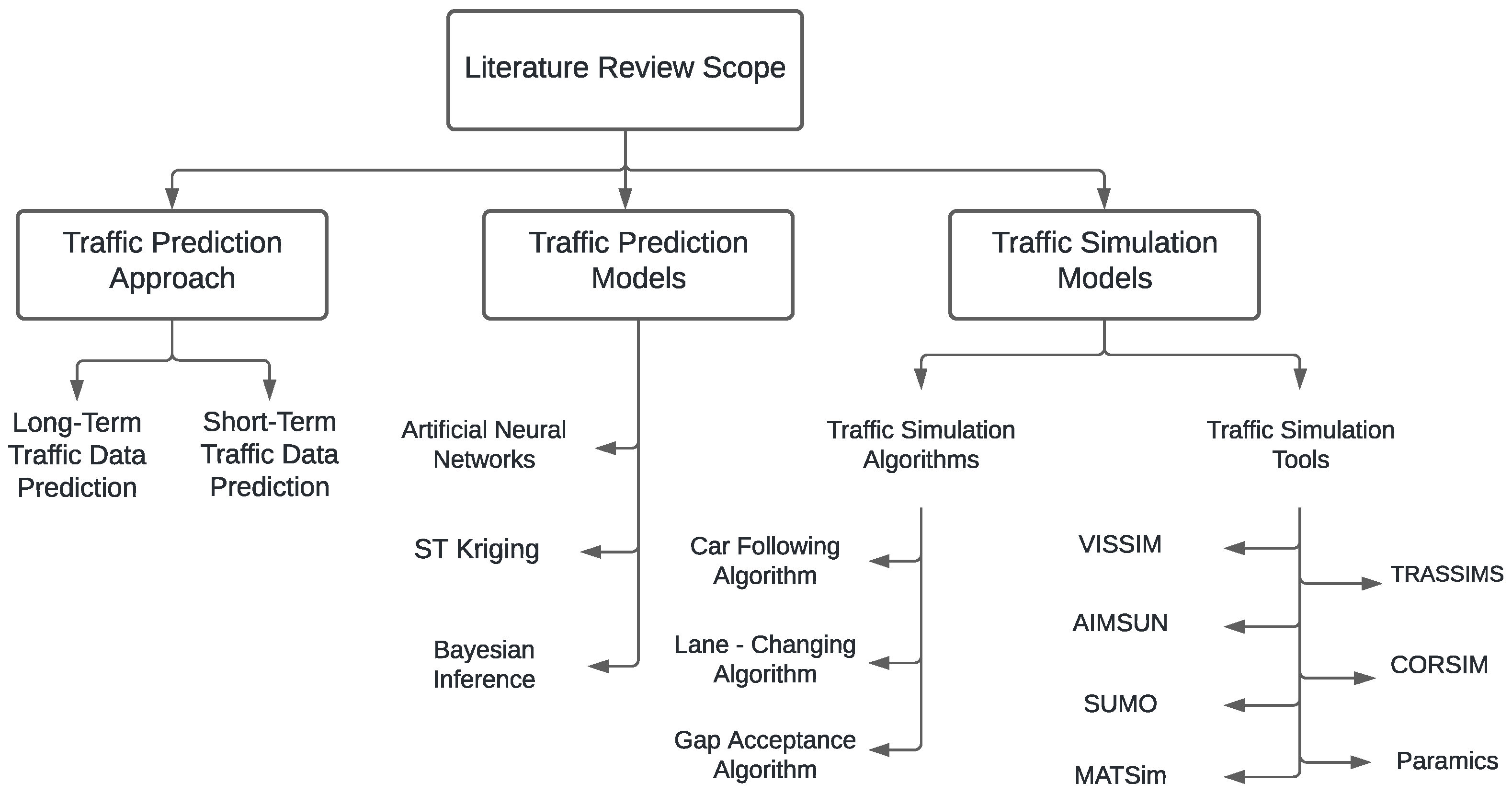
1. Introduction
2. Motivations
3. Traffic Status Prediction
3.1. Short-Term Traffic Prediction
3.2. Long-Term Traffic Data Prediction
3.3. Challenges in Traffic Prediction
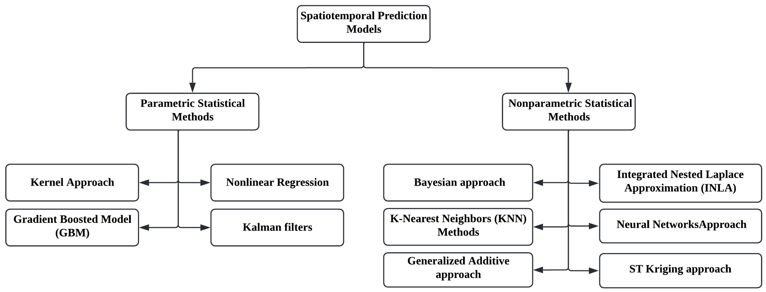
4. Spatiotemporal Traffic Prediction Models
4.1. The ST-Kriging Approach
4.2. Bayesian Inference Approach
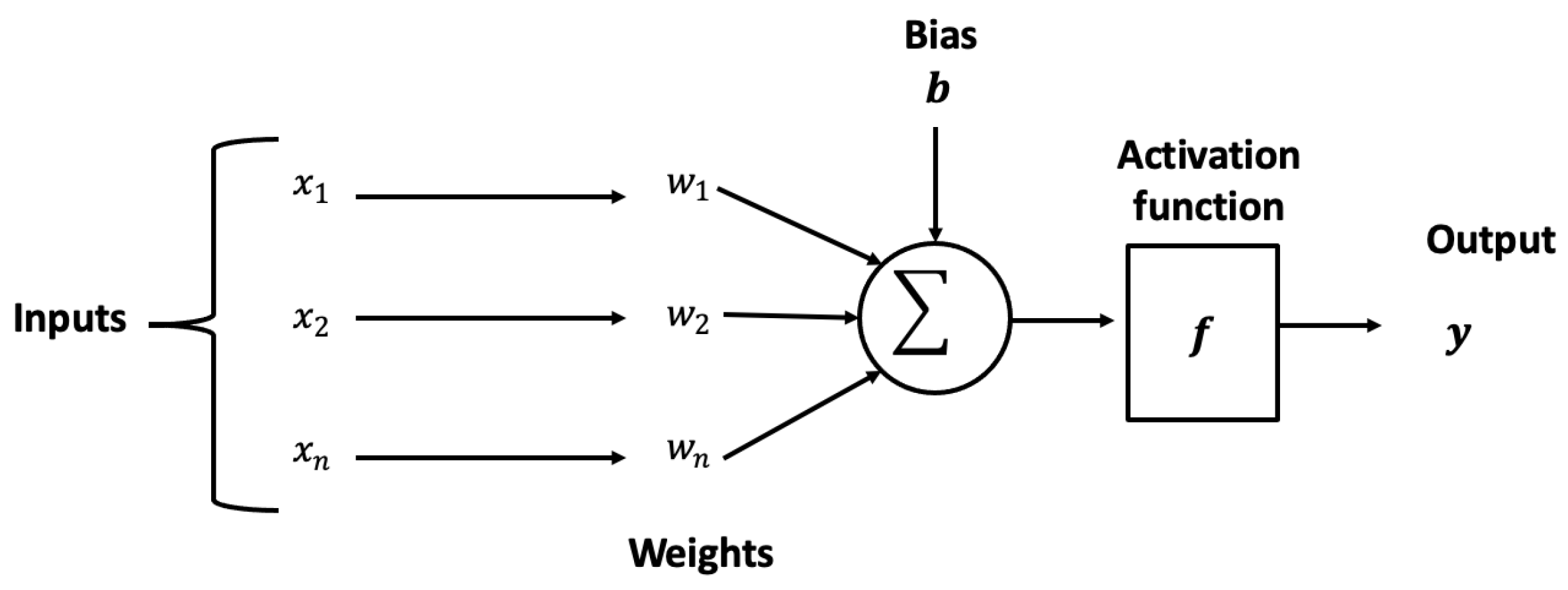
4.3. The Artificial Neural Network Approach
4.4. Summary of Spatiotemporal Traffic Prediction Models
5. Traffic Simulation Models
5.1. Traffic Simulation Algorithms
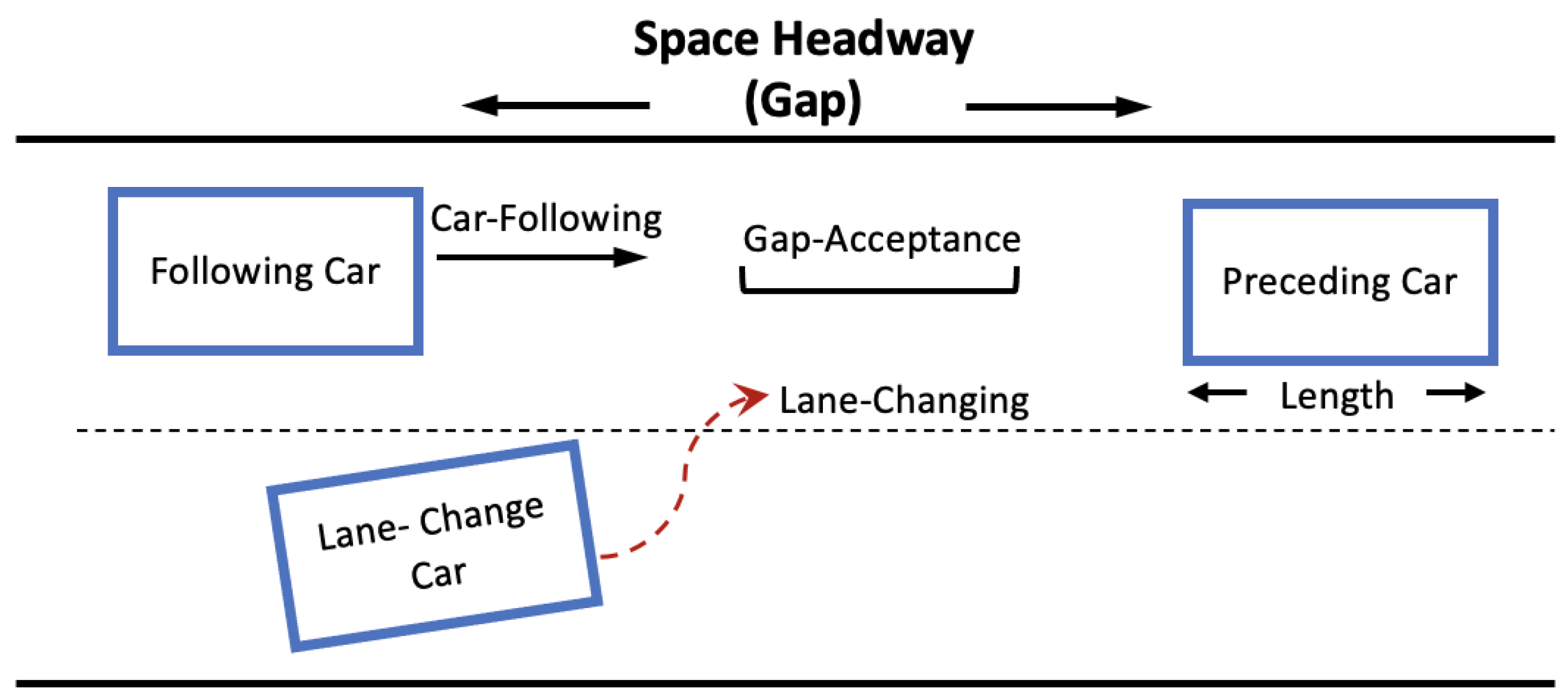
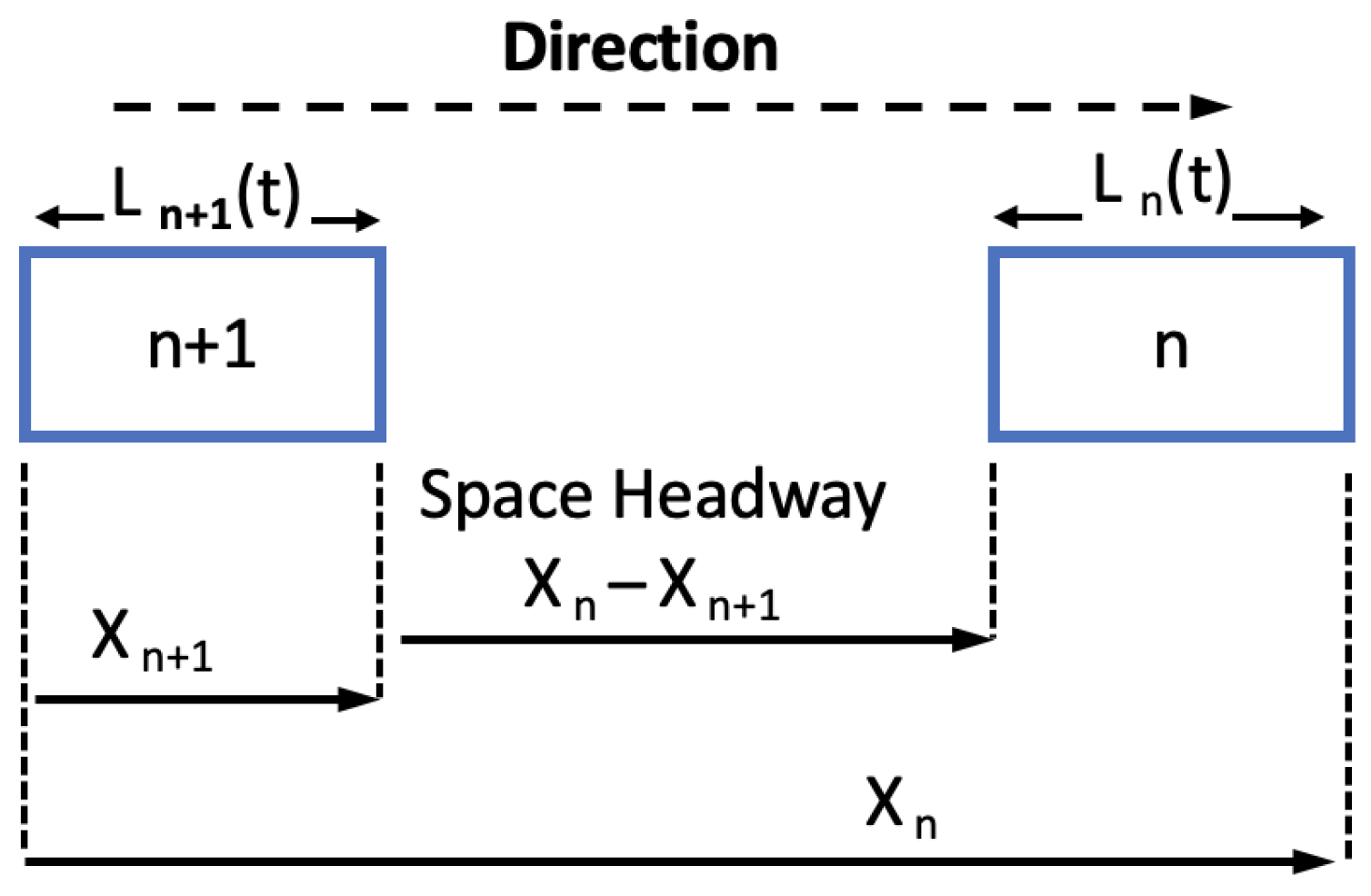
- Car following models: A car-following algorithm is intended to describe how the simulated vehicles interact with the preceding vehicle in the same lane. For any car-following algorithm, the basic parameters used to define the speed–spacing relations are the capacity of a lane, the speed, and the average spacing between the preceding vehicle and the following vehicle [67]. Let n be the preceding vehicle, and be the following vehicle with a speed s and vehicle position x at time t. Therefore, the speed and position of the preceding vehicle are denoted by and , respectively. Similarly, the speed and position of the following vehicle are given by and , respectively [66,68]. The acceleration in speed is denoted by at time t, and the difference in speed between the preceding and the following vehicle is denoted by . Let t+ be the time period when the vehicle accelerates, where is the time required for the driver to respond to a changing scenario. As a result, the safe distance between the preceding and the following vehicle is computed as , which we refer to as the space headway . Let be the sensitivity coefficient parameter that is estimated by modeling the sensitivity of the relative distance between the following and preceding vehicles as well as the sensitivity of the relative speed for the subject vehicle [67,69]. The notations used to describe the car-following algorithm are shown in Figure 5, and the basic equation of the car-following algorithm can be represented as follows:Let be the sensitivity coefficient parameter that is estimated by modeling the sensitivity of the relative distance between the following and preceding vehicles, as well as the sensitivity of the relative speed for the subject vehicle.Figure 5. Basic car-following model.
 In traffic simulators, car-following algorithms adopt exact replicas of the car-following maneuvers which are carried out by drivers or automated vehicles in real driving conditions. The essential concept of the car following algorithms is to control the longitudinal motion of vehicles [70]. In real-world settings, autonomous vehicles such as Google cars or Apple cars integrate the data-driven machine learning car by following the model’s approach. This approach extracts the patterns or associated rules of drivers’ car following strategies and behaviors, in addition to capturing the relationships among variables that can have an impact on the car’s following behaviors. This approach yields high accuracy in replicating drivers’ car following behaviors for automated vehicles. Another car following model is the kinematics-based approach, which relies on kinematics processes such as the GM, intelligent driver, and safe distance approaches. These approaches adopt an explicit mathematical form, where most of the model parameters have physical meanings and the model outputs can be controlled through refined adjustments of the model parameters [71].
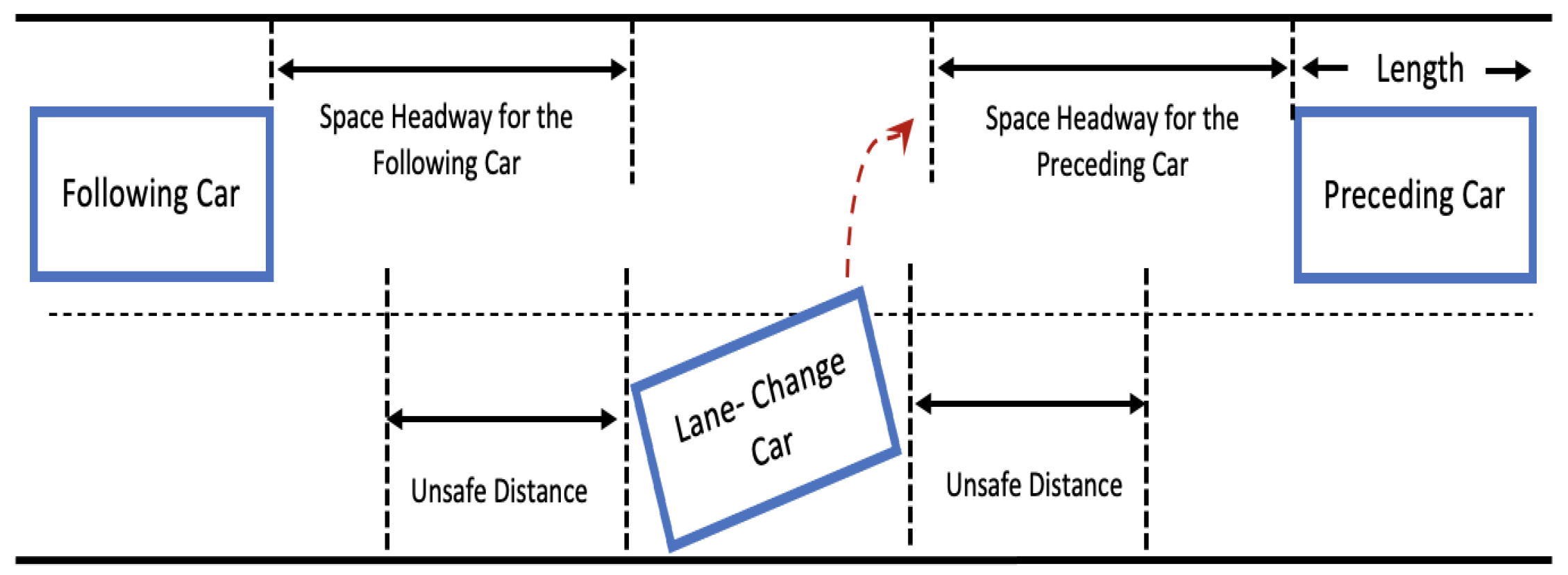
 - Lane Changing Models: Lane-changing algorithms are used to simulate the impact of vehicles on adjacent lanes as they change lanes. These algorithms take into account the speed and position of the preceding vehicle as well as the time when this action takes place [72]. The concept of the lane-changing algorithm can be simply described as follows. When the vehicle intends to change lanes, the model assesses the existing headway space to determine whether changing lanes is achievable. If it is, then the process happens. If not, then the vehicle remains in the current lane [73]. A simple illustration of the lane-changing decision of a vehicle is depicted in Figure 6. The model must meet certain criteria such that for a given adjacent lane, both the space headway for the following and preceding cars must be more than the unsafe distance, which can be computed as follows:Let and denote the following and preceding vehicle speeds, respectively, and b be the vehicle’s maximum deceleration. We refer to the actual vehicle following distance if the vehicle moved into the adjacent lane by d. Equation (9) is derived from Equations (7) and (8), which compute the smallest acceptable headway gap between each vehicle C and the minimum safe distance between the subject vehicle and the following vehicle [66,74].Figure 6. Basic lane-change model.

- Gap acceptance models: Gap-acceptance models are mainly used to determine the traffic conditions in adjacent lanes prior to a vehicle accessing the available space. They are used to estimate the amount of space and time required to cross a junction, enter a roundabout, or change lanes [75]. These two factors are dependent on the traffic conditions, such as the road characteristics, the speed, and the lengths of the following and preceding vehicles as well as the passive vehicle. The minimum safe distance between the subject vehicle and the following vehicle, which is also known as the critical gap, is a significant parameter affecting gap acceptance behavior. An important assumption that has to be addressed in the gap acceptance models is the headway distribution in the circulating flow to measure the road capacity [66,76]:where Y denotes the vehicle’s decision of whether or not to overtake the adjacent lane at a given time , is the available headway gap, and is the critical gap. The vehicle forces entry when the gap size is equally likely to be accepted ; otherwise, the vehicle rejects the observed gap and stays in the same lane [75].


5.2. Traffic Simulation Tools
- The Verkehr In Städten - SIMulationsmodell (VISSIM) is a commercial microscopic traffic simulation tool developed by Planning Transport Verkehr in Karlsruhe, Germany [77]. VISSIM is one of the common simulation tools used to simulate and evaluate traffic status and transportation control systems. It can simulate different elements such as buses, trucks, pedestrians, and bicycles. VISSIM uses the component object model (COM) interface, which enables users to create and deploy a custom tool in VISSIM using C++, Visual Basic, or Python [54]. The latest versions of VISSIM incorporate additional autonomous vehicle-related features (communication and cooperation among vehicles) and detailed behavior specifications. The aforementioned features will utilize cooperation in lane changing and advanced merging algorithms for enhanced traffic network scaling. In this simulator, smaller headways have been chosen to model the cooperation among vehicles. Other add-on features are the new means of mobility that have also been introduced within the VISSIM simulator, which include cooperative autonomous vehicles (CAVs) and mobility as a service (MAAS) [78]. VISSIM is a microscopic traffic simulator for behavior-based multi-purpose traffic flow simulation [79].
- Advanced Interactive Microscopic Simulator for Urban and Non-Urban Networks (AIMSUN) is a new simulation tool that was developed by J. Barcelo and J.L. Ferrer in 2005 [80]. It is a commercial simulation tool that is capable of simulating real-world traffic situations in an urban network in order to build and validate traffic structures, public transportation networks, and new transportation infrastructure [54]. AIMSUN is integrated with GETRAM, a simulation environment that includes different components: a traffic network editor (TEDI), a network database, a simulation module, and an application programming interface [81]. AIMSUN has developed AIMSUN LIVE, which integrates predictive-based systems that can provide real-time traffic prediction and management. In this aspect, AIMSUN LIVE can provide accurate real-time predictions of future traffic flow patterns that can be the outcome of a specific traffic management strategy. This is because AIMSUN LIVE leverages the combination of historical and real-time streaming data along with traffic congestion mitigation policies to provide accurate traffic forecasting. Subsequently, this can assist traffic control centers in utilizing the aforementioned traffic data to make real-time decisions about road network management [55].
- Multi-Agent Transport Simulation (MATSim) is another open-source simulation tool developed by the Polytechnic of Zurich that offers a range of tools for implementing very large simulation-based agents. In MATSIM, agents hold a list that simulates the daily routine of traffic in a large area. MATSIM adopts activity-based methods that are used to model travel demand. Since MATSIM is an agent-based simulator, these agents hold a list of actionable plans and choices which includes traditional traffic properties (e.g., travel routes and modes) and time schedules. In the MATSIM simulator, agents make their decisions according to the utilization of the integrated discrete choice models [82]. MATSIM mainly focuses on modeling individual vehicle behavior, which can be considered a drawback if we are interested in traffic behavior in general [54,83].
- Simulation of Urban MObility (SUMO) is an open-source simulation tool that was developed in 2001 by the Institute of Transportation Systems at the German Aerospace Centre. It is capable of simulating traffic at the microscopic level and simulates moving vehicles and accidents [84]. In this simulator, the vehicle width is fixed, and it does not take into account the different types of vehicles such as buses, light rail, heavy rail, and trucks [54,77]. SUMO is designed as an intermodal traffic-based simulator that includes public transportation, traffic road networks, and users such as pedestrians. SUMO simulators encompass a number of built-in features which include C2X communication among vehicles that are achieved through the integration of SUMO simulators with network simulators (such as OMNeT++ or ns-3), multi-modal traffic, and automated driving. Traffic management is also an additional add-on feature that can model vehicle detection loops and video detectors to manage and control traffic through traffic lights, monitoring vehicles’ behaviors and adjusting traffic parameters such as vehicles’ speed limits [58,85].
- CORridor SIMulation (CORSIM) [86] is known as one of the most widely used microscopic traffic simulator software programs worldwide. CORSIM is used in thousands of applications as a standard traffic simulation tool. CORSIM is equipped with reliable validation, continuous logic enhancement, solid verification, and calibration efforts. It can produce real-world traffic flow realistically and with high accuracy. All types of geometric conditions including complicated traffic scenarios can be handled virtually by CORSIM. Some of these conditions include the surfaces of streets that have different combinations of turning pockets and lanes, different types of on and off-ramps, and multi-lane freeway segments.
- Paramics addresses road networks with drivers and simulates the decisions, intentions, and subsequent actions of drivers when they move toward their destinations [87]. Depending on the characteristics of the basic network and the probability of encountering traffic congestion, drivers are considered to choose the possible route in the simulator. A set of decisions is prioritized by each driver throughout the network. These decisions include traffic speed and specific moments to change, cross, or merge into different traffic lanes. In the Paramics simulator, the network topology and travel demand drive the calibration. Flows of saturation and the proportion of lane usage are generated as outputs from the simulator to examine the road network’s performance. However, these parameters cannot be provided as input for calibration assistance. Although Paramics does not prescribe the effect of a traffic model, it can simulate and model the cause of action. This way, the simulator preserves the predictive power of the simulation process in subsequent changes in the model and tests the change in the traffic road network.
- The TRansportation ANalysis and SIMulation System (TRANSIMS) creates an integrated regional transportation system environment by employing advanced computational and analytical techniques [88]. The simulation environment includes a regional population of individual travelers. TRANSIMS simulates the activities and individual interactions of travelers and their plans for the transportation system. It also simulates and determines the environmental impact of these activities. TRANSIMS contains an interim operational capability (IOC) with numerous features, applicability, and readiness for each major module to complete different types of specific traffic case studies.
5.3. Summary of the Traffic Simulation Tools
- A major drawback of the exciting simulation tools is the inability to implement or integrate advanced Bayesian-based models or algorithms. They use the objective optimization algorithm to simulate traffic behavior based on different traffic parameters such as route choice and vehicle movement.
- Another issue that has gained the attention of the traffic simulation community is the CPU and memory performance. Adding a number of parameters to represent different aspects of the traffic simulation model such as traffic speed, the number of lanes, route length, and the width of the lane requires high usage of memory and the CPU, thus increasing the computation time.
- These traffic simulators embed sample events that we examine for their impact on the traffic status. These events are implemented as modules to represent limited events. These traffic simulators share similar events such as traffic acceleration events, traffic deceleration events, and traffic red signal events.

| Feature Simulator | MATSim | AIMSUN | VISSIM | SUMO | CORSIM | Paramics | TRANSIMS |
|---|---|---|---|---|---|---|---|
| Open Source | Yes | No | No | Yes | No | No | Yes |
| Visualization | 2D | 2D, 3D | 2D, 3D | 2D, 3D | 2D, 3D | 2D, 3D | 2D, 3D |
| Output | Text | Graphs | XML | XML | Text | Graphs | XML |
| Import Map | Yes | Yes | Yes | Yes | Yes | Yes | Yes |
| Programming Language | C++, Java | Python, C++ | C++, VB, Matlab, Python | C++, VB, Matlab, Python | Python, C++ | C++, VB, Matlab, Python | C++, VB, Matlab, Python |
| Flexibility in infrastructure Development | Limited | Flexible | Flexible | Flexible | Flexible | Flexible | Flexible |
| Coding | Easy | Difficult | Easy | Difficult | Difficult | Easy | Difficult |
| Objectives | Simulate traffic congestion level | Simulate vehicle counts, road occupancy, and traffic speed | Simulate and analyze traffic flow | Evaluate the traffic light system | Simulate traffic flow and traffic light system | Simulate traffic congestion level | Simulate and analyze traffic flow |
6. Conclusions
Author Contributions
Funding
Data Availability Statement
Conflicts of Interest
References
- Chao, W.; Quddus, M.; Ison, S. A spatio-temporal analysis of the impact of congestion on traffic safety on major roads in the UK. Transp. A Transp. Sci. 2013, 9, 124–148. [Google Scholar]
- Bachechi, C.; Po, L. Traffic analysis in a smart city. In Proceedings of the WI ’19: IEEE/WIC/ACM International Conference on Web Intelligence-Companion, Thessaloniki, Greece, 14–17 October 2019. [Google Scholar]
- Antonella, F.; Sacone, S.; Siri, S. Freeway Traffic Modeling and Control; Springer: Berlin/Heidelberg, Germany, 2018. [Google Scholar]
- Xiaokun, W.; Kockelman, K.M. Forecasting network data: Spatial interpolation of traffic counts from Texas data. Transp. Res. Rec. 2015, 2105, 100–108. [Google Scholar]
- Nectaria, T.; Jensen, C.S. Conceptual data modeling for spatiotemporal applications. GeoInformatica 1999, 3, 245–268. [Google Scholar]
- Algers, S.; Bernauer, E.; Boero, M.; Breheret, L.; Taranto, C.; Fox, K. A Review of Micro-Simulation Models, SMARTEST: Simulation Modeling Applied to Transport European Scheme Tests; Institute for Transport Studies, University of Leeds: Leeds, UK, 1996; pp. 100–108. [Google Scholar]
- Ejercito Paolo, M.; Kristine Gayle, E.; Nebrija, R.P.F.; Lara-Figueroa, L.L. Traffic simulation software review. In Proceedings of the 2017 8th International Conference on Information, Intelligence, Systems & Applications (IISA), Larnaca, Cyprus, 28–30 August 2017. [Google Scholar]
- TomTom. Traffic Congestion Ranking|TomTom Traffic Index. Available online: https://tomtom.com/en-gb/traffic-index/ranking/ (accessed on 2 March 2022).
- Government of Canada. Canadian Motor Vehicle Traffic Collision Statistics: 2018. Available online: https://tc.canada.ca/en/road-transportation/statistics-data/canadian-motor-vehicle-traffic-collision-statistics-2018 (accessed on 1 March 2022).
- Box George, E.P.; Tiao George, C. Bayesian Inference in Statistical Analysis; John Wiley and Sons: Hoboken, NJ, USA, 2011; Volume 40. [Google Scholar]
- Eleni, V.; Karlaftis, M.G.; Golias, J.C. Short-term traffic forecasting: Where we are and where we’re going. Transp. Res. Part C Emerg. Technol. 2014, 43, 3–19. [Google Scholar]
- Xiaolei, M.; Dai, Z.; He, Z.; Ma, J.; Wang, Y.; Wang, Y. Learning traffic as images: A deep convolutional neural network for large-scale transportation network speed prediction. Sensors 2017, 17, 818. [Google Scholar]
- Afshin, A.; Rajabioun, T.; Ioannou, P. Traffic flow prediction for road transportation networks with limited traffic data. IEEE Trans. Intell. Transp. Syst. 2014, 16, 653–662. [Google Scholar]
- Yisheng, L.; Duan, Y.; Kang, W.; Li, Z.; Wang, F.-Y. Traffic flow prediction with big data: A deep learning approach. IEEE Trans. Intell. Transp. Syst. 2014, 16, 865–873. [Google Scholar]
- Zhanguo, S.; Guo, Y.; Wu, Y.; Ma, J. Short-term traffic speed prediction under different data collection time intervals using a SARIMA-SDGM hybrid prediction model. PloS ONE 2019, 14, e0218626. [Google Scholar]
- Ibai, L.; Ser, J.D.; Velez, M.; Vlahogianni, E. Road traffic forecasting: Recent advances and new challenges. IEEE Intell. Transp. Syst. Mag. 2018, 10, 93–109. [Google Scholar]
- Reisen Valdério, A.; Zamprogno, B.; Palma, W.; Arteche, J. A semiparametric approach to estimate two seasonal fractional parameters in the SARFIMA model. Math. Comput. Simul. 2014, 98, 1–17. [Google Scholar] [CrossRef]
- Raikwar Aditya, R.; Sadawarte, R.R.; More, R.G.; Gunjal, R.S.; Mahalle, P.N.; Railkar, P.N. Long-term and short-term traffic forecasting using holt-winters method: A comparability approach with comparable data in multiple seasons. Int. J. Synth. Emot. (IJSE) 2017, 8, 38–50. [Google Scholar] [CrossRef]
- Antti, S.; Hao, J.; Reyhani, N.; Ji, Y.; Lendasse, A. Methodology for long-term prediction of time series. Neurocomputing 2007, 70, 2861–2869. [Google Scholar]
- Gregorio, G.; Rossi, R.; Gastaldi, M.; Caprini, A. Data mining methods for traffic monitoring data analysis: A case study. Procedia-Soc. Behav. Sci. 2011, 20, 455–464. [Google Scholar]
- Yi, Y.; Shang, P. Forecasting traffic time series with multivariate predicting method. Applied Math. Comput. 2016, 3, 266–278. [Google Scholar]
- Qianlong, W.; Guo, Y.; Yu, L.; Li, P. Earthquake prediction based on spatio-temporal data mining: An LSTM network approach. IEEE Trans. Emerg. Top. Comput. 2017, 8, 148–158. [Google Scholar]
- Brent, S.; Kockelman Kara, M. Spatial prediction of traffic levels in unmeasured locations: Applications of universal Kriging and geographically weighted regression. J. Transp. Geogr. 2013, 29, 24–32. [Google Scholar]
- John, O.K.; Vaci, L.; Mihaylova, L.S. Traffic estimation for large urban road network with high missing data ratio. Sensors 2019, 19, 2813. [Google Scholar]
- Matthew, H.; Amer, H.M.; Mihaylova, L. Traffic state estimation via a particle filter over a reduced measurement space. In Proceedings of the 2017 20th International Conference on Information Fusion (Fusion), Xi’an, China, 10–13 July 2017; pp. 1–8. [Google Scholar]
- Matthew, H.; Amer, H.M.; Mihaylova, L. Traffic volume prediction with segment-based regression Kriging and its implementation in assessing the impact of heavy vehicles. IEEE Trans. Intell. Transp. Syst. 2018, 20, 232–243. [Google Scholar]
- Haixiang, Z.; Yang, Y.; Qingquan, L.; Go, Y.A. An improved distance metric for the interpolation of link-based traffic data using Kriging: A case study of a large-scale urban road network. Int. J. Geogr. Inf. Sci. 2012, 26, 667–689. [Google Scholar]
- Hackney Jeremy, K.; Michael, B.; Sumit, B.; Axhausen Kay, W. Predicting road system speeds using spatial structure variables and network characteristics. J. Geogr. Syst. 2007, 9, 397–417. [Google Scholar] [CrossRef]
- Hidetoshi, M. A Study of Travel Time Prediction Using Universal Kriging; Springer: Berlin/Heidelberg, Germany, 2010; pp. 257–270. [Google Scholar]
- John, S. Nested sampling for general Bayesian computation. Bayesian Anal. 2006, 1, 2833–2859. [Google Scholar]
- Lee Peter, M. Bayesian Statistics; Oxford University Press: London, UK, 1989. [Google Scholar]
- Daziano Ricardo, A.; Luis, M.-M.; Shahram, H. Computational Bayesian statistics in transportation modeling: From road safety analysis to discrete choice. Transp. Rev. 2013, 33, 570–592. [Google Scholar] [CrossRef]
- Subhadeep, M.; Fletcher, D. Generalized empirical Bayes modeling via frequentist goodness of fit. Sci. Rep. 2018, 8, 1–15. [Google Scholar]
- Lai, Z.; Tarek, S. Bayesian hierarchical modeling of traffic conflict extremes for crash estimation: A non-stationary peak over threshold approach. Anal. Methods Accid. Res. 2019, 24, 100–106. [Google Scholar]
- Faustino, P.; Gómez-Déniz, E.; Sarabia, J.M. Modeling road accident blackspots data with the discrete generalized Pareto distribution. Accid. Anal. Prev. 2014, 71, 38–49. [Google Scholar]
- Kumar, M.; Raghuwanshi, N.S.; Singh, R. Artificial neural networks approach in evapotranspiration modeling: A review. Irrig. Sci. 2011, 29, 11–25. [Google Scholar] [CrossRef]
- Mohamed Zahraa, E. Using the artificial neural networks for prediction and validating solar radiation. J. Egypt. Math. Soc. 2019, 27, 1–13. [Google Scholar] [CrossRef]
- Gregorio, G.; Riccardo, R.; Massimiliano, G.; Armando, C. Data mining methods for traffic monitoring data analysis: A case study. Procedia-Soc. Behav. Sci. 2011, 29, 455–464. [Google Scholar]
- Chen, W.; Guo, F.; Wang, F.-Y. A survey of traffic data visualization. IEEE Trans. Intell. Transp. Syst. 2015, 16, 2970–2984. [Google Scholar] [CrossRef]
- Gültekin, Ç.B.; Sari, M.; Borat, O. A neural network based traffic-flow prediction model. Math. Comput. Appl. 2010, 15, 269–278. [Google Scholar]
- Romi, S.; Jonathan, A.; Maria, C. Spatial analysis of road crash frequency using Bayesian models with Integrated Nested Laplace Approximation (INLA). J. Transp. Saf. Secur. 2021, 13, 1240–1262. [Google Scholar]
- Cynthia, T.; Deirdre, M.; Jonathan, A. Freeway traffic data prediction using neural networks. In Proceedings of the Pacific Rim TransTech Conference, 1995 Vehicle Navigation and Information Systems Conference Proceedings, 6th International VNIS. A Ride into the Future, Seattle, WA, USA, 30 July–2 August 1995; IEEE: Piscataway, NJ, USA, 1995; pp. 225–230. [Google Scholar]
- Cheng, C.A.; Boots, B. Variational inference for Gaussian process models with linear complexity. arXiv 2017, arXiv:1711.10127. [Google Scholar]
- Somnath, C. Spatio-Temporal Modeling of Traffic Risk Mapping on Urban Road Networks. Master’s Thesis, Jaume I University, Castelló, Spain, February 2020. [Google Scholar]
- Dawkins, L.C.; Williamson, D.B.; Mengersen, K.L.; Morawska, L.; Jayaratne, R.; Shaddick, G. Where is the clean Air? A bayesian decision framework for personalised cyclist route selection using R-INLA. Bayesian Anal. 2021, 16, 61–91. [Google Scholar] [CrossRef]
- Broemeling Lyle, D. Bayesian methods for medical test accuracy. Diagnostics 2011, 1, 1. [Google Scholar] [CrossRef] [PubMed]
- Spiegelhalter, D.J.; Best, N.G.; Carlin, B.P.; Van Der Linde, A. Bayesian measures of model complexity and fit. J. R. Stat. Soc. Ser. B (Stat. Methodol.) 2002, 64, 583–639. [Google Scholar] [CrossRef]
- Daniels Michael, J.; Hogan Joseph, W. Missing Data in Longitudinal Studies: Strategies for Bayesian Modeling and Sensitivity Analysis; CRC Press: Boca Raton, FL, USA, 2008. [Google Scholar]
- Van De Schoot, R.; Broere, J.J.; Perryck, K.H.; Zondervan-Zwijnenburg, M.; Van Loey, N.E. Analyzing small data sets using Bayesian estimation: The case of posttraumatic stress symptoms following mechanical ventilation in burn survivors. Eur. J. Psychotraumatology 2015, 6, 25216. [Google Scholar] [CrossRef]
- Gary, C.; Dan, L. When optimal choices feel wrong: A laboratory study of Bayesian updating, complexity, and affect. Am. Econ. Rev. 2005, 95, 1300–1309. [Google Scholar]
- Khaz’ali, A.R.; Emamjomeh, A.; Andayesh, M. An accuracy comparison between artificial neural network and some conventional empirical relationships in estimation of relative permeability. Pet. Sci. Technol. 2011, 29, 1603–1614. [Google Scholar] [CrossRef]
- Alireza, K.; Nayyara, S. Multi-scale high-speed network traffic prediction using combination of neural networks. In Proceedings of the International Joint Conference on Neural Networks, Portland, OR, USA, 20–24 July 2003; pp. 1071–1075. [Google Scholar]
- Alfréd, C.; Viharos, Z.J.; Kis, K.B.; Tettamanti, T.; Varga, I. Traffic speed prediction method for urban networks—An ANN approach. In Proceedings of the 2015 International Conference on Models and Technologies for Intelligent Transportation Systems (MT-ITS), Budapest, Hungary, 3–5 June 2015. [Google Scholar]
- Nesrine, G.; Sabeur, E.; Saber, D.; Ben, S.L. A survey of simulation platforms for the assessment of public transport control systems. In Proceedings of the 2014 International Conference on Advanced Logistics and Transport (ICALT), Tunis, Tunisia, 1–3 May 2014. [Google Scholar]
- Djukic, T.; van Lint, H.; Casas, J. An open, sustainable, ubiquitous data and service ecosystem for efficient, effective, safe, resilient mobility in metropolitan areas. H2020-ICT 2015. [Google Scholar] [CrossRef]
- US Department of Transportation. Types of Traffic Analysis Tools. Available online: https://ops.fhwa.dot.gov/trafficanalysistools/typetools.htm (accessed on 11 March 2022).
- David, W.; Sewall, J.; Li, W.; Lin, M.C. Virtualized traffic at metropolitan scales. Front. Robot. AI 2015, 2, 11. [Google Scholar]
- Saidallah, M.; Fergougui, A.E.; Elalaoui, A.E. A comparative study of urban road traffic simulators. MATEC Web Conf. 2016, 81, 05002. [Google Scholar] [CrossRef]
- Sohel, M.S.M.; Ferreira, L.; Hoque, M.S.; Tavassoli, A. Micro-simulation modeling for traffic safety: A review and potential application to heterogeneous traffic environment. IATSS Res. 2019, 43, 27–36. [Google Scholar]
- Sokolowski John, A.; Banks Catherine, M. Principles of Modeling and Simulation: A Multidisciplinary Approach; John Wiley & Sons: Hoboken, NJ, USA, 2011. [Google Scholar]
- Zhang, Y.; Owen Larry, E.; Clark James, E. Multiregime approach for microscopic traffic simulation. Transp. Res. Rec. 1998, 1644, 103–114. [Google Scholar] [CrossRef]
- Miller, J.; Horowitz, E. FreeSim—A free real time freeway traffic simulator. In Proceedings of the 2007 IEEE Intelligent Transportation Systems Conference, Seattle, WA, USA, 30 September–3 October 2007; pp. 18–23. [Google Scholar]
- Lindorfer, M.; Backfrieder, C.; Mecklenbräuker, C.F.; Ostermayer, G. Modeling Isolated Traffic Control Strategies in TraffSim. In Proceedings of the UKSim-AMSS 19th International Conference on Computer modeling & Simulation (UKSim), Cambridge, UK, 5–7 April 2017; pp. 143–148. [Google Scholar]
- Cai, P.; Lee, Y.; Luo, Y.; Hsu, D. SUMMIT: A Simulator for Urban Driving in Massive Mixed Traffic. In Proceedings of the IEEE International Conference on Robotics and Automation (ICRA), Virtually, 31 May–31 August 2020; pp. 4023–4029. [Google Scholar]
- Sorenson, D.K.; Collins, J. Practical Applications Of Traffic Simulation Using SifTraffic. Presented at the Compendium of Papers, Institute of Transportation Engineers 2000, District 6 Annual Meeting, San Diego, CA, USA, 24–28 June 2000; Available online: https://trid.trb.org/view/671329 (accessed on 30 July 2021).
- Usman, A.H.; Huang, Y.; Lu, P. A review of car-following models and modeling tools for human and autonomous-ready driving behaviors in micro-simulation. Smart Cities 2021, 4, 314–335. [Google Scholar]
- Rothery, R.W. Car Following Models. 1992. Available online: https://ocw.mit.edu/courses/1-225j-transportation-flow-systems-fall-2002/a884475721d0645b8ce2ee8640976caf_carfollowinga.pdf (accessed on 11 March 2022).
- Janson, O.J.; Tapani, A. Comparison of Car-Following Models; Swedish National Road and Transport Research Institute: Linkö ping, Sweden, 2004; Volume 960. [Google Scholar]
- Aycin, M.F.; Benekohal, R.F. Comparison of car-following models for simulation. Transp. Res. Rec. 1999, 1678, 1116–1127. [Google Scholar] [CrossRef]
- Haiyang, Y.; Jiang, R.; He, Z.; Zheng, Z.; Li, L.; Liu, R.; Chen, X. Automated vehicle-involved traffic flow studies: A survey of assumptions, models, speculations, and perspectives. Transp. Res. Part C Emerg. Technol. 2021, 127, 1–127. [Google Scholar]
- Yang, D.; Zhu, L.; Liu, Y.; Wu, D.; Ran, B. A novel car-following control model combining machine learning and kinematics models for automated vehicles. IEEE Trans. Intell. Transp. Syst. 2018, 20, 1991–2000. [Google Scholar]
- Sara, M.; Sarvi, M.; Rose, G. Lane changing models: A critical review. Transp. Lett. 2010, 2, 157–173. [Google Scholar]
- Gipps Peter, G. A model for the structure of lane-changing decisions. Transp. Res. Part Methodol. 1986, 20, 403–414. [Google Scholar] [CrossRef]
- Mizanur, R.; Chowdhury, M.; Xie, Y.; He, Y. Review of microscopic lane-changing models and future research opportunities. IEEE Trans. Intell. Transp. Syst. 2013, 14, 1942–1956. [Google Scholar]
- Rahmi, A. A Review Of Gap-Acceptance Capacity Models. In Proceedings of the Conference of Australian Institutes of Transport Research (Caitr), Adelaide, Australia, 5–7 December 2017. [Google Scholar]
- Ahmed, K.; Ben-Akiva, M.; Koutsopoulos, H.; Mishalani, R. Models of freeway lane changing and gap acceptance behavior. Transp. Traffic Theory 1996, 13, 501–515. [Google Scholar]
- Kotusevski, G.; Hawick, K.A. A review of traffic simulation software. Res. Lett. Inf. Math. Sci. 2009, 13, 35–54. [Google Scholar]
- PTV Group. PTV Vissim is the World’s Most Advanced and Flexible Traffic Simulation Software. Available online: https://www.ptvgroup.com/en/solutions/products/ptv-vissim/ (accessed on 11 March 2022).
- Fellendorf, M.; Vortisch, P. Microscopic traffic flow simulator VISSIM. In Fundamentals of Traffic Simulation; Barceló, J., Ed.; Springer: New York, NY, USA, 2010; pp. 63–93. [Google Scholar]
- Jordi, C.; L, F.J.; David, G.; Josep, P.; Alex, T. Traffic Simulation with Aimsun; Springer: Berlin/Heidelberg, Germany, 2010. [Google Scholar]
- Rehmat, U.M.; Shehzad, K.K.; Hussain, K.Z.; Ahmad, K.M.; Nasru, M.; Nawaz, K.A. Vehicular Traffic Simulation Software: A Systematic Comparative Analysis. Pak. J. Eng. Technol. 2021, 4, 103–114. [Google Scholar]
- Johannes, N.; Powers, S.T.; Urquhart, N.; Farrenkopf, T.; Guckert, M. An overview of agent-based traffic simulators. Transp. Res. Interdiscip. Perspect. 2021, 12, 100486. [Google Scholar]
- Andreas, H.; Kai, N.; Axhausen Kay, W. The Multi-Agent Transport Simulation MATSim; Ubiquity Press: London, UK, 2016. [Google Scholar]
- Alvarez, L.P.; Behrisch, M.; Bieker-Walz, L.; Erdmann, J.; Flötteröd, Y.; Hilbrich, R.; Lücken, L.; Rummel, J.; Wagner, P.; Wießner, E. Microscopic Traffic Simulation Using sumo. In Proceedings of the 2018 21st International Conference on Intelligent Transportation Systems (ITSC), Maui, HI, USA, 4–7 November 2018; IEEE: Piscataway, NJ, USA, 2018; pp. 2575–2582. [Google Scholar]
- SUMO. Simulation of Urban Mobility. Available online: https://www.eclipse.org/sumo/ (accessed on 11 March 2022).
- Owen, L.E.; Zhang, Y.; Rao, L.; McHale, G. Traffic flow simulation using CORSIM. In Proceedings of the 2000 Winter Simulation Conference Proceedings (Cat. No.00CH37165), Orlando, FL, USA, 10–13 December 2000; Volume 2, pp. 1143–1147. [Google Scholar]
- Sykes, P. Traffic Simulation with Paramics. In Fundamentals of Traffic Simulation; Barceló, J., Ed.; Springer: New York, NY, USA, 2010; pp. 131–171. [Google Scholar]
- Smith, L.; Beckman, R.; Baggerly, K. TRANSIMS: Transportation Analysis and Simulation System; Los Alamos National Lab. (LANL): Los Alamos, NM, USA, 1995. [Google Scholar]


| Bayesian Inferences | ST-Kriging | ANNs | |
|---|---|---|---|
| Computational Complexity | NP-hard. [41] | . | or for training a single epoch [42]. |
| Performance Evaluation | Provides a posterior probability distribution with confidence interval. | Ensure linear unbiased predictors. | Epoch with the lowest sum of squared error. |
| Weaknesses | Very computationally intensive due to choosing the proper prior distribution. |
| Requires intensive data training, and this might lead to an overfitting problem. |
| Strengths |
|
|
|
| Overcoming the Limitation | Use uninformative prior to reducing the computational time, but it can affect the prediction accuracy negatively. | Remove observations that include missing values. |
|
Publisher’s Note: MDPI stays neutral with regard to jurisdictional claims in published maps and institutional affiliations. |
© 2022 by the authors. Licensee MDPI, Basel, Switzerland. This article is an open access article distributed under the terms and conditions of the Creative Commons Attribution (CC BY) license (https://creativecommons.org/licenses/by/4.0/).
Share and Cite
Alghamdi, T.; Mostafi, S.; Abdelkader, G.; Elgazzar, K. A Comparative Study on Traffic Modeling Techniques for Predicting and Simulating Traffic Behavior. Future Internet 2022, 14, 294. https://doi.org/10.3390/fi14100294
Alghamdi T, Mostafi S, Abdelkader G, Elgazzar K. A Comparative Study on Traffic Modeling Techniques for Predicting and Simulating Traffic Behavior. Future Internet. 2022; 14(10):294. https://doi.org/10.3390/fi14100294
Chicago/Turabian StyleAlghamdi, Taghreed, Sifatul Mostafi, Ghadeer Abdelkader, and Khalid Elgazzar. 2022. "A Comparative Study on Traffic Modeling Techniques for Predicting and Simulating Traffic Behavior" Future Internet 14, no. 10: 294. https://doi.org/10.3390/fi14100294
APA StyleAlghamdi, T., Mostafi, S., Abdelkader, G., & Elgazzar, K. (2022). A Comparative Study on Traffic Modeling Techniques for Predicting and Simulating Traffic Behavior. Future Internet, 14(10), 294. https://doi.org/10.3390/fi14100294