Spiking Neural Network-Based Near-Sensor Computing for Damage Detection in Structural Health Monitoring

Abstract

In this work, we present an innovative approach for damage detection of infrastructures on-edge devices, exploiting a brain-inspired algorithm. The proposed solution exploits recurrent spiking neural networks (LSNNs), which are emerging for their theoretical energy efficiency and compactness, to recognise damage conditions by processing data from low-cost accelerometers (MEMS) directly on the sensor node. We focus on designing an efficient coding of MEMS data to optimise SNN execution on a low-power microcontroller. We characterised and profiled LSNN performance and energy consumption on a hardware prototype sensor node equipped with an STM32 embedded microcontroller and a digital MEMS accelerometer. We used a hardware-in-the-loop environment with virtual sensors generating data on an SPI interface connected to the physical microcontroller to evaluate the system with a data stream from a real viaduct. We exploited this environment also to study the impact of different on-sensor encoding techniques, mimicking a bio-inspired sensor able to generate events instead of accelerations. Obtained results show that the proposed optimised embedded LSNN (eLSNN), when using a spike-based input encoding technique, achieves 54% lower execution time with respect to a naive LSNN algorithm implementation present in the state-of-the-art. The optimised eLSNN requires around 47 kCycles, which is comparable with the data transfer cost from the SPI interface. However, the spike-based encoding technique requires considerably larger input vectors to get the same classification accuracy, resulting in a longer pre-processing and sensor access time. Overall the event-based encoding techniques leads to a longer execution time (1.49×) but similar energy consumption. Moving this coding on the sensor can remove this limitation leading to an overall more energy-efficient monitoring system.

1. Introduction

The application of distributed sensors to pervasive monitoring of physical processes is one of the most critical and relevant domains. In particular, Structural Health Monitoring (SHM) is a key deployment scenario, where ensuring the safety of infrastructures such as buildings and bridges can be, in principle, achieved by deploying low-cost sensors to detect structural variations due to damages. The convergence of Artificial Intelligence (AI) to Internet-of-Things (IoT) and edge computing in this domain can help approach these challenges. In this context, executing AI detection algorithms directly on the IoT sensor nodes potentially reduces data transmission overheads and improves response time. A review of recent embedded AI approaches to detection in SHM can be found in [1]. Due to the low-cost, low-power and increasing accuracy of MEMS accelerometers, their application to distributed SHM is becoming popular.

Signal compression techniques on-edge have also been proposed to compress MEMS data gathered from several nodes and send them to the cloud storage and analytic facility [2]. Still, on MEMS data, on-sensor modal estimation was proposed by implementing procedures to detect relevant peaks in the acquired signal spectrum [3].

Optimized machine learning algorithms on-edge have been recently proposed to increase the intelligence of distributed detection for SHM. Considering the availability of code and libraries to implement machine learning algorithms on low-power microcontrollers [4,5], it is a viable solution to execute detection algorithms on-edge and on-sensor. In this context, hazard monitoring based on an array of event-triggered single-channel micro-seismic sensors with advanced signal processing is proposed, exploiting a Convolutional Neural Network (CNN) implemented on a low-power microcontroller, and can be found in [6].

Applied to anomaly detection on a highway bridge, in [7] a compression technique to identify anomalies in the structure using a semi-supervised approach is proposed using either a fully connected or a convolutional autoencoder implemented on the sensor node. In the present work we provide an alternative solution applied to the same case study using a supervised algorithm for near-sensor anomaly detection based on Spiking Neural Networks (SNNs). SNNs gained interest in the research community in various application domains, including SHM, because of their brain-inspired, event-based nature, which potentially allows reduced energy requirement compared to traditional ANN [8,9,10,11,12]. While Artificial Neural Networks (ANNs) have been successfully applied to SHM [1,13,14,15,16], SNNs are of increasing interest in this field because of their theoretical greater information processing efficiency achieved by exploiting a sparse computation approach. In [17] a feed forward SNN has been applied to low-cost, MEMS-based inspection of damaged buildings.

However, the state-of-art in SNN applications to SHM misses a real implementation of a data processing pipeline with the execution of SNN directly on the sensor node. Moreover, embedded machine learning libraries currently lack efficient SNN implementations.

In the context of SNN, when time-series data from sensors are concerned, recurrent neural networks have shown to be effective [18]. For this reason, instead of more simple feed-forward architectures, we investigate recurrent SNNs for SHM data processing. In particular we consider a state-of-art recurrent implementation of SNN called LSNN (long short-term SNN) introduced in [19] because of its interesting signal processing features and learning effectiveness. Moreover, a relevant aspect to be explored is the encoding of the input signal, which impacts subsequent computation steps and associated energy consumption. In particular, SNNs have been used with event-based input such as pixel variations from Dynamic Vision Sensor (DVS) cameras [20], but they can also effectively process “continuous” data streams in speech recognition applications [19]. However, in the context of SHM in general, which encoding is the best suited for anomaly detection task has not been studied so far.

This work presents the design, implementation, and characterisation of an LSNN on a low-power sensor node equipped with a commercial microcontroller and an MEMS accelerometer. The LSNN has been evaluated using real data from a highway viaduct, for which it was able to detect structural variations associated with a degraded condition. To the best of our knowledge, this is the first implementation of an LSNN on a low-power microcontroller that we integrated into a complete SNN-based near-sensor computing system. We designed and compared different input data encoding schemes in terms of performance and energy. We designed an optimised LSNN version for microcontroller targets, and we characterised its performance and energy consumption on silicon, including the overhead of data transfer from the MEMS sensor and the coding. Thanks to our hardware-in-the-loop measurement set-up, we were also able to emulate the behaviour of a smart sensor able to send spikes directly instead of acceleration values.

We compare with an alternative semi-supervised edge anomaly detection applied to the same dataset [7]. Authors of [7] show that the anomaly detection of the faulty and normal condition requires a complex pipeline. It consists of: (i) A filtering step; (ii) an anomaly detector; (iii) a final smoothing post-processing. They either propose principal component analysis compression and decompression or a fully connected autoencoder to implement the anomaly detector. The autoencoder features a single hidden layer of 32 neurons, an input layer with 500 samples, and an output layer with 500 neurons. Both these algorithms show a complexity of $500\times 32\times 2$ (32,000) multiply-and-accumulate operations. The neurons, intended as the application in the hidden and output layers of a non-linear function like sigmoid or RELU are 532 (hidden plus output neurons). Instead, the number of MAC operations is due to the number of connections. In this way, we have 500 × 32 MAC for the input-hidden layer and 32 × 500 MAC for the hidden-output layer, for a total of 500 × 32 × 2 MAC. We show that we can achieve similar accuracy results with considerably fewer computational resource; to solve the same detection problem, the proposed solution uses 15,750 sums and 750 multiplications.

While the two algorithms are not directly comparable because of the different ML approaches, the comparison against the reference testifies that the proposed solution is effective in solving the same detection problem. The contribution of this paper can be summarized as follows:

• We studied the computational requirements and complexity of the LSNN, and we provide an implementation on a low-power microcontroller-based sensor node.
• We designed and implemented an optimized LSNN version for performance constrained architectures, and we compared a continuous versus event-based input encoding.
• We evaluated the benefits of the proposed optimizations both theoretically and on real hardware, and we explored accuracy versus energy and performance trade-offs, including the cost of sensor data transfer.
• We demonstrate that LSNNs can be effectively executed near the MEMS sensor with a few tens of K cycles (comparable with data transfer cost) and deliver MCC levels higher than 0.75 (corresponding to almost 90% accuracy) using data from a real case study of damage detection in SHM.

The rest of this paper is organized as follows. Section 2 presents some background on SHM and LSNN. Section 3 presents the LSNN architecture, training and input coding methods. Section 4 explains the introduced optimizations. Section 5 reports the experimental test-bed and results, and Section 6 concludes the work.

2. Background

This section describes the SHM problem and the reference SoA monitoring system composed of sensor nodes, edge-node, and cloud architecture. We then give some background about Spiking Neural Networks and their recurrent LSNN counterparts, input coding strategy, and the training algorithm adopted. Finally, the sensor board and microcontroller used for measurements are introduced.

As described earlier, the manuscript focuses on the feasibility analysis of using a brain-inspired algorithm on the sensor-node MicroController Unit (MCU) and its implementation trade-offs. To experimentally validate this approach in Section 5 we describe the experimental setup consisting of a hardware-in-the-loop (HIL) approach.

2.1. Bridge Structure & SHM Framework

The structure under study is a highway viaduct (A32 Torino-Bardonecchia-S.S.335) built with eighteen sections, each one supported by two pairs of concrete pillars situated at their two ends. We focus on a single section instrumented for data analysis before a scheduled maintenance intervention in this work. Maintenance was necessary for the strengthening of the viaduct structure.

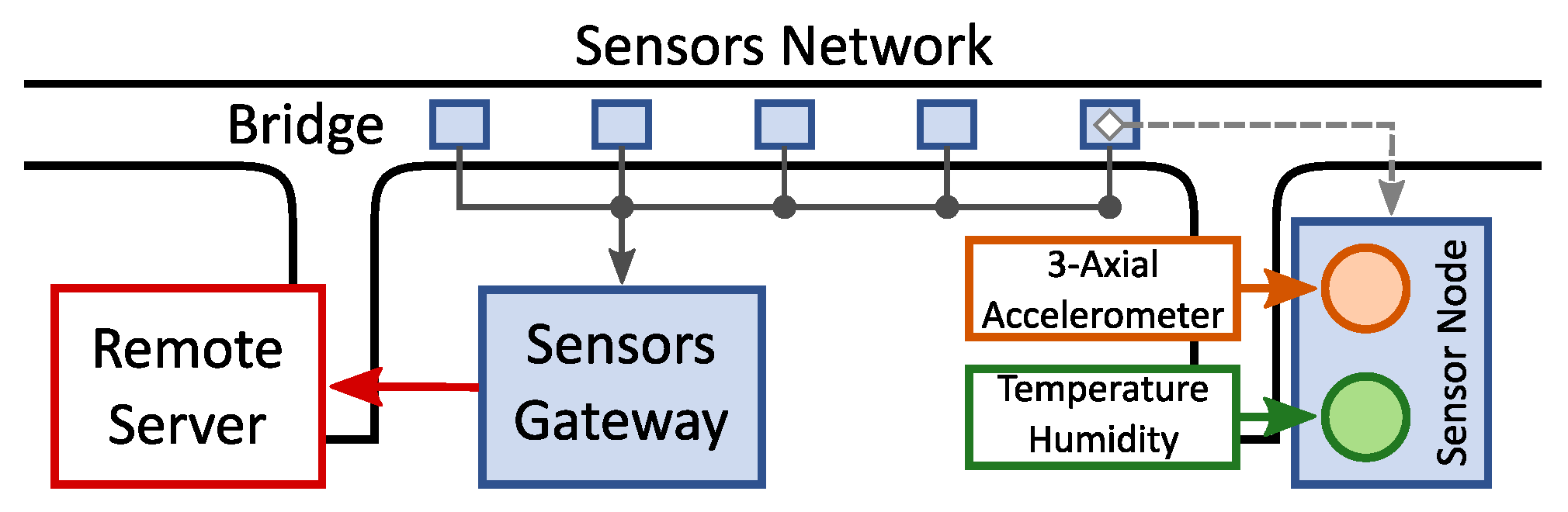
The acquisition framework is described in Figure 1. The system contains five identical sensor nodes. Each one features an STM32F4 microcontroller (MCU) and samples three-axis accelerations and temperature data, and stores them in the cloud through a 4G-connected Raspberry Pi3 gateway.

The five nodes are connected through CAN-BUS to the gateway. Note that the acquisition system only collects the data without any local edge-side signal processing. In this basic configuration, data analysis is executed on the cloud. The accelerometer samples the data with a frequency of 25.6 kHz to avoid aliasing. Subsequently, the data is subsampled to have a final output frequency ($f_s$) of 100 Hz.

The cloud part is composed of a data-ingestion job, which receives and store data from the gateway, and periodically scheduled analysis tasks to monitor the health status of the bridge [2].

The MCU is an ARM 32-bit Cortex-M4 running at 168 MHz, with 192 kB of SRAM and 1 MB of Flash memory, popular in different edge applications for its low power consumption. Further, the MCU features a floating-point unit and a digital signal processing (DSP) library. The gateway is a standard Raspberry Pi 3 module B [21] (RPi3). It includes a Broadcom BCM2837 SoC, with 64 bit 4-core Cortex-A53 running at 1.2 GHz and 1 GB of DDR2 RAM. The gateway runs an Ubuntu operating system, easing the scheduling of communication tasks through common python interfaces (e.g., an MQTT broker [22]). The cloud system is divided into a storage section and a computing node allocated on the IBM cloud service.

In this work, we propose to replace cloud processing with a brain-inspired near-sensor anomaly detection algorithm directly computed on the microcontroller (MCU) on the sensor node board. We will show that the proposed algorithm can identify the normal and faulty bridge conditions, avoiding the RAW data transmission to the cloud.

2.2. Structural Health Monitoring Data

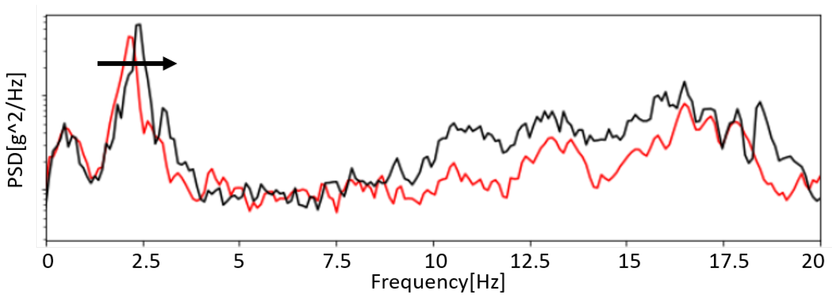
SHM frameworks usually process acceleration data for monitoring structures’ health status [23]. The datasets used in the study contain 3-axial accelerations data acquired with the previously described framework. As mentioned above, the viaduct underwent a technical intervention to strengthen its structure, with a corresponding change in the natural frequencies of a bridge. Figure 2 shows how the power spectrum density, averaged over 6 h, is modified before and after the intervention.

Given these data’s uniqueness, we use them as a proxy of an aged viaduct compared to a healthy one. In particular, in this work, we consider the signals collected after the intervention as the normal data produced by a healthy viaduct. Analogously, the data gathered before the maintenance intervention are considered “anomalies” since they are sampled on a damaged and aged bridge. While the data do not represent the whole history of the viaduct, to the best of our knowledge, it is the only dataset containing vibrations from the viaduct during two different structural phases of the building.

2.3. Spiking Neural Networks

This paper proposes to study a Spiking Neural Network Model to solve the SHM supervised anomaly detection problem directly on the sensor’s node MCU. The SNN model is a brain-inspired (so-called third-generation) type of neural network. They have a greater computational capacity as the single neuron is modelled with a much more complex dynamic than the neurons present in traditional Artificial Neural Networks (ANNs). This means that SNNs can solve the same tasks as ANNs with fewer neurons [8]. Moreover, their hardware implementation on neuromorphic architectures and accelerators can lead to greater energy efficiency in data management and computation [24,25,26,27,28]. In this work, we do not consider neuromorphic implementation because the objective is to work with low-cost commercial MCUs, for which SNN porting is not available.

In particular, we consider a recurrent type of SNN called LSNN (Long Short-Term SNN) because they are suitable to process temporal data streams like their artificial counterparts (e.g., LSTMs). While SNN has already attracted attention for SHM applications, so far, literature papers have focused on simple feed-forward SNN, which are less powerful and do not exploit the potential of SNN, nor do they impose training challenges [17].

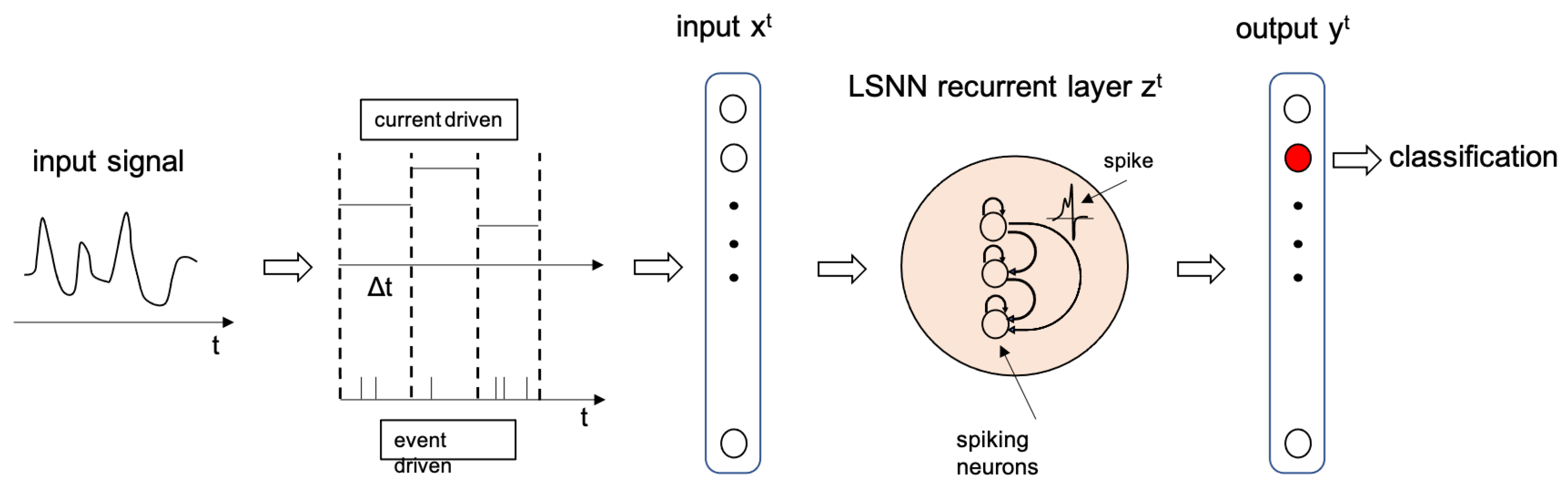
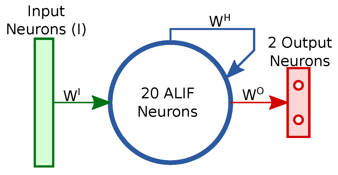
The recurrent LSNN structure is depicted in Figure 3, where the input, output and recurrent layers are represented. The input is a signal while the output is a classification encoded in the output neurons, meaning that each output neuron represents one of the possible classes. For instance, the neurons generating the highest output values is the one representing the recognised class. The time it takes to the network to process every single input and produce a stable output is called inference time ($t_{inf}$). As explained later in this Section, the input to the network can be either of current or event type. A current input type is a constant value over a time $\mathsf{\Delta }$t = $t_{inf}$, while an event input type is a train of spikes, encoding the input signal using one of the possible methods described in Section 2.4.

This is the first work to study the feasibility of leveraging SNN inference on the sensor node on an embedded microcontroller. Detecting the health status of the structure directly on the node’s MCU has the clear benefit of ease the network communication requirements of the sensors node to the edge node leading to energy reduction opportunities. The event-driven nature of the SNN processing can lead to an optimised implementation consisting of (i) a coding of the input sensor stream into a sequence of events depending on the intensity of inputs and (ii) a computation workload (internal activity of the SNN) which processes these events as spikes. Since spikes are binary signals, linear algebra operators can be implemented with simplified arithmetic. We designed a pre-processing stage to apply LSNN to SHM real-life dataset. The state-of-the-art of LSNN applied to a similar problem of phonemes recognition is solved in [19], which processes the TIMIT dataset (representing phonemes) by Mel-frequency cepstrum (MFC). The spectral coefficients are given as input to the network as synaptic currents.

Starting from this reference LSNN (designed for server machines), we implemented an LSNN to process the spectral coefficient of the accelerometer waveform to detect a structural change in a highway viaduct. Through this network, we classified two categories of signals: Damaged or healthy (or repaired) bridge. In both cases, the bridge’s natural frequency, detectable by oscillations due to the passage of vehicles, undergoes a shift that is typically difficult to identify in the presence of noise caused by environmental stimuli and variable traffic conditions. A spike neuron model is considerably more complex than an artificial neuron model (accumulation and threshold), so its training and inference require higher computational effort than its simplified version. To train the LSNN model, we applied Backpropagation Through Time (BPTT) algorithm [19].

The network used in this work is described in [19]. The input layer is composed of input neurons (I) which are connected in an all-to-all fashion through the $W^I$ matrix to the recurrent layer, which is composed of Adaptative-Integrate and Fire neuron (ALIF). The recurrent layer is connected recursively to itself with an all-to-all connection matrix $W^H$, and it is linked to the output layer in an all-to-all fashion with the matrix $W^O$. The ALIF neurons are described by two state variables v and a. The first one is called membrane potential and increase when the neuron receives a stimulus (spike or current). When the v reach a value called $v_{th}$, it emits a spike. The ALIF neurons have a changeable $v_{th}$; this behaviour is described by a the second state variable. The following equations describe an ALIF neuron:

$$v_j^t=\stackrel{\alpha }{\overbrace{e^{-\frac{\delta t}{{\tau }_m}}}}{v}_j^{t-1}+\stackrel{\mathrm{ALif}\to \mathrm{ALif}}{\overbrace{\sum _{i\ne j}{W}_{ji}^H{z}_i^{t-1}}}+\stackrel{\mathrm{In}\to \mathrm{ALif}}{\overbrace{\sum _n{W}_{jn}^I{x}_i^t}}-\stackrel{\mathrm{Reset}}{\overbrace{v_{th}{z}_j^{t-1}}}$$

(1)

$$\begin{array}{cc}\hfill a_j^t& =\stackrel{\xi }{\overbrace{e^{-\frac{\delta t}{{\tau }_a}}}}{a}_j^{t-1}+z_j^{t-1}\hfill \\ \hfill A_j^t& =v_{th}+\rho a_j^t\hfill \end{array}$$

(2)

$$z_j^t= \left\{\begin{array}{cc}1\hfill & \mathrm{if}{v}_j^t\ge A_j^t\mathrm{and}{r}_j^t\ne 1\hfill \\ 0\hfill & \mathrm{otherwise}\hfill \end{array}\right.$$

(3)

Equation (1) describes the update of the membrane potential. $\alpha$ is the decay of the neuron, and it depends on the tick ($\delta t$) of the network and the membrane time constant ${\tau }_m$. The second and the third term describe the contribution of the recurrent part and the input layer, respectively. In the end, there is the reset of the membrane potential if this reaches the $v_{th}$, z are the spikes of the ALIF, while x can be either spikes or current. Equation (2) describes the update of the spike threshold of the ALIF, $\xi$ is the decay of the adaptative threshold, and it depends on $\delta t$ and ${\tau }_a$ called decay time constant, a is rescaled by a factor $\rho$ before being added to $v_{th}$. Equation (3) describe the spike condition. The neuron can spike (fire) only if it reaches a certain value (A) and if it is not in the refractory period (r). The refractory period is triggered when a neuron spike, and it is a time-lapse in which the neuron cannot fire.

The output neurons are continuous; therefore, the output is not a spike train but a continuous waveform. The following equation describes the outputs neurons:

$$y_k^t=\stackrel{\beta }{\overbrace{e^{-\frac{\delta t}{{\tau }_o}}}}{y}_k^{t-1}+\stackrel{\mathrm{ALif}\to \mathrm{Out}}{\overbrace{\sum _j{W}_{kj}^O{z}_j^t}}+\stackrel{\mathrm{Bias}}{\overbrace{b_k}}$$

(4)

where ${\tau }_o$ is the decay constant of the membrane potential of the neurons and b is the bias of the neuron, which represents a constant current that stimulates the neuron.

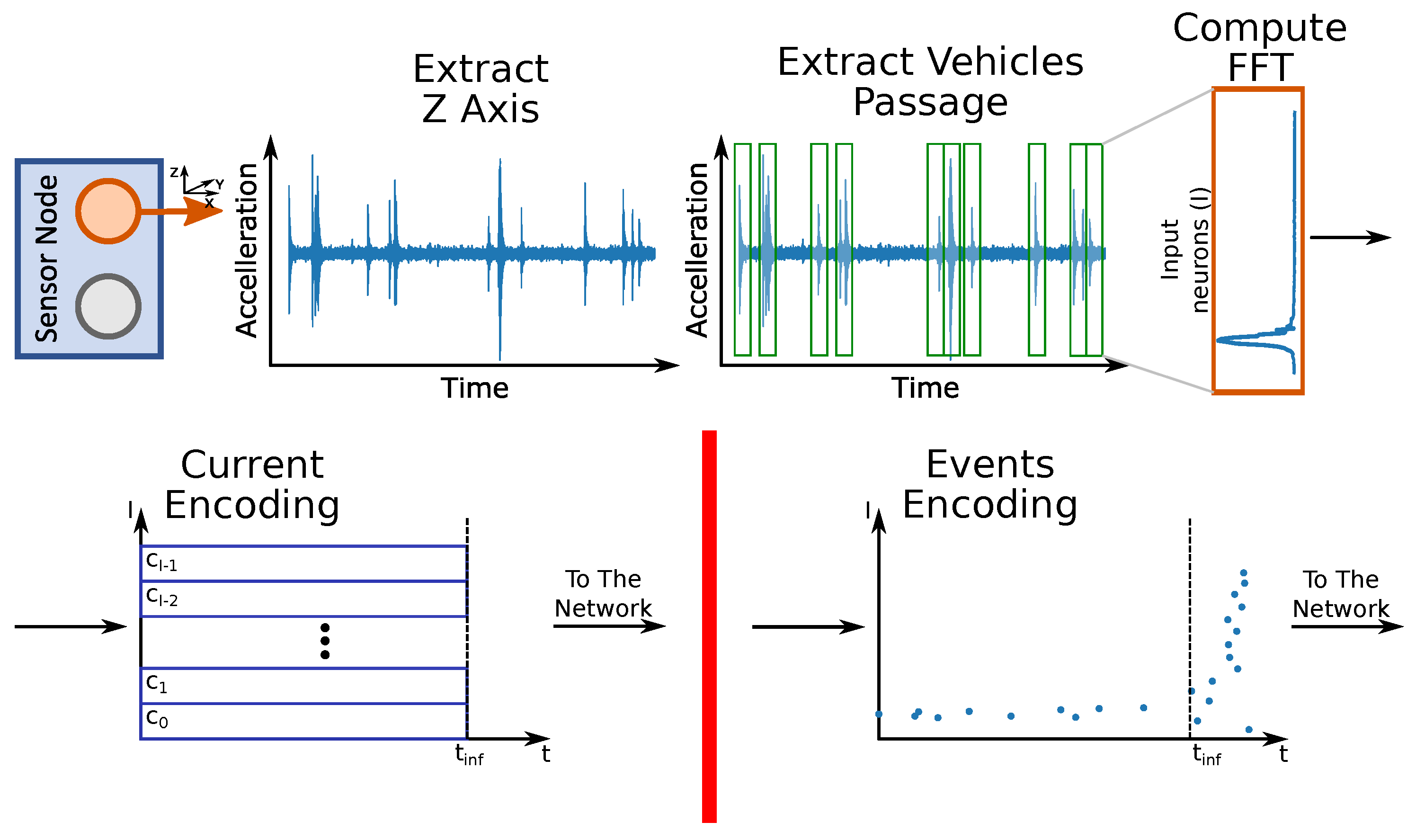
2.4. Input Encoding Methods

The LSNN we used in this work can work with two types of input encodings: Current (current-driven) or events (events-driven). In the Current-Driven LSNN, the input signal is constant for all the inference time, while in the Events-Driven LSNN, the signal is first encoded as spikes and then provided as input. This section describes some of the state-of-the-art encoding methods and details the algorithm we implemented to encode acceleration signals coming from the MEMS sensor. Considering Figure 2, which shows the frequency shift that we want to detect, we give as input to the network the FFT of the acceleration signal due to the vehicle crossing the viaduct.

Literature is rich in algorithms to encode a waveform into a stream of spikes. Some of those approaches try to minimise signal reconstruction error, while others focus on emulating biological-plausible behaviours.

The authors of [29] propose a family of methods that minimise signal reconstruction error. All proposed methodologies are characterised by the presence of two complementary neurons (normally referred to as positive and negative), which expose a contrasting behaviour, that is, when one of the two fires, the other does not.

The simplest temporal encoding algorithm is called Threshold Based Representation (TBR). In this algorithm, whenever the difference between two consecutive signal samples is higher than a predetermined fixed threshold, then the positive neuron emits a spike. Unfortunately, while being computationally cheap to implement, TBR is known for leading to high reconstruction error [29], even for signals with simple dynamics.

The Step Forward (SF) method uses a baseline value (initialised as the value of the first signal sample) and a fixed threshold. Suppose the absolute value of the difference between two consecutive samples is higher than the sum of baseline and threshold. In that case, the positive neuron spikes and the baseline is updated, adding the baseline. A variation of this encoding strategy is called Moving Window (MW), where the baseline is updated looking at a moving window of signal samples. The other encoding methods proposed in [29] have not been considered in this work because of their inherent higher computational complexity that is not suitable for the chosen architectural target.

In [30], the authors describe some biological methods of encoding without considering the reconstruction error. In all these methods, the information is encoded in the reciprocal spikes of several neurons, meaning that proper encoding of the signal depends on the number of neurons adopted. At the time of the first spike, the information is stored in the delay between the start of the stimulus and the neuron’s firing. In this method, the first neuron inhibits all the others; therefore, the information is in just one spike. In latency code, the information lies in the time between spikes of different neurons. In Rank-Order Coding (ROC), the information is encoded in the order of the spikes. In this method, every neuron can fire at most once for every sample (representing a single FFT in our case).

3. Brain Inspired Processing

This section describes the two main components of the brain-inspired processing pipeline, namely input encoding and LSNN architecture. Next section will describe the optimization performed to improve LSNN implementation for edge devices.

3.1. LSNN Input Coding

In the previous section, we discussed possible encoding methods proposed in the literature for LSNNs. In this section, we describe the method we applied to SHM data in our brain-inspired processing pipeline. An example of the input signal is shown in Figure 2.

In Figure 4 the entire data flow is shown. After collecting the data from the sensor, we extract only the z-axis values since they are more sensitive to the vehicles passages. These data are collected with a sampling frequency of 100 Hz and successively downsampled to 12.5 Hz. Subsequently, we get only the windows where vehicles passages have been detected. This was done by thresholding the signal.

The FFT of these windows is computed. The number of input neurons has been selected as two possible values: 50 or 150. This choice was made because a larger number of inputs would have caused a matrix of input weights ($W^I$) too large to train for such a small network, while a smaller number of inputs risks not extracting enough features from the signal [31]. So each vehicle’s window can be composed of 100 or 300 coefficients that, in time, is equal to 8 or 24 s.

FFT coefficients are then given as input to the encoding stage. In the case of Current-Driven encoding, they are provided to the LSNN network one to each neuron for a constant time corresponding to $t_{inf}$. On the other side, in the case of Event-Driven encoding, the ROC algorithm is applied.

Each coefficient is thus encoded as a spike time interval. The larger the coefficient, the smaller the “time-to-spike”. As a result, the spike time interval is inversely proportional to the value of the coefficients. As such, higher coefficients, which are more relevant for the damage detection because they have more energy, will fire first. Lower coefficients will fire later. Since $t_{inf}$ is the inference time for each sample, all neurons that have not fired for $t<t_{inf}$ will no longer be able to fire. This implies that the coefficients with low energy (no information) will not impact the network input. The applied ROC encoding algorithm (Algorithm 1) is shown below:

Algorithm 1: Compute Time-to-Event

The signal S is the sequence of FFT coefficients corresponding to the observed acceleration window made of I coefficients. The inference time $t_{inf}$ is also an input of the algorithm as it is a network parameter.

3.2. LSNN Architecture

The proposed LSNN network is shown in Figure 5, and it is composed of 20 ALIF and two output neurons which discriminate between the two classes of the bridge. We isolated the most important configuration parameters of the training algorithms (hyper-parameters) and studied their impact in terms of LSNN computational complexity and internal activity with an exhaustive search.

The hyperparameters that we explored can be divided into two classes, the network parameters and the training parameters (summarised in

Table 1. LSNN parameters explored.

Parameter	Description	Explored Values
I	Input neurons	50, 150
${\tau }_m$	Recurrent layer membrane potential decay	20, 30
${\tau }_o$	Output layer membrane potential decay	3, 10, 30
$v_{thc}$	Spike threshold coefficient	0.01, 0.03
${\beta }_c$	Adaptive threshold coefficient	1.7, 1.8
${\tau }_{ac}$	Adaptive threshold decay	0.5, 1.0
$t_{inf}$	Inference ticks	5, 10, 20
$re{g}_c$	Loss regularization coefficent	1, 100, 300
$re{g}_r$	Firing rate regularization coefficent	0.01, 0.001

). The first class comprises all the constants that strictly concern the network, while the second class is composed of all the values used to reach better performances but that don’t feature the network. The network parameters that we explored are:

• The input number (I) [50, 150] is the number of input neurons in the first layer. A high number create a huge $W^I$ matrix that cannot be trained by a small network, while a low number risks not extracting all the features of the input signal [31].
• ${\tau }_m$ [20, 30] represents the decay of the membrane potential in the recurrent layer. With high values, the neuron will need more time to return to the resting potential, representing the membrane potential of the neuron if any inputs have not perturbed it.
• ${\tau }_o$ [3, 10, 30] is the decay of the membrane potential of the output neurons.
• $v_{thc}$ [0.01, 0.03]. The spike threshold ($v_{th}$) of the neurons is computing as: $v_{th}=v_{thc}/(1-e^{-\delta t/{\tau }_m})$. A high value of the $v_{thc}$ is translated into a higher value of the threshold.
• ${\beta }_c$ [1.7, 1.8] is used to compute the increase of the adaptive threshold ($\xi$) in the ALIF neurons. Higher values of this parameter are equivalent to a greater increase in the spike threshold.
• ${\tau }_{ac}$ [0.5, 1] is used to compute the decay of the adaptive threshold (${\tau }_a$). ${\tau }_a$ should have a value comparable to the time length of the problem [19].

The training parameters that we explored are the inference time ($t_{inf}$) expressed in ticks [5, 10, 20]. A tick in an SNN represents a cycle to complete the dynamics integration of all network neurons. The actual time depends on the implementation. The inference time is then the number of ticks that the network uses to process the input sample. For the regularisation coefficient we use ($re{g}_c$) [1, 100, 300] and for the regularisation rate we use ($re{g}_r$) [0.01, 0.001]. The two regularisation values are used to computing the loss of the network:

$$L_{fr}={\displaystyle \frac{1}{2}}\sum _j{\left({\displaystyle \frac{1}{nT}}\sum _{t=1}^{nT}{z}_j^t-re{g}_r\right)}^2$$

(5)

$$L=L_p+L_{fr}\ast re{g}_c$$

(6)

Loss is composed of two parts (Equation (6)), the loss of the classification ($L_p$) that is computing with the cross-entropy and the weighted firing-rate loss ($L_{fr}$). The $L_{fr}$ is computed as the difference between the firing rate activity of the network and the $re{g}_r$ that is the desired firing rate [19].

4. eLSNN: The Optimized Embedded LSNN

The implementation of LSNNs was performed taking into account resource constraints and exploiting SNN properties. In particular, sparsity in neuron response (e.g., firing) was exploited in order to skip processing cycles. The firing activity of neurons can be tuned as described in [19] using a loss value dedicated to limit the neuron activity.

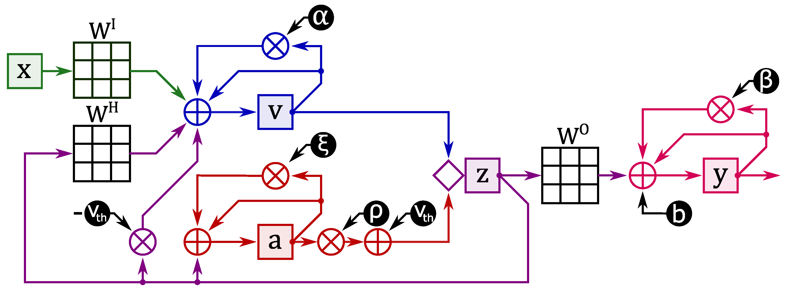
Our LSNN implementation is depicted in Figure 6 and consists of four main steps: (i) Membrane voltage update ($v$), (ii) Membrane voltage threshold update ($a$), (iii) Evaluation of the spike emission ($z$), (iv) Evaluation of the output ($y$). The diagram shows: $x$ data dependencies in green, $v$ data dependencies in blue, $a$ data dependencies in red, $z$ data dependencies in purple and $y$ data dependencies in magenta. In the next sections we will describe in detail the network implementation and the performed optimisations.

4.1. Membrane Voltage Update

The computation involved in the membrane voltage update ($v$), as shown in Figure 6 in the first blue ⊕ operator, is done through the following steps:

• Membrane voltage decay: $v^{\left(\alpha \right)}:=\alpha v$
• Contribution of inputs on membrane voltage: $v^{\left(I\right)}:=W^{I}x$
• Contribution of internal neuronal activity on membrane voltage: $v^{\left(H\right)}:=W^{H}z$
• Reduction of membrane voltage in case of previous spike emission: $v^{\left(th\right)}:=-v_{th}z$
• Update of membrane voltage: $v\leftarrow v+v^{\left(\alpha \right)}+v^{\left(I\right)}+v^{\left(H\right)}+v^{\left(th\right)}$

In

Table 2. Operations analysis for a single neuron. These operations must be executed for each neuron (N) and for each inference tick ($t_{inf}$).

Item		Naive				Optimised
		Sum	Mul	Store		Sum	Mul	Store
$v^{\left(\alpha \right)}$		-	1	-		-	1	-
$v^{\left(I\right)}$		I - 1	I	-		$\tilde{x}$ - 1	-	-
$v^{\left(H\right)}$		N - 1	N	-		$\tilde{z}$ - 1	-	-
$v^{\left(th\right)}$		-	1	-		1	-	-
$v$		4	-	1		4	-	1
Total		I + N + 2	I + N + 2	1		$\tilde{x}$ + $\tilde{z}$ + 3	1	1

we report the operations (sum and multiply) of both the non optimized (Naive) and optimised version for each component of $v$. Overall, the operations to be performed are: $(I+N+2)N{t}_{inf}$ sum and $(I+N+2)N{t}_{inf}$ multiplication.

Because of the event-driven design of the network, it is possible to implement the computation of the $v^{\left(I\right)}$ and $v^{\left(H\right)}$ components more efficiently. Considering the row-column multiplication between the matrix W (with $N\times M$ elements) and the column vector $x$ (with $M\times 1$ elements), the operation result will be added to the vector $v$. When the elements of $x$ can only assume binary values ($x_i\in \left\{0,1\right\}$) the $Wx$ operation can be implemented using only sums. The following pseudo-code formally describes the operation:

Let $\breve{x}$ be a list containing only the index of the non-zero elements of $x$. By iterating over the elements of $\breve{x}$ we select the columns of W to be considered in the sum cycle (inner cycle). The sum cycle iterates over the rows of the selected column, and for each element accumulates its content in the result vector. The required operations will therefore be dependent on the number of non-zero elements in the vector $x$. The number of non-zero elements in the vector $x$ will change with each inference tick. We then identify using the symbol $\tilde{x}$ the average number of non-zero elements of $x$ for each inference tick.

We then reduce the sums required for the membrane voltage update from $(I+N+2)N{t}_{inf}$ to $(\tilde{x}+\tilde{z}+3)N{t}_{inf}$ and the multiplications from $(I+N+2)N{t}_{inf}$ to $N{t}_{inf}$. The value of $\tilde{x}$ depends on the chosen event encoding. The value of $\tilde{z}$ depends on the behaviour of the network. When training the network, it is possible to minimise $\tilde{z}$ by introducing its value into the loss calculation.

4.2. Threshold Update

Updating the threshold for the membrane voltage ($a$), as shown in Figure 6 in the first red ⊕ operator, is broken down into the following operations:

• Evaluation of threshold decay: $a^{\left(\xi \right)}:=\xi a$
• Threshold adjustment in case of previous spike: $a^{\left(z\right)}:=z$
• Threshold update: $a\leftarrow a+a^{\left(\xi \right)}+a^{\left(z\right)}$
• Weighted threshold computation: $a^{\left(\rho \right)}:=\rho a$
• Reference threshold augmentation $v_{th}^{\left(a\right)}:=v_{th}+a^{\left(\rho \right)}$

In total, $3N{t}_{inf}$ sums and $2N{t}_{inf}$ multiplications are required to implement the adaptive threshold functionality.

4.3. Spike Emission Check

At each inference tick, the spike firing condition must be checked. For each neuron, the membrane voltage is compared with the spike threshold. In this particular implementation, the threshold voltage is adapted to the activity of the neuron and increases as its activity increases. A spiking neuron is also inhibited for a period $t_{ref}$ called refractory time. Even if the neuron has a membrane voltage above the threshold during this period, it will not fire. To check this condition, each neuron stores the information about the tick of the last spike $t_i^{\left(z\right)}$.

When checking the emission of a spike, as shown in Figure 6 in the first purple ◊ operator, two conditions must therefore be checked for each neuron:

• The membrane voltage must be above the adaptive threshold: $v_i\ge v_{th}^{\left(a\right)}$
• The neuron must not be inhibited by an earlier spike: $t\ge t_i^{\left(z\right)}+t_{ref}$

If the above conditions are satisfied, the vector $z$ will take the value 1 at position i, otherwise the value 0.

In our implementation, instead of directly handling the vector $z$, we use the list of events $\breve{z}$. Using the list of events, we can replace matrix multiplications $W^{H}z$ and $W^{O}z$ with sums. At the beginning of the spike emission check phase, the list $\breve{z}$ of previous events are cleared. In the presence of a spike emission, the identifier of the spiking neuron will be added into the $\breve{z}$ list.

4.4. Output Update

Output neurons receive spikes generated by network neurons in the recurrent layer at the same tick as they are emitted. As shown in Figure 6 in the first magenta ⊕ operator, the output neurons have a similar update cycle to the recurrent neurons:

• Output decay: $y^{\left(\beta \right)}:=\beta y$
• Contribution of internal neuronal activity on output: $y^{\left(H\right)}:=W^{O}z$
• Bias contribution: $y^{\left(b\right)}:=b$
• Update of output: $y\leftarrow y+y^{\left(\beta \right)}+y^{\left(H\right)}+y^{\left(b\right)}$

Again, the calculation of $y^{\left(H\right)}$ requires a multiplication between the matrix $W^O$ and the vector $z$. The procedure described in Section 4.1 helps to lower the number of operations. Using the list $\breve{z}$ it is possible to solve the operation $W^{O}z$ using sums only. The number of operations is then lowered from $(N-1)O{t}_{inf}$ sums and $NO{t}_{inf}$ multiplications to $\tilde{z}O{t}_{inf}$ sums.

4.5. Current-Driven Input

In this work, we consider also an alternative to input events, using continuous (e.g., real) values in the vector $x$ [19]. While in this case it is not possible to perform the optimisations described in Algorithm 2 for solving $v^{\left(I\right)}:=W^{I}x$, we provide an optimised version of the LSNN using this type of input to evaluate the trade-offs lead by the two encoding methods and reported in Section 5. We note that in this case the contribution of internal neuronal activity $v^{\left(H\right)}$ (hidden/recursive layer) is still spike-based, however in the input-layer it is not possible to remove multiply operations as it is possible using input spike events.

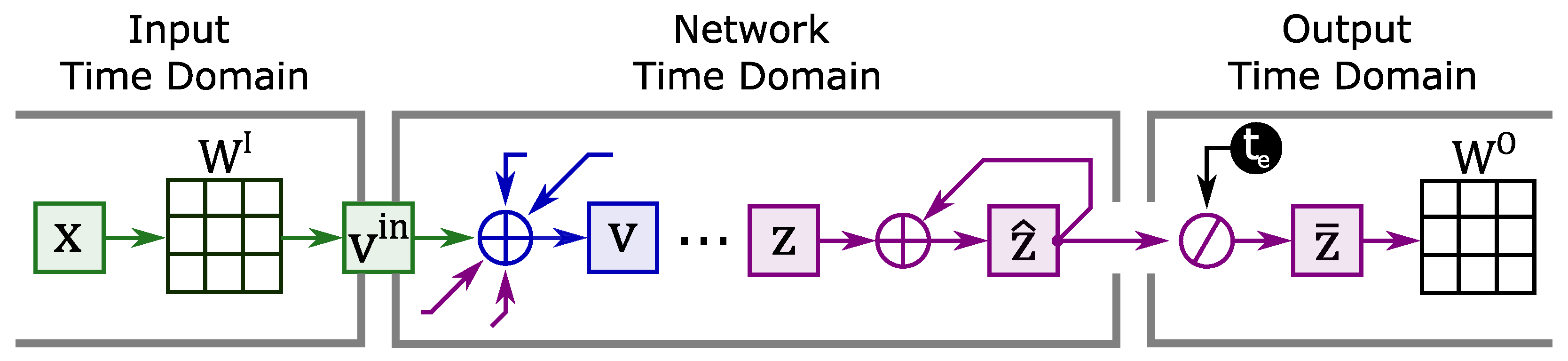
In the literature, networks using continuous input typically observe a sample for a period called the exposure time $t_{exp}$. Within the network exposure time, the same values of $x$ are always presented. This leads to the formation of three time domains (although it is common for the time domains of input and output to coincide) represented in Figure 7:

• Temporal domain of the input, where the input varies over time.
• Temporal domain of the network, for each tick in the input-time-domain the network performs $t_{exp}$ iterations always observing the same value of $x$
• Temporal domain of output, where output varies over time.

Algorithm 2: Optimized implementation of $v\leftarrow Wx$ when x is a boolean vector.

In order to efficiently handle this LSNN variant, the time domains are decoupled by vectors $v^{in}$ and $\widehat{z}$. The first vector decouples the input from the network; it is computed by a row-column multiplication between the matrix $W^I$ and the vector $x$ each time the input changes. Then, the vector $v^{in}$ will be used to increment $v$ at each tick of the network. The number of operations to compute $v^{\left(I\right)}$ then becomes $(1/t_{exp}(I-1)N+N)t_{inf}$ sums and $t_{inf}/t_{exp}IN$ multiplications.

The second vector decouples the network from the output. The output will no longer process the spikes coming from the network but will use the average activity of the network within the exposure time as information. At each tick, the network must accumulate the emitted spikes inside the vector $\widehat{z}$. In the time domain of the output the content of the vector will be averaged ($\overline{z}$) and used for the calculation of $y^{\left(H\right)}:=W^O\overline{z}$.

The number of operations for calculating $y^{\left(H\right)}$ then becomes $(1/t_{exp}(N-1)O+\tilde{z})t_{inf}$ sums and $t_{inf}/t_{exp}NO$ multiplications.

In the following, we will refer to this LSNN version as current-driven eLSNN, since the continuous and constant input over the exposure time can be interpreted as a constant current stimulus. The version working with input spikes (e.g., binary values) will be referred to as event-driven eLSNN instead.

5. Experimental Result

This section first describes the experimental setup used to test the LSNN implementation presented in the previous sections. Then, it reports the results of the design trade-off characterisation for the proposed eLSNN. In particular:

• Section 5.1 describes the hardware-in-the-loop system we implemented to profile the runtime and energy performance of the SHM application.
• In Section 5.2, we study the accuracy of the trained eLSNNs (current-driven and event-driven). We evaluated the MCC on the test dataset for the first order hyper-parameters, which impact the energy and computational efficiency of the eLSNN implementation. The first-order hyper-parameters are the input number (I) and inference ticks ($t\_inf$) of the networks.
• In Section 5.3, we study the impact of the eLSNN performance ($\#executioncycles$) considering the most accurate networks for each eLSNN version (current-driven and event-driven). We also considered different combinations of the first-order parameters as a function of the activity factors of the eLSNNs (number of non-zero elements (spikes), both in the input (x) and hidden/recurrent layer z).
• In Section 5.4, we perform a complete characterisation of the SHM sensing node firmware for a network implementation having median activity-factors. This corresponds to a typical behaviour of the sensor node for a real SHM application in terms of execution time and energy-consumption.

5.1. Testbed

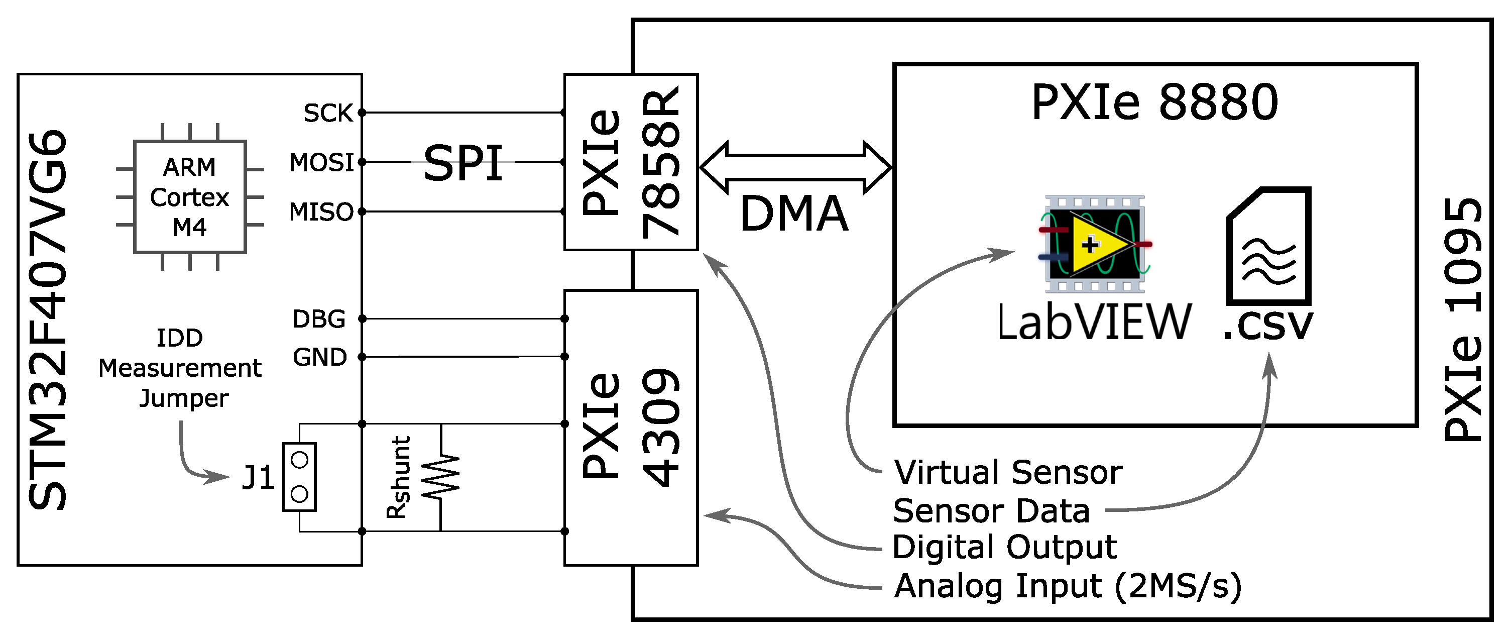
We prepared a hardware-in-the-loop setup to characterise the performance and energy of the data acquisition and processing board. As shown in Figure 8, the testbed we implemented is composed of three actors: (i) A development board hosting the STM32 MCU (System-on-Chip) on the left; (ii) A data acquisition system to monitor the consumption of the STM32 development board (Analog Input) on the right and (iii) A FPGA emulation module able to feed the processing unit in the system-on-chip with data coming from the real-world SHM application described in Section 2 in real-time (Virtual Sensor). (based on PXIe systems from NI [32]).

Both the Analog Input and the Virtual Sensor are part of a PXIe systems from NI [32]). This is a modular, LabVIEW controlled environment able to perform fast measurements requiring high-performance digital and analog I/O. The following three subsections provide further details about the PXI modules used in the experimental setup and their role in the pipeline characterisation.

5.1.1. System-on-Chip

We implemented and deployed the entire SHM pipeline on an STM32F407VG6 MCU. It is a system-on-chip manufactured by STMicroelectronics, which features an ARM Cortex-M4 with a floating-point unit. The core comes with 192 KB RAM and 1 MB FLASH memory and supports a maximum clock frequency of 168 MHz. The STM32F407VG6 supports multiple low-power modes and various clock frequency configurations, which allow a fine-grained tuning of the system performance depending on the application needs. For the sake of this work, we apply the following policies:

• When the system is in RUN mode, the system-on-chip is always clocked at the maximum allowed clock frequency, equal to 168 MHz.
• When the system fetches data from the MEMS sensor over SPI, the transfer is performed via DMA with the core in SLEEP mode. Before entering SLEEP mode, the MCU core is clocked down to 16 MHz to minimize SLEEP current consumption.
• When the system-on-chip is not working, it is put in STANDBY mode, switching off the voltage regulator to achieve the lowest consumption possible. Notice that we can apply such an aggressive power-saving policy since we assume our SHM application does not need to retain any state before one LSNN inference and the next inference.

Considering the software stack employed to implement the SHM application, we interfaced the on-board peripherals using the Hardware Abstraction Layer provided by STMicroelectronics. Instead, the mathematical processing (e.g., FFT computation, FFT-to-spike conversion) is implemented using the CMSIS-DSP library primitives. It is a set of routines developed by ARM to deliver DSP-like functions optimized to run on Cortex cores.

5.1.2. Analog Input

The power and performance monitoring activity of the pipeline has two requirements: (i) Measure the current sunk by the system-on-chip at any time of the data acquisition and processing and (ii) precisely split the current waveform into each pipeline stage, to detect the analysis stages that are the more power hungry or require most MCU cycles to be accomplished. Both requirements are met by using a PXIe-4309 ADC device reading 2 M Samples per second and featuring 32 channels 18 bit wide. We used two of the available input channels to perform the following synchronous activities:

• Sample the current sunk by the MCU using a 1 Ohm shunt resistor. Such measurement exploits a jumper available on the development board to monitor current consumption on the VDD of the system-on-chip.
• Read the logic level of a debug GPIO (DBG pin, Figure 8) that is toggled by the application software each time a processing stage is started or completed, to associate each phase (e.g., SPI transfer, FFT computation, SNN inference) to its current consumption waveform (with negligible overhead on the application performance).

5.1.3. Virtual Sensor

The Virtual Sensor is an FPGA-based emulation system that allows feeding the SPI interface of the MCU with data taken from a trace. The trace was obtained from a real sensor deployment on the field. For characterisation and profiling purposes, the virtual sensor was connected to the MCU replacing the MEMS present in the sensor node board. The Virtual Sensor is completely implemented within the PXI system and is made of two modules sharing data through a DMA-controlled hardware FIFO:

• PXIe-8880: The PXI system controller, which is a general-purpose CPU-based host running Windows 7 and LabVIEW. It loads the accelerations measured on the bridge from a CSV file and pushes them into a FIFO at the boundary of the FPGA system.
• PXIe-7858R: The PXI FPGA module, which loads the measurements the DMA move from the controller to its FIFO. It acts as a digital MEMS that samples structural accelerations at a constant rate and stores them in an on-board buffer which can be accessed in-order through an SPI interface.

5.2. Accuracy vs. First-Order Hyper-Parameters

As introduced in Section 2, to study the impact of the eLSNNs hyper-parameters and flavours on the accuracy, we conducted an exhaustive search. We evaluated the accuracy as the Matthews Correlation Coefficient (MCC) on the test set, which includes all the samples related to vehicle passages on the bride section during a randomly chosen day before and after the scheduled maintenance intervention.

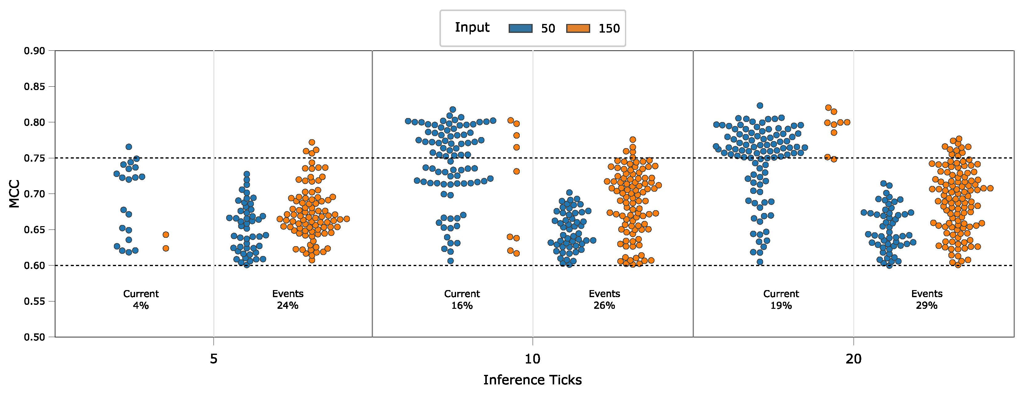
In Figure 9, we report on the y-axis the network accuracy measured as MCC. We limited the plot to those hyper-parameters configurations leading to eLSNNs with an MCC $\ge 0.6$. This corresponds to an accuracy of 0.77. Moreover, in the same figure, we draw the line at the MCC $=0.75$. We consider all the eLSNNs configurations achieving an MCC higher than 0.75 as acceptable or “good” configurations. This threshold corresponds to accuracy above 0.88.

On the x-axis, we report three sets of plots. Each set corresponds to different inference ticks ($t_{inf}=5,10,20$). Inside each set, the left plot refers to the current-driven eLSNN, and the right plot refers to the event-driven eLSNN. Inside each of these plots, we report the eLSNN configurations achieving a MCC $>0.6$. The percentage of these configurations on the total evaluated (1728 for each eLSNN flavour) is reported in the text on each plot’s bottom. The MCC accuracy of each configuration is reported with red bins for an input number of 50 and with blue bins for an input number of 150 bins. In the SHM application, the input number (I) corresponds to the magnitude of the spectral components of the FFT. It thus is equal to the double of the accelerations samples, which needs to be read by the sensor to compute an eLSNN inference.

The combination of these parameters ($t_{inf} \& I$) constitutes the first-order hyper-parameter that, as we will see in the next section, impact the inference execution time of the eLSNNs and then their energy consumption. From the figure, we can notice that for the current-driven eLSNNs, the largest number of acceptable configurations is achieved for an input number (I) of 50. Which also corresponds to the lower complexity of the eLSNN computations (see Section 4). Differently, for the event-driven eLSNNs, acceptable configurations can be achieved only with an input number (I) of 150. As we will see in Section 5.4, this has a severe drawback on the pre-processing cost for this eLSNN flavour. It is also worth to note that for the current-driven eLSNNs the accuracy improves with larger inference ticks, having any acceptable configurations with $I=50$ and $t_{inf}=5$ but several with $I=50$ and $t_{inf}=10,20$. However, this is not the case for the event-driven eLSNNs for which their MCC does not improve significantly with progressive $t_{inf}$ increases. It is now interesting to evaluate these parameters’ impact in terms of eLSNN inference execution cycles.

5.3. Execution Time vs. Activity-Factors

As described in Section 4, the optimised eLSNN algorithm we propose in this paper leverages the sparse nature of the spikes for saving computations. If a neuron does not receive a spike, it does not trigger accumulation in the membrane potential. This means that the computational burden of the eLSNN algorithm depends on the average number of non-zero elements for each inference tick in the recursive/hidden layers. This is true for both current-driven and event-driven eLSNNs. For the event-driven eLSNN only, also the input layer must be considered in this computation. To understand the relevance of these effects on the total eLSNN inference time, we have to analyse different input samples. Each sample corresponds to the FFT coefficients of the accelerations read by the MCU during a passage of a vehicle. More specifically, the number of spikes corresponding to non-zero elements in the recurrent layer during an eLSNN inference (denoted with z) depends on the specific input sample and network hyper-parameters. Differently from the recurrent/hidden layer activity (z), the input activity factors vary between the eLSNN flavour. For the current-driven eLSNNs, the input activity depends only on the input number (I). In contrast, for the event-driven eLSNNs, the input layer activity depends on the input spikes and non-zero elements in the coded inputs for all the ticks (x). x depends on the input sample and input number (I) as it is a property of the spiking input encoding.

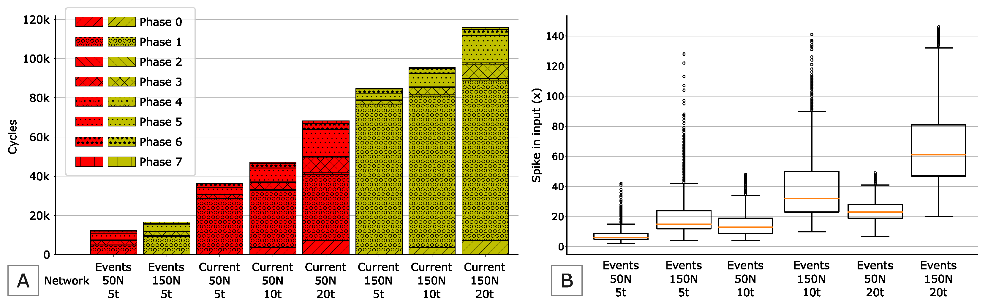
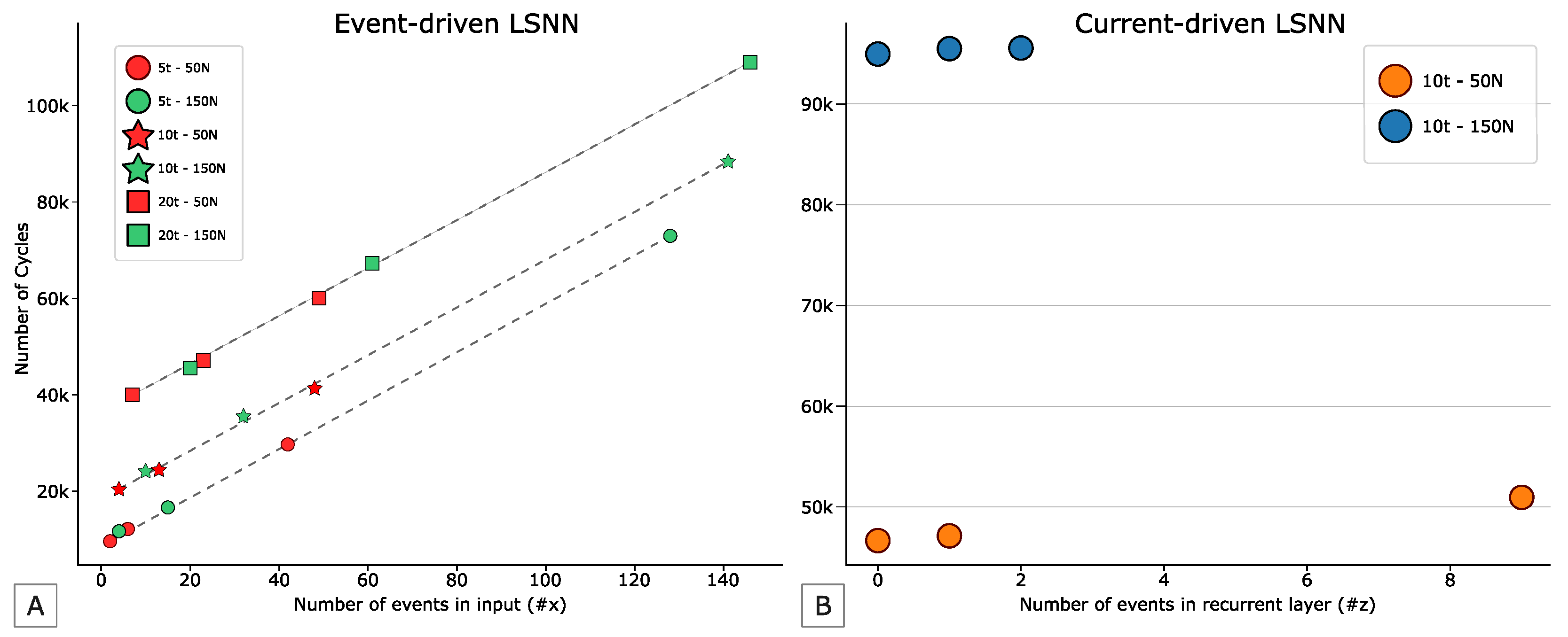
Figure 10B reports on the y-axis the total number of cycles needed by the eLSNN to complete one inference computation on a given input sample. This number of cycles accounts only for the eLSNN computation after the pre-processing step. On the x-axis, we report the value of z, which corresponds to the number of spikes/events/non-zero elements in the recurrent/hidden layer integrated into all the inference ticks ($t_{inf}$).

The different colours refer to the two different networks selected among the many with acceptable performance. For each type of network, we selected the ones with a number of inputs (I) leading to the largest (z) variation among the input samples in the test set.

Then, we plot three values of z chosen for each network corresponding to the minimum, the maximum, and the median sample. From the plot, we can notice that the impact of the z is negligible with respect to the total execution time of the eLSNN inference. Differently, the inference time for current-driven eLSNN halves when reducing the input number I from 150 to 50. As the impact of z is negligible, we can ignore its effect in the following plots.

Figure 11B reports on the y-axis the distribution of the non-zero elements in the input layer for each input sample in the test set for event-driven eLSNNs. The distribution depends on the input element and the encoding, which depends on the first-order hyper-parameters, namely the inference ticks ($t_{inf}$) and the number of inputs (I). In the y-axis, we report the different configurations of the first-order hyper-parameters. From the plot, we can see that the number of events/spikes/non-zero elements in the input layer (x) is more significant and has higher variability than the same quantity in the recurrent/hidden layer (Figure 10B). Moreover, the number of input events/spikes/not-zero elements increases both in average and standard deviation with the increase of the input number and inference ticks.

Figure 10A reports for each of the different configurations of the first-order hyper-parameters and for the input sample corresponding to the minimum, maximum and median values of x the execution time of the event-driven eLSNN. We can see that both the first-order hyper-parameters vary the execution time. The execution time increases linearly with the inference ticks and with x. It is interesting to notice that for the event-driven eLSNNs, the input number (I) does not increase the execution time directly as with the current-driven eLSNNs but indirectly. Indeed, a larger input number (I) increases the execution time proportionally to the increase of x. Which eLSNN flavour and configuration should thus be preferred?

5.4. Event-Driven vs. Current-Driven

This section concludes the eLSNN study by comparing the performance of the most performing and energy-efficient current-driven, and event-driven eLSNN averaged on the test set. This is obtained by evaluating the candidate eLSNNs in the median sample with respect to both x and z.

Figure 11A reports on the same plot the breakdown of the total number of cycles taken by the median inference time of both the current-driven and event-driven eLSNNs. For the current-driven networks, all the first-order hyper-parameters combinations are reported, while for the event-driven eLSNNs, we report only the configurations with inference ticks equal to 5, which corresponds to the most energy-efficient networks. By comparing the different networks, we can notice that the two most performing eLSNNs which achieves MCC $\ge 0.75$ are the configuration $I=150,t_{inf}=5$ for the event-driven eLSNN and $I=50,t_{inf}=5$ for the current-driven eLSNN. The event-driven eLSNN requires less than half of the cycles of the current-driven eLSNN. We can conclude that event-driven eLSNN is significantly more efficient (>$50\%$) than the current-driven eLSNN. It must be noted that this conclusion does not account for the pre-processing of the input sample (affecting the input number) which is more significant for the selected event-driven eLSNN. It is interesting to notice that the event-driven eLSNN configured with $I=50,t_{inf}=5$ is the most efficient one, but its MCC is lower (0.72) than the accuracy threshold of MCC ≥ 0.75. Moreover, in the Figure 11A we report with different patterns the number of cycles needed to perform the computational steps described in Section 4.

• Phase 0: Compute of $v^{\left(\alpha \right)}$
• Phase 1: Compute of $v^{\left(I\right)}$
• Phase 2: Compute of $v^{\left(H\right)}$
• Phase 3: Compute of $a^{\left(\xi \right)}$
• Phase 4: Compute of $a^{\left(th\right)}$ and $a^{\left(z\right)}$
• Phase 5: Compute of $z$ and insert items in $\breve{z}$
• Phase 6: Compute of $y$
• Phase 7: Insert items in $\breve{x}$ for next iteration.

For the current-driven eLSNN the Phase 1 dominates the computational time since it must compute the $v^{in}$ vector by means of a complete matrix-vector multiplication. Phase 0 and Phase 3 involves N multiplications, and at increasing $t_{inf}$ their execution times become increasingly evident.

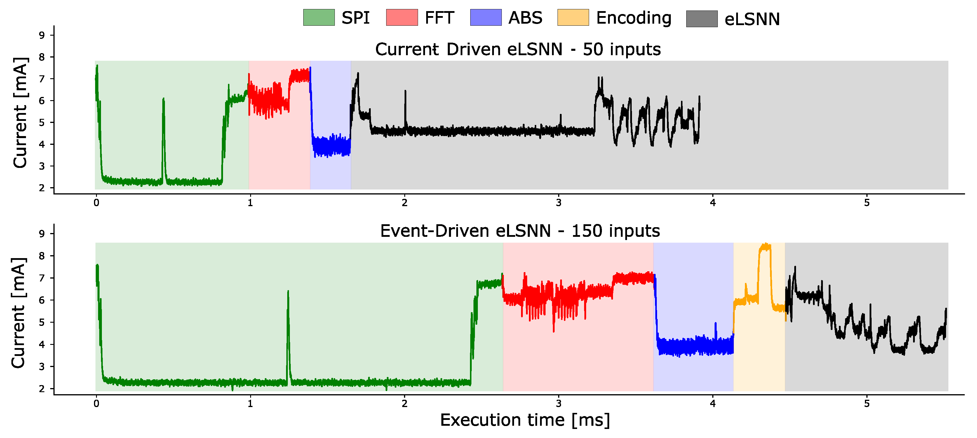
Figure 12 shows the MCU’s current consumption when executing the entire processing steps needed to read the sensor values through the SPI interface, pre-process the sample (FFT + ABS), and compute the eLSNN kernel. We report the current-driven eLSNN in its most efficient configuration on the left plot, and on the right plot, we report the event-driven eLSNN in its most efficient configuration. Even if the event-driven eLSNN kernel costs halves of the cycles than the current-driven eLSNN, it requires three times more sensor’s readings to compute an inference for an input sample. This increases the cycles needed to read the sensor’s data in SPI and compute the FFT and abs. Moreover, the event-driven eLSNN requires an additional pre-processing step consisting of the coding of the spectral components in spikes/events described in Section 3.

As described in Section 4.5 the version of the network with current input needs a matrix-vector multiplication for each input tick $t_{inp}=t_{inf}/t_{exp}$. In this use case, we have only one input tick and only one matmul is executed, but it is enough to increase the number of cycles considerably. In Figure 12 top it is possible to appreciate this phase because it is visible for a long period (around milliseconds 2 and 3) not present in Figure 12 bottom.

Table 3. Power report of the SHM application featuring the best eLSNNs tested. The SPI master transfers data with a serial clock of 8 MHz. The SPI stage includes: (i) The SPI data transfer, (ii) the time required by the system-on-chip to reconfigure the clock to 168 MHz when it wakes-up from SLEEP mode and (iii) the conversion of sensor data from raw integers to floating-point.

Stage	Current-Driven
	Time [$\mathsf{\mu }$s]	Cycles [#]	Current [mA]	Power [mW]	Energy [$\mathsf{\mu }$J]
SPI	542	-	5.01	16.53	8.96
FFT	41	6971	38.76	127.91	5.24
ABS	26	4284	36.58	120.71	3.14
Encoding	-	-	-	-	-
eLSNN	215	36,036	40.26	132.86	28.56
Total	824	47,291	-	-	45.90
Mean	-	-	16.88	55.70	-

and

Table 4. Power report of the SHM application featuring the best eLSNNs tested. The SPI master transfers data with a serial clock of 8 MHz. The SPI stage includes: (i) The SPI data transfer, (ii) the time required by the system-on-chip to reconfigure the clock to 168 MHz when it wakes-up from SLEEP mode and (iii) the conversion of sensor data from raw integers to floating-point.

Stage	Current-Driven
	Time [$\mathsf{\mu }$s]	Cycles [#]	Current [mA]	Power [mW]	Energy [$\mathsf{\mu }$J]
SPI	949	-	4.33	14.29	13.56
FFT	101	16,968	38.17	125.96	12.72
ABS	50	8316	35.97	118.70	5.94
Encoding	32	5459	42.65	140.75	4.50
eLSNN	99	16,631	38.20	126.06	12.48
Total	1231	47,374	-	-	49.20
Mean	-	-	12.11	39.97	-

summarises all these effects. We can notice that even if the event-driven eLSNN kernel takes $54\%$ fewer cycles than the current-driven eLSNN network, the total computation time is 1.51× longer for the event-driven eLSNN. This is primarily due to the SPI transfer, which is 2× longer than for the current-driven eLSNN. Even with this extra execution time, the total time for computing the network matches the real-time requirements of the SHM application. Due to the lower power cost of the SPI transfer (w. DMA), however, the energy-consumption for the eLSNN flavours ( event-driven and current-driven inputs) is comparable and in the range of 46–49 $\mathsf{\mu }$J.

In future works, we will explore temporal coding techniques and migrate the coding task directly in the MEMS sensor and in the time domain. These on-sensor coding techniques will remove the FFT cost and the amount of data to be read from the MEMS sensors, achieving further energy reduction in the sensor node.

6. Conclusions

In this paper, we presented an optimised implementation of a recurrent Spiking Neural Network on embedded microcontrollers for damage detection in Structural Health Monitoring applications. We studied the feasibility of spiking based processing and the trade-offs involved in using an event-based input. Thanks to this implementation, called eLSNN, we were able to design, implement and characterise an SNN-based monitoring system, where the computation is performed near to the sensor node. We described the optimisations we performed with respect to a naive LSNN algorithm present in the state-of-art to reduce computation cycles and improve energy efficiency. We also studied two alternative encodings of the input, showing how they impact performance and energy. We highlight the trade-offs between eLSNN execution and data transfer costs that have to be explored to select the best energy/performance configurations. Results of accuracy obtained on a real use case demonstrated that LSNN is a viable solution for damage detection in SHM, having high accuracy ($\mathrm{MCC}\ge 0.75$) and low cycle and energy overheads if compared with the data transfer costs. Moreover, the results highlight that moving the spike-coding directly in the sensor can lead to even more energy-efficient implementation. The eLSNN working with input spikes is more energy-efficient than the one using real (continuous) values. The promising results in this work open the way to the implementation of SNN-based processing on-edge. Moreover, when compared with a state-of-art work leveraging an autoencoder (ANN) on the same dataset [7], the proposed eLSSN approach shows lower complexity (from 32,000 MAC operations to 15,750 sums and 750 multiplications).

Future work will be devoted to evaluating and comparing event-based SNN approaches against other SHM datasets and comparing extensively with ANN algorithms.