Cross-Project Defect Prediction Method Based on Manifold Feature Transformation

Abstract

Traditional research methods in software defect prediction use part of the data in the same project to train the defect prediction model and predict the defect label of the remaining part of the data. However, in the practical realm of software development, the software project that needs to be predicted is generally a brand new software project, and there is not enough labeled data to build a defect prediction model; therefore, traditional methods are no longer applicable. Cross-project defect prediction uses the labeled data of the same type of project similar to the target project to build the defect prediction model, so as to solve the problem of data loss in traditional methods. However, the difference in data distribution between the same type of project and the target project reduces the performance of defect prediction. To solve this problem, this paper proposes a cross-project defect prediction method based on manifold feature transformation. This method transforms the original feature space of the project into a manifold space, then reduces the difference in data distribution of the transformed source project and the transformed target project in the manifold space, and finally uses the transformed source project to train a naive Bayes prediction model with better performance. A comparative experiment was carried out using the Relink dataset and the AEEEM dataset. The experimental results show that compared with the benchmark method and several cross-project defect prediction methods, the proposed method effectively reduces the difference in data distribution between the source project and the target project, and obtains a higher F1 value, which is an indicator commonly used to measure the performance of the two-class model.

1. Introduction

Currently, the complexity of software is increasing, which is mainly reflected in the continuous increase in the number of developers and the scale of the software system. The increase in personnel and scale will inevitably lead to more hidden defects in the software system. However, a comprehensive test of a complex software system requires a considerable amount of resources. Therefore, we hope to know the defect tendency of each module of the software system in advance so as to allocate the test resources of each module in a targeted manner. Software defect prediction technology [1,2,3,4,5] can help us achieve this goal. Through software defect prediction technology, we can predict the defects of each module of the software project. If the predicted module is defective, then we will focus on testing the module so as to achieve the purpose of allocating testing resources for each software module in a targeted manner.

Software defect prediction technology is used to build a software defect prediction model with the help of machine learning methods. The training data are the value of the measurement features extracted from software modules, such as CK metrics [6]. The current research on within-project defect prediction (WPDP) [7,8,9,10] has been established, but WPDP cannot be practical because WPDP requires part of the defect data of the same project or the historical version of the project. However, the software developed in practice is generally a brand new software project, and the brand new software project does not have historical version data. Machine learning methods are data-supported methods; thus, WPDP lacks practicality in the absence of training data.

In view of the lack of training data, researchers have proposed cross-project defect prediction (CPDP) [11,12,13]. CPDP is based on the labeled defect data of other similar software projects (i.e., source project) to train the model and predict the defects of the software projects under development (i.e., target project). However, due to the large differences in the data distribution of the source project and the target project, the defect prediction model constructed using the source project data cannot achieve good predictive performance on the target project. Therefore, how to reduce the difference in data distribution between the source project and the target project has become the focus of CPDP research.

Researchers have proposed a variety of methods and models to reduce the difference in data distribution between projects to improve the performance of CPDP. These efforts include the Burak instance filtering method [14] and Peters instance filtering method [15] based on similarity training data selection, the TNB model based on instance weighting proposed by Ma et al. [16], the large-scale combination model HYDRA based on searching the best instance weights proposed by Xia et al. [17], the source project training data selection method CFPS based on collaborative filtering proposed by Sun et al. [18], the TCA+ method based on feature space transformation proposed by Nam et al. [19], the method based on feature matching and migration proposed by Yu et al. [20], the cross-project defect prediction method based on feature migration and instance migration proposed by Ni [21], etc.

In the above methods, we found that research from the perspective of feature space transformation or feature migration can greatly improve the performance of CPDP. However, the results achieved so far are not very satisfactory. The reason for our analysis is that the feature transformation is to map the source project and the target project from the original feature space to the common feature space, and feature migration is to match the features of the source project to the features of the target project in the original feature space. These methods perform feature transformation and feature migration in the original feature space. Additionally, the original feature space has feature distortions, which results in the data distribution between the transformed source project and target project not being effectively reduced. Therefore, the effect of feature transformation and migration will be restricted. These problems are also very common in the field of image recognition [22]. Related researchers [23,24] proposed a method to measure the distribution of different domains in the manifold space and reduced the drift between domains, which effectively improves the accuracy of image classification.

Inspired by this, we introduce the method of manifold feature transformation and propose a cross-project defect prediction method based on manifold feature transformation (i.e., MFTCPDP). Specifically, first, the original feature space was transformed into manifold space, and then the data distribution difference between the source project and the target project in the manifold space was reduced. Finally, the classifier was constructed by using the source project data and labels in the manifold space to predict the defects of the target project. In order to demonstrate the effectiveness of the MFTCPDP method, we conducted experiments on the Relink datasets and the AEEEM datasets to conduct experimental research on the overall performance of the method. The experimental results show that the prediction performance of the MFTCPDP method is better than the benchmark method and has certain advantages, compared with several CPDP methods.

The rest of the paper is organized as follows: Section 2 briefly introduces the existing methods in the field of cross-project defect prediction. Section 3 introduces the cross-project defect prediction method based on manifold feature transformation proposed in this paper in detail. Section 4 conducts empirical research on the methods proposed in this paper, including evaluation objects, evaluation indicators, experimental settings, and experimental results and analysis. Section 5 summarizes the full text and presents the next steps.

2. Related Work

In recent years, CPDP research has attracted widespread attention from software engineering researchers. Briand et al. [25] conducted a feasibility study on CPDP for the first time and discussed whether CPDP is worth studying. Finally, they found that CPDP research is very valuable and very challenging. Subsequently, Zimmermann et al. [26] conducted a large-scale experimental study on CPDP research and found that most of the experimental results had poor performance, and only a few CPDP experiments achieved satisfactory performance on a variety of indicators. Since then, researchers have proposed various methods to improve the performance of CPDP from different angles.

Some researchers choose suitable training data for the target project based on the similarity measure. He et al. [27] and Herbold et al. [28] calculated the values of the features of each project on a variety of statistical indicators, such as mode, average, variance, etc., constructed a new distribution vector, and then selected the most similar source project for the target project as the training data by calculating the difference of each distribution vector. Turhan et al. [14] proposed a Burak filtering method based on target project instances, which, in turn, selected the most similar k instances from candidate source projects for each instance in the target project to obtain training data. Peters et al. [15] proposed a similar instance filtering method. The difference is that Peters et al. used a clustering algorithm to select training data from source project instances.

Some researchers solve the problem of data distribution differences between projects from the perspective of feature transformation and feature migration. Nam et al. [19] proposed a method TCA+ based on feature transformation and migration; TCA+ defines some standardization rules first, selects the best data standardization strategy, and then performs feature migration on CPDP to make the feature distribution of different projects similar. It also improves the performance of CPDP. Ma et al. [16] proposed a TNB method based on instance weighting and transfer learning, which sets weights and migrates instances in candidate source projects by predicting the distribution of target project data and improves the performance of CPDP. Yu et al. analyzed the importance of features and instances in cross-project defect prediction methods [29], conducted a lot of empirical research on feature selection methods [30], and proposed a feature matching and migration cross-project defect prediction method [20].

Recently, researchers have turned to semi-supervised cross-project defect prediction methods. Wu et al. [31] studied the problem of semi-supervised cross-project defect prediction and proposed a cost-sensitive kernel semi-supervised dictionary learning method (CKSDL). They introduced semi-supervised dictionary learning into the field of software defect prediction. CKSDL uses kernel mapping to enhance the separability and cost-sensitive technique to ease the misclassification problem. Chao et al. [21] proposed a cross-project defect prediction method based on feature migration and instance migration. Specifically, in the feature migration stage, the method uses cluster analysis to select the features with high distribution similarity between the source project and the target project; in the instance migration stage, based on the TrAdaBoost method, this method selects instances with similar distribution to these labeled instances from the source project with the help of a small number of labeled instances in the target project. In addition, Li et al. [32] proposed a cost-sensitive transfer kernel method for linear inseparability and class imbalance in CPDP. Additionally, Fan et al. [33] extracted and migrated from the source project from the perspective of instance filtering and instance migration, and transformed the training data with high correlation with the target data.

Currently, researchers developed multi-source defect prediction methods for the data of multiple source projects. Zhang et al. [34] evaluated 7 composite algorithms on 10 open source projects. When predicting a target project, a collection of labeled instances of other projects is used to iteratively train the composite algorithm. Experimental results show that the use of bagging and boosting algorithms, combined with appropriate classification models, can improve the performance of CPDP. Xia et al. [17] proposed a large-scale combination model HYDRA for cross-project defect prediction. HYDRA considered the weights of instances in the training data and searched for the best weights on the training data for instance selection. Chen et al. [35] proposed a collective transfer learning for defect prediction (CTDP), which includes two stages—the source data expansion stage and the adaptive weighting stage. CTDP expands the source project dataset by using the TCA method, then builds multiple base classifiers for multiple source projects, and finally uses the PSO algorithm to adaptively weight multiple base classifiers to build a collective classifier to obtain better prediction results.

From various angles, the above methods ultimately improve the performance of CPDP, especially methods such as feature transformation and feature migration can greatly improve the performance of CPDP. However, few researchers consider the feature distortion phenomenon in the datasets when the feature dimension is large. Therefore, we propose a method of manifold feature transformation from this aspect.

3. Cross-Project Defect Prediction Method Based on Manifold Feature Transformation

This section first introduces the relevant symbol definitions involved in the MFTCPDP method, then describes the overall framework of the MFTCPDP method, introduces the manifold feature transformation process in detail, and finally, provides the model construction algorithm.

3.1. Definition of Related Symbols

$D_S$ represents the source project data with a label, and $D_T$ represents the target project data without label;$D_S={\{X_{Si},Y_{Si}\}}_{i=1}^n$ represents a module with n known labels in the source project $D_S$, and $D_T={\left\{X_{Tj}\right\}}_{j=1}^m$ represents a module with m unknown labels in the target project. $D_S$ and $D_T$ have the same feature space and label space—that is, feature space $F_S=F_T$ and label space $Y_S=Y_T$. The same feature space means that the metrics of the source project and the target project are the same, and the same label space means that the modules of the source project and the target project are binary; that is, they either belong to a non-defective class or defective class. The cross-project defect prediction problem is used to train the defect prediction model from the data in $D_S$ and then predict the label of the data in $D_T$.

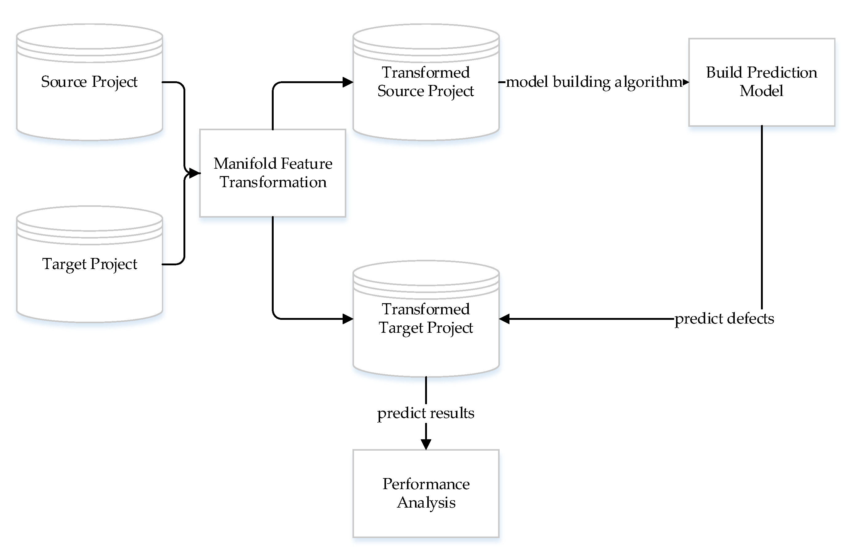
3.2. Method Framework

The framework of the MFTCPDP method is shown in Figure 1. The input is a source project and a target project. After manifold feature transformation, new source projects and target projects were obtained. Then, we used the machine learning model to build a defect prediction model on the transformed source project and predict defects on the transformed target project to obtain a prediction label. Finally, the performance of the MFTCPDP method was compared with real labels. The core of the MFTCPDP method lies in the process of manifold feature transformation. We introduce the concept and implementation details of manifold feature transformation in the next section.

3.3. Manifold Feature Transformation

Manifold feature transformation is to transform the original feature space into manifold space and then reduce the data distribution difference between the transformed source project and the transformed target project in the manifold space. The data in the manifold space have the low-dimensional manifold structure of high-dimensional space. Therefore, the data features have good geometric properties, which can avoid the phenomenon of feature distortion [36]. Therefore, we first transformed the features in the original space into the manifold space and then transferred them in the manifold space.

In the Grassmann manifold, the feature transformation has an effective numerical form, which can be expressed and solved efficiently [37]. Therefore, this paper transformed the original feature space into the Grassmann manifold space. There are many ways to accomplish this process [38,39]. We chose the geodesic flow kernel method (i.e., GFK) [40,41] to complete the manifold feature transformation process because GFK has higher computational efficiency.

GFK attempts to model the data domain with d-dimensional subspaces and then embeds these subspaces into the manifold $G$. Let $P_s$ and $P_T$ respectively, represent the subspace of the original data space after principal component analysis, then $G$ can be regarded as a collection of all d-dimensional subspaces. Each d-dimensional original subspace can be regarded as a point on $G$. Therefore, the geodesic $\{\Phi (t),0\le t\le 1\}$ between two points can form a path between the two subspaces. If we make $P_S=\Phi (0),P_T=\Phi (1)$, then finding a geodesic from $\Phi (0)$ to $\Phi (1)$ is equivalent to transforming the original feature into an infinite-dimensional space, and the integral calculation of this path is the process of migrating the source project to the target project in the manifold space so as to reduce the data distribution difference between the two projects [36]. This method can be considered an incremental migration method from $\Phi (0)$ to $\Phi (1)$. Below, we will introduce the construction process and solution process in detail.

$P_s\in {ℝ}^{D\times d}$ and $P_T\in {ℝ}^{D\times d}$ respectively represent the subspace of the source project dataset and the target project dataset after principal component analysis, and d represents the feature dimension of the subspace, $R_s\in {ℝ}^{(D-d)\times d}$ represents the orthogonal complement to $P_s$. Using the canonical Euclidean metric of the Riemannian manifold, the geodesic flow is parameterized [38] as follows:

$$\Phi (t)\in G(d,D),t\in [0,1]$$

Additionally, $P_s=\Phi (0),P_T=\Phi (1)$, for the other t:

$$\Phi (t)=P_s{U}_1\Gamma (t)-R_s{U}_2\Sigma (t)$$

where $U_1\in {ℝ}^{d\times d},U_2\in {ℝ}^{(D-d)\times d}$ are orthogonal matrices, and they are given by the following SVDs:

$$P_s^T{P}_T=U_1\Gamma V^T,R_s^T{P}_T=-U_2\Sigma V^T$$

where $\Gamma$ and $\Sigma$ are diagonal matrices. The diagonal elements are $\cos {\theta }_i$ and $\sin {\theta }_i$, i = 1,2,…,d. ${\theta }_i$ represents the principal angles between $P_s$ and $P_T$.

$$0\le {\theta }_1\le {\theta }_2\le \dots \le {\theta }_d\le \pi /2$$

For the two original feature vectors $F_i$ and $F_j$, we compute their projections into Φ(t) for a continuous t from 0 to 1 and concatenate all the projections into infinite-dimensional feature vectors ${{\rm Z}}_i^{\infty }$ and ${{\rm Z}}_j^{\infty }$. The inner product [40] between them defines our geodesic-flow kernel as follows:

$$〈{{\rm Z}}_i^{\infty },{{\rm Z}}_j^{\infty }〉={\displaystyle {\int }_0^1(\Phi {(t)}^T{F}_i)(\Phi {(t)}^T{F}_j)}dt=F_i{}^{T}G{F}_j$$

Therefore, through ${\rm Z}=\sqrt{G}F$, the features in the original space can be transformed into the Grassmann manifold space and the migration from the source project to the target project can be completed.

$G$ is a positive semidefinite matrix, which can be computed [41] in a closed-form from previously defined matrices as follows:

$$G=\left[P_s\right.U_1\left.R_s{U}_2\right]\left(\begin{array}{cc}{\Lambda }_1& {\Lambda }_2\\ {\Lambda }_2& {\Lambda }_3\end{array}\right)\left(\begin{array}{cc}{U}_1^T& P_s^T\\ U_2^T& R_s^T\end{array}\right)$$

where ${\Lambda }_1,{\Lambda }_2,{\Lambda }_3$ are diagonal matrices, whose diagonal elements are

$${\lambda }_{1i}=1+\frac{\sin 2{\theta }_i}{2{\theta }_i},{\lambda }_{2i}=1+\frac{\cos 2{\theta }_i-1}{2{\theta }_i},{\lambda }_{3i}=1-\frac{\sin 2{\theta }_i}{2{\theta }_i}$$

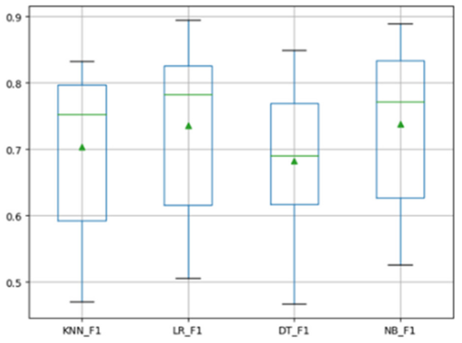
3.4. Model Building Algorithm

According to the above process, the model construction algorithm is shown as follows (Algorithm 1):

Algorithm 1 MFTCPDP

Input: Labeled Source Project S, Unlabeled Target Project T Output: Predicted labels L

1: Preprocess the project data to get SP and TP;

2: Construct the manifold space according to Equations (1)–(3);

3: Calculate G according to Equations (5)–(7);

4: Use G to perform a manifold transformation on SP and TP and get SG, TG;

5: Use SG to train naive Bayes classifier and predict the labels of TG;

6: loop all projects.

4. Experimental Research

This section explains the experimental research process to explore the experimental performance of the MFTCPDP method. We first introduce the experimental datasets and performance evaluation indicators used in the experiment, then set the parameters involved in the experiment, and finally analyze the experimental results.

4.1. Experimental Datasets

The Relink dataset [42] and the AEEEM dataset [43] are two open source datasets that are frequently used by researchers in the field of software defect prediction. We also used these two datasets in our experiments.

Table 1. Experimental datasets.

Project	Modules	Features	Defects	Defect Ratio
Apache	194	26	98	50%
Safe	56	26	22	39%
ZXing	399	26	118	30%
EQ	325	61	129	40%
JDT	997	61	206	21%
LC	399	61	64	9%
ML	1862	61	245	13%
PDE	1492	61	209	14%

shows the project name, the number of modules, the number of features, the number of defects, and the defect ratio of the two datasets [44]. Among them, Apache, Safe, and ZXing belong to the Relink dataset, and the rest are projects in the AEEEM dataset.

From Table 1, we can observe that the projects in the Relink dataset have 26 features, and the projects in the AEEEM dataset have 61 features. The research of this paper aimed to carry out experimental exploration on the phenomenon of feature distortion when there are many features and put forward the solution of manifold feature transformation.

The features of the two datasets are mainly described from code complexity and abstract syntax tree. The Understand website (https://www.scitools.com, accessed on 18 August 2021) can query the specific meaning of each feature.

4.2. Evaluation Indicator

This paper focuses on the two classifications of software defects—that is, whether the classification result is defective or not. There are some two-category evaluation indicators in research related to machine learning, such as accuracy, precision, and recall.

$$\mathrm{F}1=\frac{2*Precision*Recall}{Precision+Recall}$$

Among these indicators, researchers in the field of software defect prediction often use the F1 value. From the actual situation of the software project, only a few software modules may have defects. If only the accuracy indicator is used to evaluate, even if all modules are judged to be free of defects, the accuracy value will be very high, but this does not mean that the effect of the model is better. It can be inferred from Equation (8) that the F1 value is the harmonic average of precision and recall indicators, and the values of these two indicators are considered at the same time. Therefore, we also used the F1 value as the main evaluation indicator.

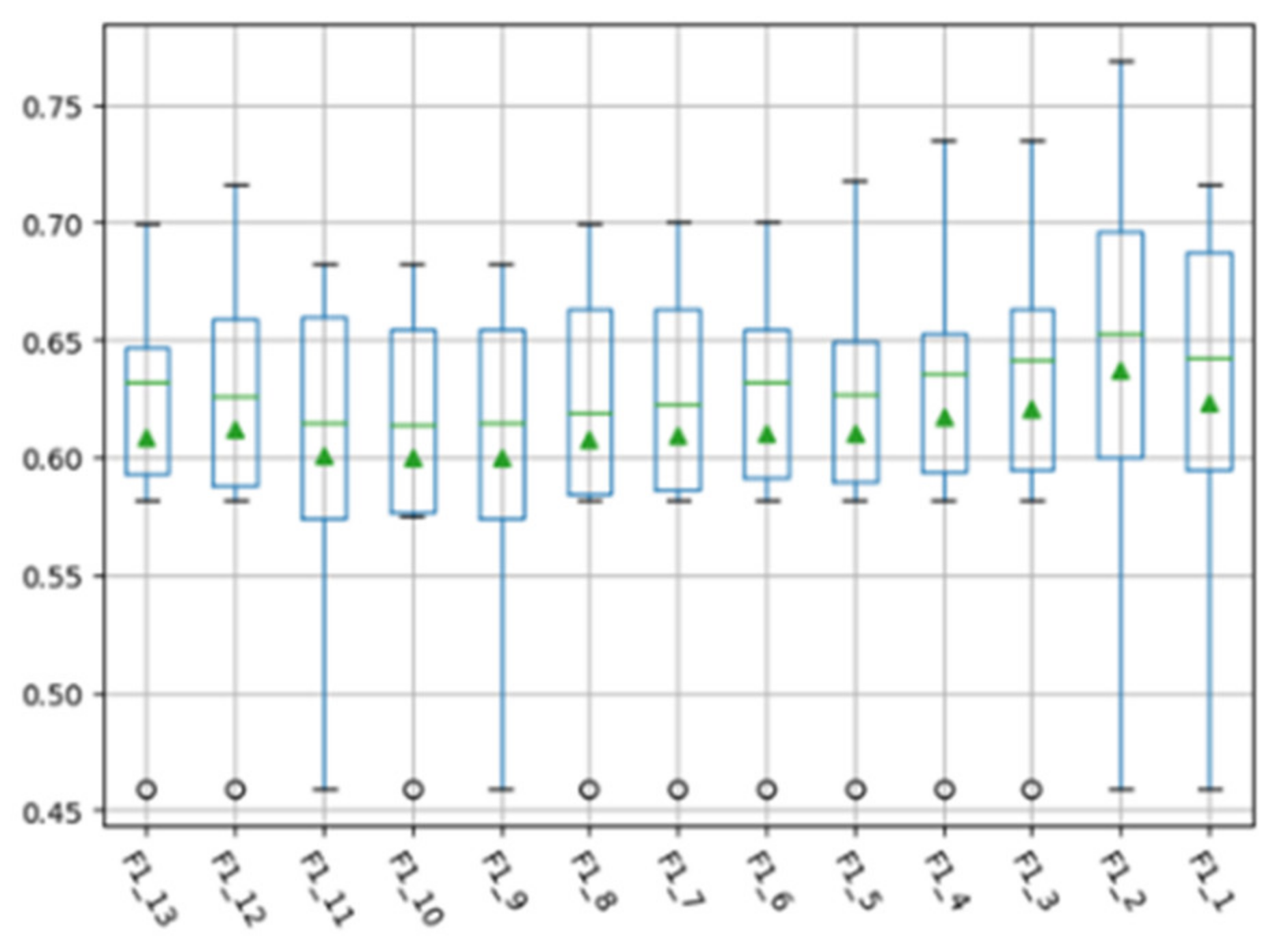
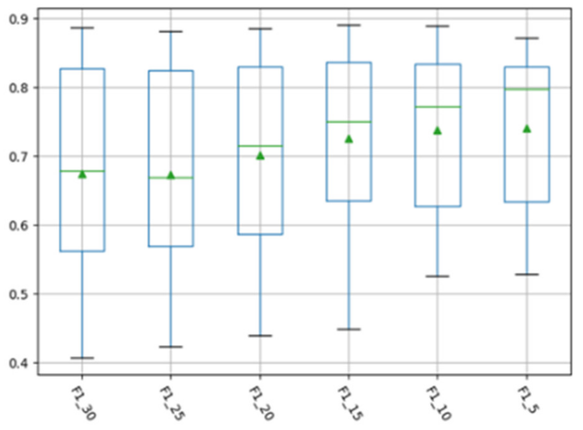
4.3. Experimental Parameter Setting

The MFTCPDP method mainly includes two main steps—manifold feature transformation and defect prediction model construction. In the process of manifold feature transformation, we need to set the feature dimension. For the Relink dataset, we set the feature dimension as 2, and for the AEEEM dataset, we set the feature dimension as 10. In the experiment, we chose the naive Bayes classifier as the default classifier when building the model. The influence of different feature dimensions and different classifiers on the MFTCPDP method are discussed below.

All experiments were run on a computer with the following configuration: Windows 10, 64-bit; CPU: Intel(R) Core(TM) i5-6300HQ [email protected]; RAM: 12G.

4.4. Experimental Results and Analysis

In order to verify the effectiveness of the MFTCPDP method, we first conducted an experimental study on the MFTCPDP method on two datasets frequently used by researchers, then compared the performance with the benchmark method, several currently popular CPDP methods and WPDP methods. Finally, we considered the internal factors that affect the performance of the MNTCPDP method, including the influence of the method parameters and the choice of a classifier on the method performance. Therefore, we designed three research questions and realized a comprehensive analysis of the MFTCPDP method through the answers to these questions.

Question 1: Compared with the benchmark method, can the MFTCPDP method improve the performance of CPDP? Additionally, is it better than several popular CPDP methods? How does the performance compare to the WPDP method?

Herbold et al. [45] and Zhou et al. [46] conducted empirical studies on the current reproducible CPDP methods and found that most of the current CPDP methods are difficult to surpass the performance of some existing classical methods, such as the method of reducing distribution difference proposed by Watanabe et al. [47] evaluated by Herbold et al., the Burak filtering method based on instance selection proposed by TURHAN et al. [14], and the TCA + method based on feature transformation and migration proposed by Nam et al. [19]. These three methods rank high in the comprehensive performance of all CPDP methods; therefore, we compared the MFTCPDP method with these three CPDP methods. Moreover, in the CPDP research, Zimmermann et al. [26] proposed a method of directly using source project data to train the model and then predicting the target project, which is recorded as the DCPDP (i.e., direct cross-project defect prediction) method. It is often used as a benchmark method for comparison. In addition, we have also conducted an experimental comparison with the 10-fold cross-validated WPDP method. The 10-fold cross-validated WPDP method is the most reasonable experimental setting, which can show the gap between the MFTCPDP method and WPDP and analyze the problems of the current method.

Before the performance comparison of the methods, we first conducted experiments to explore the feature distortion phenomenon in the original feature space. Therefore, we carried out the experiment of the DCPDP method with data standardization operation, which was recorded as the comparison between the DCPDP-Norm and the DCPDP method. Generally speaking, a simple data normalization operation can improve the experimental performance, but when the value distribution in the feature space is distorted, the experimental performance may be reduced.

We conducted experiments on two datasets and obtained the following experimental results.

Table 2. Comparison of F1 values between DCPDP-Norm and DCPDP.

Source→Target	DCPDP-Norm	DCPDP
Apache→Safe	0.787	0.459
Apache→ZXing	0.606	0.582
Safe→Apache	0.583	0.714
Safe→ZXing	0.651	0.654
ZXing→Apache	0.437	0.645
ZXing→Safe	0.645	0.699
EQ→JDT	0.596	0.422
EQ→LC	0.843	0.813
EQ→ML	0.367	0.344
EQ→PDE	0.775	0.687
JDT→EQ	0.716	0.633
JDT→LC	0.755	0.884
JDT→ML	0.788	0.769
JDT→PDE	0.702	0.826
LC→EQ	0.709	0.663
LC→JDT	0.804	0.545
LC→ML	0.770	0.462
LC→PDE	0.771	0.789
ML→EQ	0.711	0.688
ML→JDT	0.732	0.578
ML→LC	0.837	0.875
EQ→JDT	0.804	0.809
EQ→LC	0.722	0.674
EQ→ML	0.519	0.571
EQ→PDE	0.523	0.871
JDT→EQ	0.384	0.437

shows the performance comparison between DCPDP-Norm and DCPDP.

Table 3. Comparison of F1 value between MFTCPDP and several CPDP methods and WPDP.

Source→Target	MFTCPDP	TCA+	Watanabe	Burak	DCPDP	WPDP
Safe→Apache	0.711	0.670	0.716	0.565	0.714	0.625
ZXing→Apache	0.653	0.671	0.705	0.358	0.645
ZXing→Safe	0.769	0.512	0.717	0.735	0.699	0.703
Apache→Safe	0.460	0.569	0.717	0.234	0.459
Apache→ZXing	0.587	0.595	0.653	0.155	0.582	0.666
Safe→ZXing	0.652	0.628	0.636	0.596	0.654
MEAN	0.638	0.607	0.691	0.441	0.625	0.665
JDT→EQ	0.556	0.606	0.688	0.452	0.633	0.723
LC→EQ	0.667	0.549	0.683	0.473	0.663
ML→EQ	0.623	0.637	0.679	0.452	0.688
PDE→EQ	0.628	0.608	0.687	0.453	0.674
LC→JDT	0.572	0.731	0.818	0.700	0.545	0.829
PDE→JDT	0.724	0.743	0.827	0.702	0.571
ML→JDT	0.608	0.726	0.828	0.701	0.578
EQ→JDT	0.527	0.455	0.736	0.432	0.422
JDT→LC	0.889	0.798	0.825	0.861	0.884	0.865
ML→LC	0.882	0.861	0.860	0.863	0.875
PDE→LC	0.876	0.786	0.811	0.860	0.871
EQ→LC	0.842	0.479	0.015	0.808	0.813
JDT→ML	0.836	0.772	0.777	0.805	0.769	0.837
LC→ML	0.781	0.470	0.806	0.807	0.462
PDE→ML	0.833	0.788	0.807	0.807	0.437
EQ→ML	0.762	0.385	0.349	0.590	0.344
EQ→PDE	0.718	0.619	0.760	0.525	0.687	0.831
JDT→PDE	0.828	0.797	0.781	0.790	0.826
LC→PDE	0.780	0.804	0.812	0.796	0.789
ML→PDE	0.822	0.819	0.822	0.794	0.809
MEAN	0.738	0.671	0.718	0.684	0.667	0.817

shows the performance comparison between the MFTCPDP method and benchmark method DCPDP, several DCPDP methods, and WPDP method.

First, we compared DCPDP and DCPDP-Norm with data standardization operations. As shown in Table 2, the overall performance difference between the DCPDP-Norm and the DCPDP on the Relink dataset (i.e., rows 2 to 7) is considerably noticeable. Specifically, it can be found in each pair of CPDP experiments that data standardization operation sometimes cannot improve the performance of the method or even regress the performance. In Relink dataset, the performance of four pairs of experiments decreased significantly using the DCPDP-Norm method; in the cases in which the performance decreased significantly, such as in the Safe→Apache pair, the F1 value of DCPDP was 0.714, but the F1 value of DCPDP-Norm was 0.583. Among the six experiments on Relink dataset, only two sets of experiments have improved the performance of data standardization operations. There is also such a phenomenon on the AEEEM dataset (i.e., rows 8 to 27). For example, JDT→LC, JDT→PDE, and PDE→ML are all reduced in performance after data standardization operations. Generally speaking, on the two datasets, performance degradation is not rare. There are 26 groups of CPDP experiments in total, and 12 groups have performance degradation. Almost half of the experimental performances have not been improved. However, under normal circumstances, using the data after the data standardization operation to train the model can often obtain better performance. Therefore, we believe that there is a feature distortion phenomenon in the data distribution of the original feature space, which causes a decrease in the performance level of the experiment, rather than an increase.

Table 3 shows the performance comparison between the MFTCPDP method and the benchmark method DCPDP, several CPDP methods, and the WPDP method. Firstly, compared with DCPDP, in a total of 26 CPDP experiments on the two datasets, the MFTCPDP method can achieve better prediction performance in most of the cross-project defect prediction experiments. The F1 value of the MFTCPDP method is higher in 20 groups of experiments, and the F1 value of the remaining 6 groups of experiments is higher in the DCPDP method, but the performance gap of these 6 groups of experiments is very weak. For example, in the Safe→ZXing experiment, MFTCPDP obtained an F1 value of 0.652, while DCPDP obtained an F1 value of 0.654, with a difference of only 0.002. From the average value, the performance of MFTCPDP is also better. The DCPDP method achieved an average value of 0.625 on the Relink dataset and an average value of 0.667 on the AEEEM dataset, while the MFTCPDP method obtained an average value of 0.638 on Relink dataset and 0.738 on the AEEEM dataset. In addition, from the distribution of performance values, the minimum F1 value obtained by the DCPDP method in all experiments is 0.344, the maximum F1 value is 0.884, and there are five groups of experiments with a value lower than 0.5, but the minimum F1 value obtained by MFTCPDP method in all experiments is 0.460, the maximum F1 value is 0.889, and only one group of experiments with a value lower than 0.5. This shows that the MFTCPDP method has a smaller F1 value fluctuation range than the DCPDP method, and the overall performance is more stable. Therefore, compared with the benchmark method DCPDP, the MFTCPDP method can improve the performance of CPDP.

Compared with several CPDP methods, the MFTCPDP method also has advantages. Compared with the Burak filter method, the MFTCPDP method achieved better performance in all CPDP experiments on the Relink dataset. At the same time, MFTCPDP also performed better in average performance. The Burak filter method achieved an average performance value of 0.441, while the MFTCPDP method achieved an average performance value of 0.638. In the 20 groups of CPDP experiments on the AEEEM dataset, the MFTCPDP method performed better in 16 groups. In the other 4 groups of experiments, although the performance was not as high as the Burak filter method, the gap is also very small. For example, in the two experiments of LC→ML and LC→PDE, the performance values of the two are basically around 0.8. From the perspective of performance stability, the Burak filter method has the lowest performance on the Relink dataset of 0.155 and the highest value of 0.735. The lowest performance on the AEEEM dataset is 0.432, the highest value is 0.863, and the performance fluctuates greatly, while the performance of the MFTCPDP method is relatively stable without a significant difference in performance. In fact, the Burak filter method is an instance selection method based on similarity, which simply relies on similarity measurement and destroys the distribution of datasets. Therefore, in many cases, the performance of the Burak filter method fluctuates greatly, and the performance is not ideal. From this perspective, the MFTCPDP method has more advantages. Compared with TCA+, our method MFTCPDP also performs better. In the six sets of experiments on the Relink dataset, three sets of MFTCPDP methods performed better. Among the 20 sets of experiments on the AEEEM dataset, 13 sets of MFTCPDP methods performed better. In terms of average value, the MFTCPDP method achieved the average performance of 0.638 and 0.738, respectively, while TCA+ only obtained average performance of 0.607 and 0.671. In general, the MFTCPDP method is indeed better than TCA+. As we discussed earlier, feature distortion is easy to occur when there are many features in the dataset, and the TCA+ method is to map the data of the source project and the target project into a potential space to reduce the distribution difference between the source project and the target project. In the case of feature distortion, TCA+ may not be able to map to the latent space while preserving the structure and features of the original dataset. Therefore, the performance is not ideal in many cases. Compared with the Watanabe method, the MFTCPDP method also has advantages, but the advantages are relatively weak. In terms of average performance, on the Relink dataset, the MFTCPDP method achieved an average performance of 0.638, while the Watanabe method achieved an average performance of 0.691. On the AEEEM dataset, the average performance of the MFTCPDP method reached 0.738, while the Watanabe method achieved an average performance of 0.718. From this point of view, there seems to be little difference. However, the Watanabe method performs abnormally in some cases. For example, the F1 value of EQ→LC is only 0.015, and the F1 value of EQ→ML is only 0.349. We analyzed that the Watanabe method relies on the mean value of the attribute to reduce the distribution difference of the data. Sometimes, the value of some attributes is special, such as when the value is all 0, the average value of the attribute is 0, etc., resulting in poor performance in some cases. Therefore, some feature selection methods need to be combined with the Watanabe method to achieve better performance.

Finally, we compared the performance of the MFTCPDP method and the 10-fold cross-validated WPDP. Since WPDP uses part of the project data to train the model to predict the remaining part of the data, only one F1 value was generated for each project. It can be inferred from Table 3 that our MFTCPDP method has a large gap, compared with WPDP. Only in the experiment with Apache as the target project, the performance of MFTCPDP completely exceeds WPDP. Additionally, in the experiment with LC as the target project, three groups of experiments of MFTCPDP surpass WPDP. However, the performance of other experiments is completely inferior to WPDP. The same is true for the other CPDP methods, and it is difficult to surpass the WPDP method. However, the WPDP method is not suitable for practical applications. Therefore, this is also the focus of current CPDP research. When the target project is completely unmarked, the performance of CPDP should further improve so as to be used in actual production.

In order to ensure that our analysis is reasonable, we carried out a statistical test and analysis on the above experimental results. We used Wilcoxon signed-rank test, which is a non-parametric statistical hypothesis test used to judge whether two matched samples are selected from the same distribution. If the p-value reported by the Wilcoxon signed-rank test is less than 0.05, then the distributions to be tested are considered to be significantly different; otherwise, they are not considered to be significant.

We conducted four groups of Wilcoxon signed-rank tests—namely, MFTCPDP and TCA+, MFTCPDP and Burak, MFTCPDP and DCPDP, MFTCPDP and Watanabe, respectively marked as M&T, M&B, M&D, and M&W. Finally, we obtained four p values—namely, M&T 0.0248, M&B 0.0002, M&D 0.004, and M&W 0.2796. We found that the p values of M&T, M&B, and M&D are all less than 0.05, which means that there is a significant difference between MFTCPDP and TCA+, Burak, DCPDP. This shows that our above analysis is reasonable. Additionally, compared with the benchmark method DCPDP, the CPDP method Burak filter, and the TCA+, our MFTCPDP method indeed performs better. However, the p value of M&W is 0.2796, which exceeds 0.05. This shows that there is no significant difference between MFTCPDP and Watanabe. However, this does not mean that our above analysis is unreasonable. In fact, in terms of overall performance, compared with Watanabe, the advantage of MFTCPDP is indeed very weak, but the Watanabe method performed abnormally in some cases mentioned above. Therefore, our MFTCPDP method is more reliable from this point of view.

Finally, we explain the execution efficiency of the MFTCPDP algorithm (i.e., Algorithm 1). The 26 groups of experiments shown in Table 3 are all executed by the process shown in Algorithm 1. We executed the algorithm twice. The first time we executed it on the Relink dataset, we obtained six sets of experimental results, which required about 3.2 s; the second time we executed it on the AEEEM dataset, we obtained 20 sets of experimental results, which required about 10.8 s. The average time of each experiment is about 0.5 s. This time efficiency is acceptable.

Question 2: How does the setting of different subspace dimensions in the MFTCPDP method affect the performance of the method?

In the manifold feature transformation of source project and target project, the selection of subspace dimension entails how many dimensions of data need to be retained to represent the source project and the target project in the manifold space. This parameter may have an impact on the experimental performance. We aimed to analyze whether different dimension settings affect the final experimental performance, and then confirm the optimal subspace dimension. In order to analyze the influence of setting different subspace dimensions on the performance of the MFTCPDP method during the transformation of manifold features, we selected different subspace dimensions on the Relink dataset and the AEEEM dataset to conduct experiments. The software projects on Relink dataset have 26 features; therefore, we selected subspace dimensions from 13 to 1 for experiments. The software projects on the AEEEM dataset have 61 features, and the number of features is relatively large; therefore, we studied the performance in several subspace dimensions of 30, 25, 20, 15, 10, and 5. We made box plots of F1 values corresponding to different subspace dimensions for all CPDP experiments on the Relink dataset and AEEEM dataset, as shown in Figure 2 and Figure 3 below.

In the figures, the horizontal axis represents the observed indicator and the selected feature dimension, and the vertical axis represents the corresponding indicator value. For example, F1_13 in Figure 2 represents the F1 indicator value with 13 subspace dimensions of the Relink dataset.

As can be observed from Figure 2, with the decrease in the subspace dimension on the Relink dataset, the F1 value obtained by the MFTCPDP method gradually increases, and the maximum value of the F1 indicator and the overall value distribution slowly increase. It reaches the maximum value when the subspace dimension is 2, and the performance suddenly decreases when the subspace dimension is 1. The minimum values of each group of experiments are very close, and they are all at the lowest point of the box plot. Therefore, we deduce that on the Relink dataset, the selection of the subspace dimension has a certain impact on the experimental performance, and the performance is best when the subspace dimension is 2. It can be observed from Figure 3 that the performance of the F1 value on the AEEEM dataset is similar to that of Figure 2. Basically, as the subspace dimension decreases, the F1 value obtained by the MFTCPDP method gradually increases, but the improvement here is more obvious. Both the minimum value and overall value distribution are improved, and the performance decreases when the last subspace dimension is 5. Therefore, we also deduce that on the AEEEM dataset, the selection of the subspace dimension has a certain impact on the experimental performance, and the performance is best when the subspace dimension is 10.

Analyzing the above two figures, we conclude that the selection of the subspace dimension in the manifold feature transformation will have a certain impact on the experimental performance of the method. Choosing an appropriate subspace dimension can achieve better experimental performance.

Question 3: How do different classification models affect the performance of the MFTCPDP method?

Any method requires a classifier to complete the construction of the defect prediction model, and the MFTCPDP method is no exception. In the field of software defect prediction, different types of classifiers may have uncertain effects on the final experimental performance. Therefore, we need to study the impact of different classifiers on the performance of the MFTCPDP method. In response to this problem, we selected several different types of classification models. We compared the experimental results of decision tree (DT), logistic regression (LR), k-nearest neighbor (KNN), and naive Bayes (NB). We made the F1 values of all cross-project defect prediction experiments on the Relink dataset and the AEEEM dataset into box plots. Figure 4 and Figure 5 show the F1 values obtained by the MFTCPDP method using different classifiers.

The horizontal axis in the figures represents the classifiers and indicators used. For example, KNN_F1 represents the F1 value obtained by the MFTCPDP method using the KNN classifier in the experiment, and the vertical axis represents the corresponding F1 value.

As can be observed from Figure 4, in the Relink dataset, the F1 values of all classifiers are not significantly different, and the performance of the naive Bayes classifier is slightly better. Figure 5 reveals that in the AEEEM dataset, all classifiers perform very similarly in F1 values. Only the F1 value of the decision tree model is more stable above 0.6, the values of the other three classifiers are slightly scattered. However, the performance of the decision tree model on the Relink dataset is general; therefore, we chose the naive Bayes classifier in this paper.

Through the above analysis, we can draw the conclusion that among the several classification models experimented with the MFTCPDP method, the overall performance of the naive Bayes classifier is relatively better. Different types of classification models will have a certain impact on the performance of the MFTCPDP method. Choosing a suitable model for different methods can improve the performance of CPDP.

5. Conclusions and Prospects

This paper proposed a cross-project defect prediction method based on manifold feature transformation, which can avoid feature distortion in the original feature space and effectively reduce the difference in data distribution between the source project and the target project in the manifold space. Experimental research shows that our method can alleviate the feature distortion in the original feature space, and especially when the feature dimension is large, it can improve the performance of cross-project defect prediction.

A question worth discussing is why our method achieves better performance, especially when compared with the feature transformation and migration methods such as TCA+. As the results of previous experiments have shown, performing feature transformation and migration in the original feature space may not be able to capture the potential public space. It is more suitable for transformation and migration in the manifold space when the data feature dimension is high. Therefore, our method of manifold feature transformation is more effective in this case.

At present, some artificial intelligence algorithms and their applications are also developing very rapidly, such as online learning algorithms [48], multi-objective optimization algorithms [49], related heuristic algorithms [50], etc. Therefore, CPDP research does not stop at using the feature transformation or feature migration methods mentioned in this article. The above is also worthy of being introduced into different scenarios of CPDP research. For example, online learning algorithms are combined with just-in-time software defect prediction [51], training models are obtained through dynamic incremental methods, multi-objective optimization and some heuristic algorithms are used for feature selection and instance selection [52], some data classification algorithms are used to enhance the effectiveness of defect prediction [53], etc.

There are still many future steps worth noting in this paper. Firstly, the feature dimension of the original feature space transformed to the manifold space was not automatically selected. The later stage can focus on the automatic selection of the optimal parameters. Secondly, the distribution difference between the source project and the target project in the manifold space can be adapted from two aspects—edge distribution and conditional distribution, which were not considered in this paper. Thirdly, in the experiment, we chose two datasets of software projects, and our method can further extend to other suitable datasets in later periods. Finally, different classifiers have a certain impact on the method, and relevant research shows that ensemble learning can significantly improve the performance of the method. In the future, we can study the impact of ensemble learning on the performance of the cross-project defect prediction method.

References

1. Gong, L.N.; Jiang, S.J.; Jiang, L. Research progress of software defect prediction. J. Softw. 2019, 30, 3090–3114. [Google Scholar]
2. Chen, X.; Gu, Q.; Liu, W.S.; Liu, S.; Ni, C. Survey of static software defect prediction. J. Softw. 2016, 27, 1–25. [Google Scholar]
3. Tracy, H.; Sarah, B.; David, B.; Gray, D.; Counsell, S. A systematic literature review on fault prediction performance. IEEE Trans. Softw. Eng. 2012, 38, 1276–1304. [Google Scholar]
4. Li, Z.; Jing, X.Y.; Zhu, X. Progress on approaches to software defect prediction. IET Softw. 2018, 12, 161–175. [Google Scholar] [CrossRef]
5. Li, Y.; Huang, Z.Q.; Wang, Y.; Fang, B.W. Survey on data driven software defects prediction. Acta Electron. Sin. 2017, 45, 982–988. [Google Scholar]
6. Chidamber, S.R.; Kemerer, C.F. A metrics suite for object-oriented design. IEEE Trans. Softw. Eng. 1994, 20, 476–493. [Google Scholar] [CrossRef] [Green Version]
7. Jin, C. Software defect prediction model based on distance metric learning. Soft Comput. 2021, 25, 447–461. [Google Scholar] [CrossRef]
8. Hosseini, S.; Turhan, B.; Gunarathna, D. A systematic literature review and meta-analysis on cross project defect prediction. IEEE Trans. Softw. Eng. 2019, 45, 111–147. [Google Scholar] [CrossRef] [Green Version]
9. Bowes, D.; Hall, T.; Petric, J. Software defect prediction: Do different classifiers find the same defects. Softw. Qual. J. 2018, 26, 525–552. [Google Scholar] [CrossRef] [Green Version]
10. Manjula, C.; Florence, L. Deep neural network-based hybrid approach for software defect prediction using software metrics. Clust. Comput. 2019, 22, 9847–9863. [Google Scholar] [CrossRef]
11. Chen, S.; Ye, J.M.; Liu, T. Domain adaptation approach for cross-project software defect prediction. J. Softw. 2020, 31, 266–281. [Google Scholar]
12. Chen, X.; Wang, L.P.; Gu, Q.; Wang, Z.; Ni, C.; Liu, W.S.; Wang, Q. A survey on cross-project software defect prediction methods. Chin. J. Comput. 2018, 41, 254–274. [Google Scholar]
13. Herbold, S.; Trautsch, A.; Grabowski, J. Global vs. local models for cross-project defect prediction. Empir. Softw. Eng. 2017, 22, 1866–1902. [Google Scholar] [CrossRef]
14. Turhan, B.; Menzies, T.; Bener, A.; Di Stefano, J. On the relative value of cross-company and within-company data for defect prediction. Empir. Softw. Eng. 2009, 14, 540–578. [Google Scholar] [CrossRef] [Green Version]
15. Peters, F.; Menzies, T.; Marcus, A. Better cross company defect prediction. In Proceedings of the 2013 10th Working Conference on Mining Software Repositories, San Francisco, CA, USA, 18–19 May 2013; IEEE: Piscataway, NJ, USA, 2013; pp. 409–418. [Google Scholar]
16. Ying, M.; Luo, G.; Xue, Z.; Chen, A. Transfer learning for cross-company software defect prediction. Inf. Softw. Technol. 2012, 54, 248–256. [Google Scholar]
17. Xia, X.; Lo, D.; Pan, S.J.; Nagappan, N.; Wang, X. Hydra: Massively compositional model for cross-project defect prediction. IEEE Trans. Softw. Eng. 2016, 42, 977–998. [Google Scholar] [CrossRef]
18. Sun, Z.; Li, J.; Sun, H.; He, L. CFPS: Collaborative filtering based source projects selection for cross-project defect prediction. Appl. Soft Comput. 2020, 99, 106940. [Google Scholar]
19. Nam, J.; Pan, S.J.; Kim, S. Transfer defect learning. In Proceedings of the 2013 35th International Conference on Software Engineering, San Francisco, CA, USA, 18–26 May 2013; IEEE: Piscataway, NJ, USA, 2013; pp. 382–391. [Google Scholar]
20. Yu, Q.; Jiang, S.; Zhang, Y. A feature matching and transfer approach for cross-company defect prediction. J. Syst. Softw. 2017, 132, 366–378. [Google Scholar] [CrossRef]
21. Ni, C.; Chen, X.; Liu, W.S. Cross-project defect prediction method based on feature transfer and instance transfer. J. Softw. 2019, 30, 1308–1329. [Google Scholar]
22. Wang, J.; Chen, Y.; Hao, S.; Feng, W.; Shen, Z. Balanced distribution adaptation for transfer learning. In Proceedings of the 2017 IEEE International Conference on Data Mining, New Orleans, LA, USA, 18–21 November 2017; IEEE: Piscataway, NJ, USA, 2017; pp. 1129–1134. [Google Scholar]
23. Wang, J.; Feng, W.; Chen, Y.; Yu, H.; Huang, M.; Yu, P.S. Visual domain adaptation with manifold embedded distribution alignment. In Proceedings of the 26th ACM International Conference on Multimedia, New York, NY, USA, 22–26 October 2018; ACM: New York, NY, USA, 2018; pp. 402–410. [Google Scholar]
24. Baktashmotlagh, M.; Harandi, M.T.; Lovell, B.C.; Salzmann, M. Unsupervised domain adaptation by domain invariant projection. In Proceedings of the IEEE International Conference on Computer Vision. Sydney Convention and Exhibition Centre, Sydney, Australia, 1–8 December 2013; ACM: New York, NY, USA, 2013; pp. 769–776. [Google Scholar]
25. Briand, L.C.; Melo, W.L.; Wust, J. Assessing the applicability of fault-proneness models across object-oriented software projects. IEEE Trans. Softw. Eng. 2002, 28, 706–720. [Google Scholar] [CrossRef] [Green Version]
26. Zimmermann, T.; Nagappan, N.; Gall, H.; Giger, E.; Murphy, B. Cross-project defect prediction: A large scale experiment on data vs. domain vs. process. In Proceedings of the 7th Joint Meeting of the European Software Engineering Conference and the ACM Sigsoft Symposium on the Foundations of Software Engineering, New York, NY, USA, 24–28 August 2009; pp. 91–100. [Google Scholar]
27. He, Z.; Shu, F.; Yang, Y.; Li, M.; Wang, Q. An investigation on the feasibility of cross-project defect prediction. Autom. Softw. Eng. 2012, 19, 167–199. [Google Scholar] [CrossRef]
28. Herbold, S. Training data selection for cross-project defect prediction. In Proceedings of the 9th International Conference on Predictive Models in Software Engineering, New York, NY, USA, 9 October 2013; pp. 61–69. [Google Scholar]
29. Yu, Q.; Jiang, S.; Qian, J. Which is more important for cross-project defect prediction: Instance or feature. In Proceedings of the 2016 International Conference on Software Analysis, Testing and Evolution, Kunming, China, 3–4 November 2016; Volume 11, pp. 90–95. [Google Scholar]
30. Yu, Q.; Qian, J.; Jiang, S.; Wu, Z.; Zhang, G. An empirical study on the effectiveness of feature selection for cross-project defect prediction. IEEE Access 2019, 7, 35710–35718. [Google Scholar] [CrossRef]
31. Wu, F.; Jing, X.Y.; Sun, Y.; Sun, J.; Huang, L.; Cui, F. Cross-project and within-project semi supervised software defect prediction: A unified approach. IEEE Trans. Reliab. 2018, 67, 581–597. [Google Scholar] [CrossRef]
32. Li, Z.; Jing, X.Y.; Wu, F.; Zhu, X.; Xu, B.; Ying, S. Cost-sensitive transfer kernel canonical correlation analysis for heterogeneous defect prediction. Autom. Softw. Eng. 2018, 25, 201–245. [Google Scholar] [CrossRef]
33. Fan, G.; Diao, X.; Yu, H.; Chen, L. Cross-project defect prediction method based on instance filtering and transfer. Comput. Eng. 2020, 46, 197–202+209. [Google Scholar]
34. Zhang, Y.; Lo, D.; Xia, X.; Sun, J. An empirical study of classifier combination for cross-project defect prediction. In Proceedings of the IEEE Computer Software & Applications Conference, Taichung, Taiwan, 1–5 July 2015; Volume 7, pp. 264–269. [Google Scholar]
35. Chen, J.; Hu, K.; Yang, Y.; Liu, Y.; Xuan, Q. Collective transfer learning for defect prediction. Neurocomputing 2020, 416, 103–116. [Google Scholar] [CrossRef]
36. Balasubramanian, M.; Schwartz, E.L.; Tenenbaum, J.B.; de Silva, V.; Langford, J.C. The isomap algorithm and topological stability. Science 2002, 295, 7. [Google Scholar] [CrossRef] [PubMed] [Green Version]
37. Hamm, J.; Lee, D.D. Grassmann discriminant analysis: A unifying view on subspace-based learning. In Proceedings of the 25th International Conference on Machine Learning, New York, NY, USA, 5–9 July 2008; pp. 376–383. [Google Scholar]
38. Gopalan, R.; Li, R.; Chellappa, R. Domain adaptation for object recognition: An unsupervised approach. In Proceedings of the 2011 International Conference on Computer Vision, Barcelona, Spain, 6–13 November 2011; IEEE: Piscataway, NJ, USA, 2011; pp. 999–1006. [Google Scholar]
39. Baktashmotlagh, M.; Harandi, M.T.; Lovell, B.C.; Salzmann, M. Domain adaptation on the statistical manifold. In Proceedings of the IEEE Conference on Computer Vision and Pattern Recognition, Columbus, OH, USA, 23–28 June 2014; IEEE: Piscataway, NJ, USA, 2014; pp. 2481–2488. [Google Scholar]
40. Gong, B.; Shi, Y.; Sha, F.; Grauman, K. Geodesic flow kernel for unsupervised domain adaptation. In Proceedings of the IEEE Conference on Computer Vision and Pattern Recognition, Providence, RI, USA, 16–21 June 2012; IEEE: Piscataway, NJ, USA, 2012; pp. 2066–2073. [Google Scholar]
41. Wang, J.; Chen, Y.; Feng, W.; Yu, H.; Huang, M.; Yang, Q. Transfer learning with dynamic distribution adaptation. ACM Trans. Intell. Syst. Technol. 2020, 11, 1–25. [Google Scholar] [CrossRef] [Green Version]
42. Wu, R.; Zhang, H.; Kim, S.; Cheung, S.C. ReLink: Recovering links between bugs and changes. In Proceedings of the 19th ACM SIGSOFT Symposium and the 13th European Conference on Foundations of Software Engineering, Szeged, Hungary, 5–9 September 2011; ACM: New York, NY, USA, 2011; pp. 15–25. [Google Scholar]
43. Dambros, M.; Lanza, M.; Robbes, R. Evaluating defect prediction approaches: A benchmark and an extensive comparison. Empir. Softw. Eng. 2012, 17, 531–577. [Google Scholar] [CrossRef]
44. Yang, Y.; Yang, J.; Qian, H. Defect prediction by using cluster ensembles. In Proceedings of the 2018 Tenth International Conference on Advanced Computational Intelligence, Xiamen, China, 29–31 March 2018; IEEE: Piscataway, NJ, USA, 2018; pp. 631–636. [Google Scholar]
45. Steffen, H.; Alexander, T.; Jens, G. A comparative study to benchmark cross-project defect prediction approaches. IEEE Trans. Softw. Eng. 2017, 44, 811–833. [Google Scholar]
46. Zhou, Y.; Yang, Y.; Lu, H.; Chen, L.; Li, Y.; Zhao, Y.; Qian, J.; Xu, B. How far we have progressed in the journey? an examination of cross-project defect prediction. ACM Trans. Softw. Eng. Methodol. 2018, 27, 1–51. [Google Scholar] [CrossRef]
47. Watanabe, S.; Kaiya, H.; Kaijiri, K. Adapting a fault prediction model to allow inter language reuse. In Proceedings of the 4th International Workshop on Predictor Models in Software Engineering, Leipzig, Germany, 12–13 May 2008; IEEE: Piscataway, NJ, USA, 2008; pp. 19–24. [Google Scholar]
48. Zhao, H.; Zhang, C. An online-learning-based evolutionary many-objective algorithm. Inf. Sci. 2020, 509, 1–21. [Google Scholar] [CrossRef]
49. Liu, Z.Z.; Wang, Y.; Huang, P.Q. A many-objective evolutionary algorithm with angle-based selection and shift-based density estimation. Inf. Sci. 2020, 509, 400–419. [Google Scholar] [CrossRef] [Green Version]
50. Dulebenets, M.A. A novel memetic algorithm with a deterministic parameter control for efficient berth scheduling at marine container terminals. Marit. Bus. Rev. 2017, 2, 302–330. [Google Scholar] [CrossRef] [Green Version]
51. Pasha, J.; Dulebenets, M.A.; Kavoosi, M.; Abioye, O.F.; Wang, H.; Guo, W. An optimization model and solution algorithms for the vehicle routing problem with a “factory-in-a-box”. IEEE Access 2020, 8, 134743–134763. [Google Scholar] [CrossRef]
52. D’angelo, G.; Pilla, R.; Tascini, C.; Rampone, S. A proposal for distinguishing between bacterial and viral meningitis using genetic programming and decision trees. Soft Comput. 2019, 23, 11775–11791. [Google Scholar] [CrossRef]
53. Panda, N.; Majhi, S.K. How effective is the salp swarm algorithm in data classification. In Computational Intelligence in Pattern Recognition; Springer: Singapore, 2020; pp. 579–588. [Google Scholar]
Figure 1. MFTCPDP method framework.
Futureinternet 13 00216 g001
Figure 2. F1 values obtained from different subspace dimensions on the Relink dataset.
Futureinternet 13 00216 g002
Figure 3. F1 values obtained from different subspace dimensions on the AEEEM dataset.
Futureinternet 13 00216 g003
Figure 4. F1 values obtained by different classifiers on the Relink dataset.
Futureinternet 13 00216 g004
Figure 5. F1 values obtained by different classifiers on the AEEEM dataset.
Futureinternet 13 00216 g005