iCaps-Dfake: An Integrated Capsule-Based Model for Deepfake Image and Video Detection

Abstract

Fake media is spreading like wildfire all over the internet as a result of the great advancement in deepfake creation tools and the huge interest researchers and corporations are showing to explore its limits. Now anyone can create manipulated unethical media forensics, defame, humiliate others or even scam them out of their money with a click of a button. In this research a new deepfake detection approach, iCaps-Dfake, is proposed that competes with state-of-the-art techniques of deepfake video detection and addresses their low generalization problem. Two feature extraction methods are combined, texture-based Local Binary Patterns (LBP) and Convolutional Neural Networks (CNN) based modified High-Resolution Network (HRNet), along with an application of capsule neural networks (CapsNets) implementing a concurrent routing technique. Experiments have been conducted on large benchmark datasets to evaluate the performance of the proposed model. Several performance metrics are applied and experimental results are analyzed. The proposed model was primarily trained and tested on the DeepFakeDetectionChallenge-Preview (DFDC-P) dataset then tested on Celeb-DF to examine its generalization capability. Experiments achieved an Area-Under Curve (AUC) score improvement of 20.25% over state-of-the-art models.

1. Introduction

Manipulated media could be used as a fatal weapon to unbalance political processes [1,2], put words into a politician’s mouth [3] or control their movements thus directing public opinion [4,5]. It can also be used to disgrace, smear or blackmail innocent individuals by putting their faces onto non-consensual sex videos known as revenge porn [6,7]. This technology could be very harmful if used to stitch the face of an innocent in a crime scene [8], scam people out of their money [9] or create realistic fingerprints to unlock devices thus invading people’s privacy [10].

Generating synthesized believable media witnessed a massive advancement ever since late 2017 when a Reddit user named deepfakes managed to create a deep learning model that implants the faces of famous actresses into porn videos [11]. In 2019 a deepfake bot called DeepNude was created and used to generate synthesized naked female bodies and attach them to victims, statistics showed that 63% of its users preferred to undress familiar females in their life thus proving how destructive such a technology could be in the hands of ill-hearted people [12].

Despite all these destructive disadvantages, multiple researchers have used this powerful tool to create beneficial applications such as dubbing foreign movies [13], recreating historic characters to illustrate educational content [14], simulating the lost voices of Amyotrophic Lateral Sclerosis (ALS) patients [15] and helping ease the online world we are living since Covid-19 by reenacting our live expressions to photos or videos of our choice in meetings [16].

In most cases deepfakes are created using variations or combinations of Encoder-Decoder Networks [17,18] and Generative Adversarial Networks (GANs) [19]. GANs consist of two neural networks, a generator and a discriminator. The generator aims to produce an N dimensional vector, that follows a predefined target distribution and a transform function once a simple random variable is input and trained. The discriminator takes the output produced by the generator along with real input images and returns an assessment of how real the generated vector is. This assessment value is then used to update the weights of both the generator and discriminator models. The overall objective is to trick the discriminator into categorizing the generated fake image as real to finally produce it as an output of the GAN model.

Harmful deepfakes can be categorized into two types: replacement and reenactment. Replacement or face swap is when the face of someone who may have been involved in inappropriate actions is replaced with the face of a target innocent person. Several creation techniques were deployed such as Deepfakes [20], DeepFaceLab [21], FaceSwap [22], Faceswap-GAN [23], RSGAN [24], FSNet [25] and FaceShifter [8]. Reenactment is the second type in which a source video/image/audio is used to drive the facial expressions, mouth or full body of a target media. Techniques as Face2face [26], Headon [27], Recycle-GAN [28] and Deep Video Portraits [4] made the application of expression reenactment or Puppet-Master forgery very easy. Mouth reenactment or Lip-Sync is when someone puts words into another’s mouth, Synthesizing Obama [3] and ObamaNet [29] are the prominent. The last type of reenactment is body reenactment where you can drive the movements of someone else’s body where Liu et al. [30] and Everybody Dance Now [5] are good examples of this method.

1.1. Motivation and Objective

The great advancements in GANs and other creation methods have managed to generate believable fake media that could have severe harmful impact on society. On the other hand, the current deepfake detection techniques are struggling to keep up with the evolution of creation methods thus generating a demand for a deepfake detector that is generalizable to media created by any technique. This demand triggered the motivation behind this research with the objective of creating a deepfake video/image detector that can generalize to different creation techniques that are presented within recent challenging datasets and outperform the results produced by current state-of-the-art methods using different performance measures.

1.2. Research Contributions

In this work, a new deepfake detection model (iCaps-Dfake) is introduced to support the fight against this destructive phenomenon. The contribution of this work could be stated as follows:

• A capsule network (CapsNet) is integrated with an enhanced concurrent routing technique for classification providing superior capabilities in feature abstraction and representation with no need for large amounts of data and an average number of parameters.
• Two different feature extraction concepts are combined, one is texture-based using Local Binary Patterns (LBP) pointing out the differences between textures of real and forged part of the image. The second is a convolutional neural network (CNN) based method with an introduced modification to the High-Resolution Network (HRNet) which previously achieved high results in many applications such as pose estimation, semantics segmentation, object detection and image classification. Our modification of the HRNet managed to output informative representation of features with strong semantics that preserves the CapsNet concept of not losing any spatial information.
• For face detection You Only Look Once (YOLO v3) is utilized, resulting in very few false positives when compared to other approaches thus enhancing the data quality.
• Data preprocessing is performed to minimize the noise in faces loaded to the HRNet for further data quality enhancement.

The rest of this paper is organized as follows. A literature review of deepfake detection methods is presented in section two. A detailed explanation of the proposed model is explained in Section 3. Section 4 demonstrates the experimental results and finally Section 5 presents a discussion of the proposed work.

2. Literature Review

Previous attempts to detect deepfakes followed one of two general approaches: artifact-specific detectors which spot artifacts left by different creation methods or undirected approaches that tries to achieve generalization by applying different deep learning models. The artifact-specific models can be further categorized into spatial which are concerned with environment, forensics and blending based models or temporal artifacts which spots synchronization, behavior, coherence and physiology changes.

The environment spatial artifact detection models depend on the aberrant content of the fake face when compared to its surroundings. For example, FWA [31] addressed deepfake creations with low images resolutions that showed artifcats when wrapped to fit the target face by building a model that combined four CNN models: VGG16, ResNet50, ResNet101 and ResNet152. DSP-FWA [32] added to the FWA method [31] by using a pooling module to better detect the difference in resolutions of the target’s face and their test results showed improvements over the FWA model. Another example was shown in Nirkin et al. [33] where they made a network that first split the source image into face and hair/context, then generated three encodings of source, face alone and hair/context. The encoding of the source is then concatenated to the difference of the encoding of the other two elements and input to a decoder for classification. The model was tested on FaceForensics++ (FF++) [34], Celeb-DF [35] and DFDC-P [36] datasets and achieved comparable results.

Forensics spatial detection models analyze fine features and patterns caused by the creation models. Koopman et al. [37] analyzed the camera’s unique sensor noise, called photo response non-uniformity (PRNU), to detect stitched content. They created their own dataset consisting of 26 videos making their results very specific to handling noise generated by their own camera. In Two-branch [38], promising results were produced by Masi et al. who focused on the residuals and proposed a recurrent network with two branches, one that amplifies the frequencies and enhances it while the other transfers the original information with fine tuning in the color domain. As a final example HeadPose [39] looked for imperfections rather than residuals and managed to apply a Support Vector Machine (SVM) model to detect inconsistent head poses in 3D.

The final spatial detection technique is blending which looks for artifacts resulting from blending the face back onto the frame. In [40], the authors made a frequency analysis to emphasis artifacts to the learner using Discrete Fourier Transform (DFT) together with Azimuthal Average then fed the output to both supervised algorithms: Support Vector Machine (SVM) and Logistic Regression (LR), along with unsupervised algorithms K-means clustering. The authors tested their model on FF++ dataset.

Temporal Lip-sync deepfakes can be detected by comparing the synchronization between speech and mouth landmarks as [41,42] achieved. Agarwal et al. [43] also exploited the irregularities in the dynamics of the mouth shape (visemes) and the spoken phonemes focusing on the letters M, B and P. Behavior anomalies can be detected as in Mittal et al. [44] where they trained a Siamese network with triplet loss to simultaneously train audio and video inputs and perceive emotions from them both for deepfake detection. Coherence detection tests the coherence between video frames and each other, some detectors used recurrent neural network (RNN) based models to predict fake videos. In [45], Guera et al. detected flicker and jitter artifacts by applying a RNN, while Sabir et al. [46] applied an LSTM specifically on the area of the face and tested his model only on FF++. Physiological detection is based on the hypothesis that generated content will not have the same physiological signals as real one, Li et al. [47] detected the temporal pattern of blinking in early created deepfakes by using a Long-term Recurrent Convolutional Network (LRCN) since the rate of fake eyes’ blink was less than that of the normal. Another physiological-based detector is Gaze Tracking [48] where the authors trained a simple CNN on the extracted 3D eye and gaze features. The problem with the physiological-based methods is that it can be easily invaded if the creator added a simple component, a discriminator in GANs, that searches for these specific biological signals.

Undirected approaches detect deepfakes by applying deep learning models to extract features and find patterns thus classifying real and fake. The models can be then generalized to detect deepfakes created by any method not just the artifacts left by a specific tool. In Two-Stream [49], Zhou et al. combined the feature extraction models of GoogleLeNet and a patch-based triplet network to detect face artifacts and enhance the local noise residuals. MesoNet [50] targets unseen images properties by the application of two variants of CNN; Meso4 that uses conventional convolutional layers and MesoInception4 which is based on Inception modules [51]. Artifacts in eyes, teeth and facial lining of fake faces were addressed by VisualArtifacts (VA) [52]. They created two variants; a multilayer feedforward neural network (VA-MLP) and a logistic regression model (VA-LogReg). Another model, Multi-task, was created by [53] used a CNN to perform a multi-task learning problem by classifying fake videos and specifying manipulated areas. In FakeSpotter [54], Wang et al. managed to overcome noise and distortions by monitoring the pattern of each layer’s neuron activation of a face recognition network to seize the fine features that could help in detecting fakes. They tested their model on FF++, DFDC [55] and Celeb-DF [35] and produced comparable results. In DeepfakeStack [56], the authors followed a Greedy Layer-wise Pretraining technique to train seven deep learning models (base-leaners) with ImageNet weights which were computationally very expensive. They used Stacking Ensemble (SE) and trained a CNN as their meta-learner to enhance the output of the base-learners. The authors trained and tested their model on FF++ dataset.

Capsule networks are also used, as an undirected approach, in different deepfake detection techniques. First introduced by Hinton et al. [57], they have recently shown exceptional capabilities in feature reduction and representation [58,59]. Nguyen et al. were involved in two approaches [60,61] where in the first they created a network consisting of three primary and two output capsules that were fed latent features extracted by VGG-19 [62], they finally added a statistical pooling layer to deal with forgery detection. Their second approach also used capsules to segment manipulated regions. Both models were tested and trained on FF++ which proved a very high detection rate [35].

The proposed model combines both artifacts and undirected approaches as it exploits environmental artifacts using LBP to perform the texture analysis and use a deep learning-based model HRNet to automatically detect informative multi-resolution feature representations. Together with the capsule network as a classifier it outperformed previous methods and achieved generalization.

3. Materials and Methods

The block diagram of the proposed iCaps-Dfake model is presented in Figure 1 showing three main stages, data preparation, feature extraction and classification. Each stage will be thoroughly explained in detail in the following subsections.

3.1. Data Preparation

Though some researchers tend to use Multi-task Cascaded Convolutional Network (MTCNN) [63] to detect faces, as did the winners of the Facebook Deepfake Detection Challenge [55]. Experiments have shown that MTCNN produced many false positive examples with more than 90% probability of being a face thus requiring an extra step for cleaning the data before training the network which is not only time consuming but also performance degrading thus, YOLO v3 [64] is chosen for more quality enhancements. 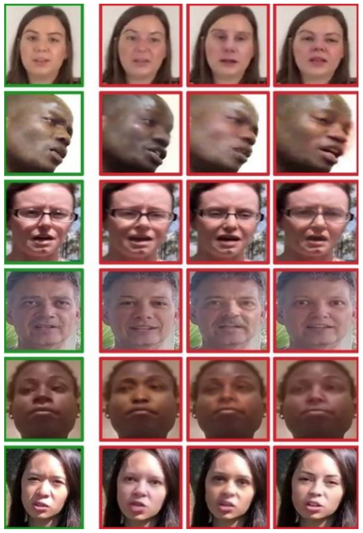Figure 2 shows samples of the detections that MTCNN wrongfully considered faces with high confidence in crowded frames.

The first stage of iCaps-Dfake is data preparation where faces are detected, for our network to train on, from the input video using YOLO v3. In order to down sample from nearly 2.2M training frames in the dataset, a sliding window scheme for keyframe selection is followed with a window width of one. As shown in Figure 3, the first frame $F_0$ is selected as a start then the window is slid by N frames to take the next. In each selected frame, the largest face is detected.

In order to detect the face, YOLO v3 performs a single forward propagation pass through which a CNN is applied once to the selected frame to deduce face scores. This is achieved by splitting the frame into a grid of size M × M such that the confidence score is calculated for B bounding boxes contained in each cell thus reflecting the certainty of having a face at each’s center. Each box is represented by five measurements (x, y, w, h and confidence) modelling the center of the face as (x, y) coordinates along with the width, height and confidence showing the probability of a box to include a face.

3.2. Feature Extraction

To extract features from the faces detected by YOLO, two different techniques were applied: CNN-based method and a texture-based analysis method. Both methods will be explained in detail in the following subsections.

3.2.1. CNN-based Feature Extraction

To enhance the feature extraction capability of the CNN, an extra preprocessing step was added. The following subsections explain the preprocessing and the feature extraction model.

Preprocessing

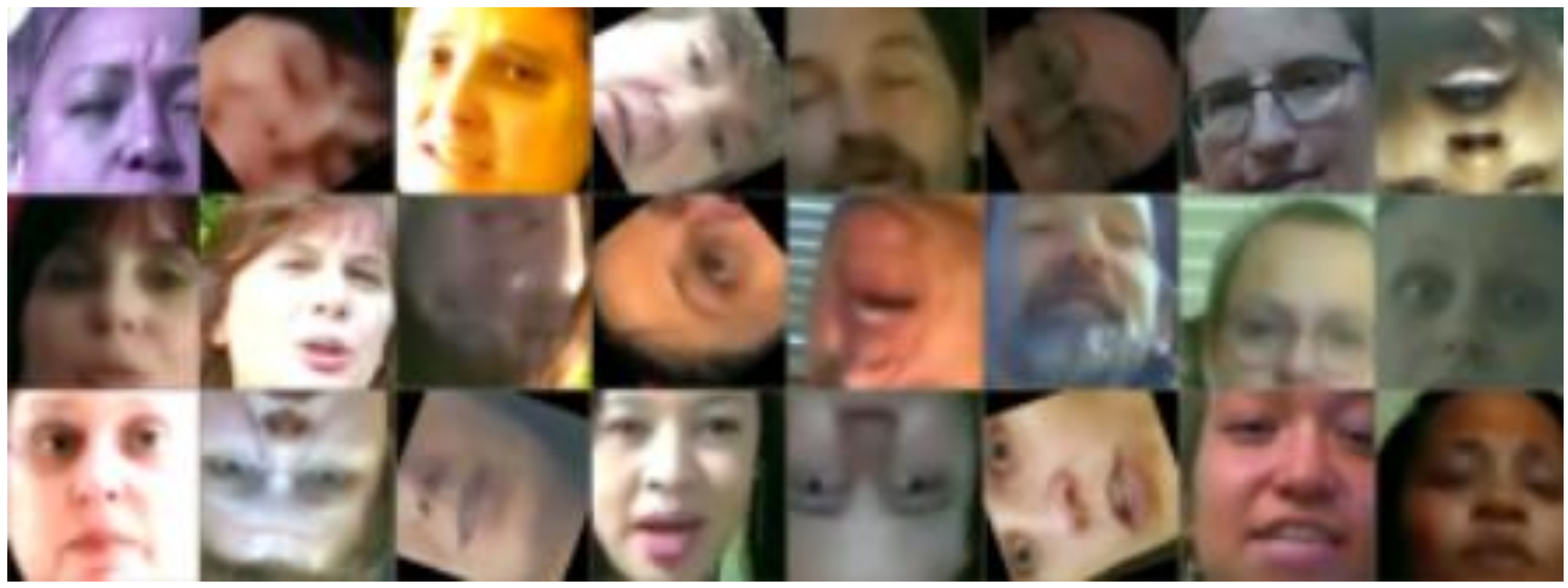
In order to train the HRNet [65], preprocessing of the extracted faces is required to provide the CNN a variety of examples thus improving the learning process. First, the detected faces are normalized and resized to 300 × 300 then randomly cropped to 224 × 224 thus enhancing the model’s capability to detect fake faces even if it exists only in a fraction of the face. Second, different random augmentations are applied such as rotation, horizontal and vertical flipping and change of the color attributes of the image. Figure 4 shows a sample of the HRNet input faces after preprocessing.

HRNet

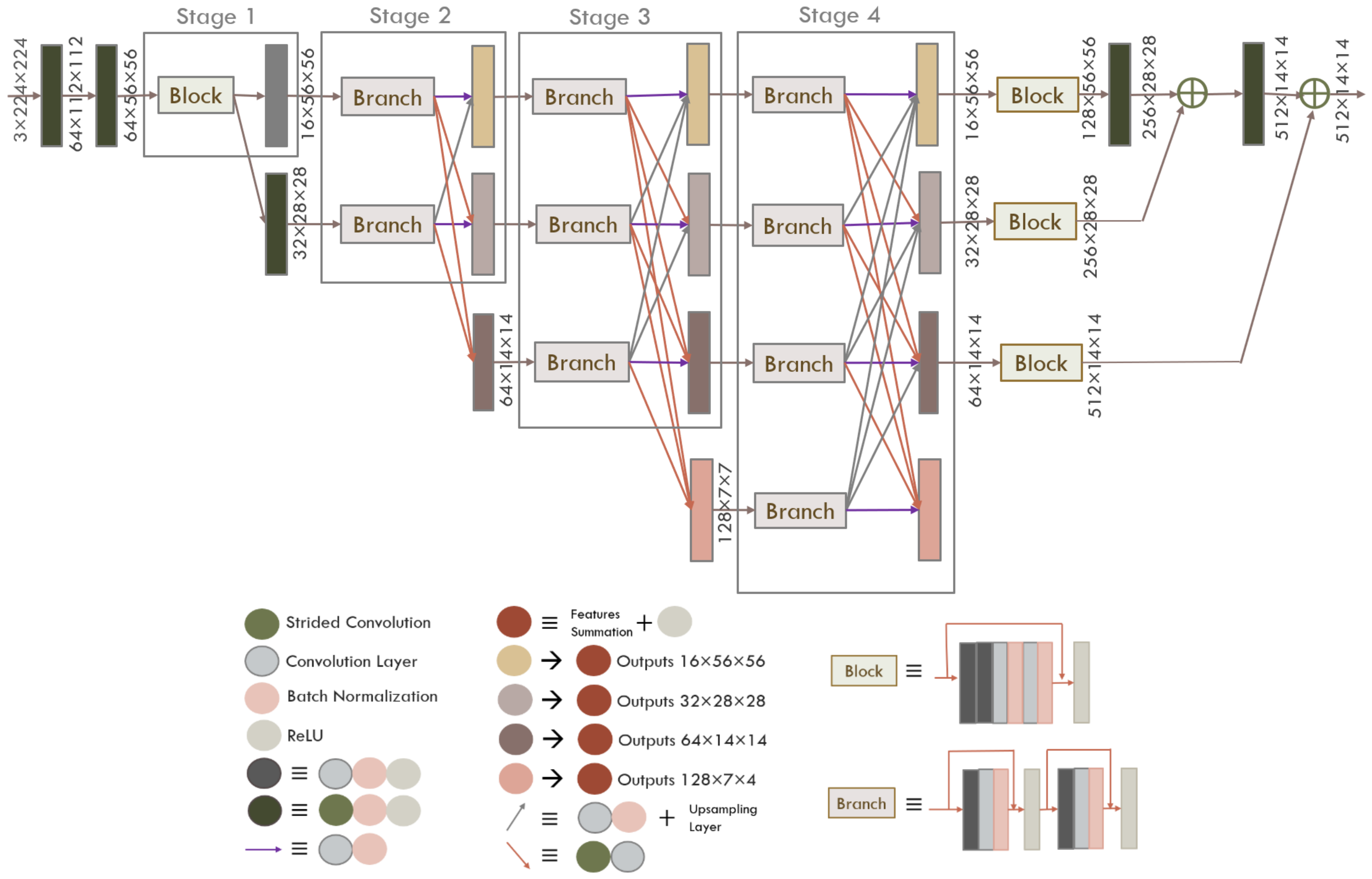
The basic concept of the HRNet was to avoid the loss of any spatial information, which seemed a good fit to that of the capsule network except that the original HRNet included a pooling layer at the end. In order to best fit the two concepts, the pooling layer from the HRNet is removed and the raw feature vector generated from the HRNet is utilized [58]. This way, the HRNet keeps the high-resolution representations across the whole process of feature extraction by connecting high-to-low resolution convolutions in parallel and producing strong high-resolution representations when repeatedly performing fusions across parallel convolutions. The output feature maps are obtained by adding the (upsampled) representations from all the parallel convolutions.

Figure 5 shows the construction of the HRNet and how the resolution changes throughout the network. It takes a 3 × 224 × 224 face and passes it through two 3 × 3 convolutions with a stride of size 2, the output of these blocks has a shape of 64 × 56 × 56. The HRNet consists of four stages where each stage is a subnetwork containing a number of parallel branches. Each branch has half the resolution and double the number of channels of the previous one, if the last branch resolution is denoted to be C then network resolutions would be 8C at the first branch, 4C, 2C and C. One branch consists of two residual blocks [66] where each contains two 3 × 3 convolutions.

The first stage is a high-resolution subnetwork that consists of one residual [66] block with four different size convolutions and outputs 16 × 56 × 56 feature vector. The following three stages contains high-to-low resolution subnetworks added gradually one by one. Stage two has two branches resembling two different resolution; The first branch preserves the resolution of the first stage and propagates it through the other stages and the second contains the down sampled resolution that is obtained by applying a 3 × 3 convolution with the stride 2 to get the feature vector of size 32 × 28 × 28 that will also propagate to the end of the stages. There is a fusion layer between each consecutive stage, it is responsible for adding different feature vectors coming from each parallel branch. To achieve this, all the feature maps need to be of the same size so different resolutions are either down sampled through strided convolution or up sampled using simple nearest neighbor sampling [67]. At Stage 4, the output of the first three branches is passed through the residual lock used at stage one in order to regulate number of channels in order to add the feature maps and obtain the output of the network of size 512 × 14 × 14.

3.2.2. Texture Analysis—LBP

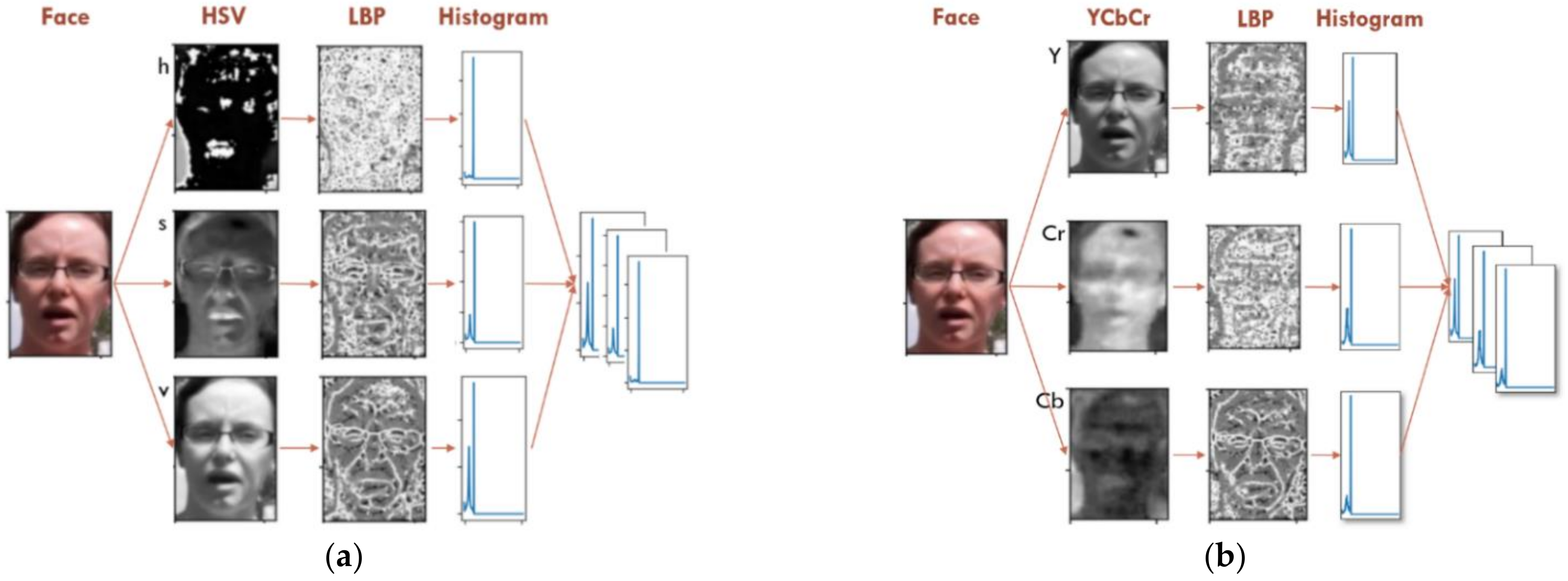
To perform texture analysis, the LBP [68] for each channel of two different color spaces (HSV and $Y{C}_b{C}_r$) is extracted and then a histogram for each LBP is calculated. The extracted histograms are then resized and concatenated to the feature maps extracted from the HRNet. Figure 6 shows the steps needed to extract histograms of the LBPs.

To perform color texture analysis, the luminance and chrominance components of the detected faces are extracted by converting them to both HSV and YC_bC_r color spaces. The RGB (red, green and blue) color space was not useful in this analysis due to its imperfect separation of the luminance and chrominance information and the high correlation between its color components.

In the HSV color space, Hue (H) and Saturation (S) represent chrominance while Value (V) corresponds to luminance. In the YC_bC_r color space, the luminance is represented in the (Y) component while both the ($C_b$) and ($C_r$) represent Chrominance blue and Chrominance red, respectively. The output shape of this step is 6 × 224 × 224 for which the LBP of each channel will be calculated.

For calculating the LBP, a local representation of texture is computed for one channel at a time by comparing each center point with its surrounding eight neighbors. The center point is used as a threshold, if the intensity of a neighbor is greater than or equal to that threshold then it is updated to the value one, otherwise zero. After this step, the eight-bit representations can be used to formulate up to 256 different decimal values which is then set to be the new value of the center point. The LBP output can be represented as a gray scale image highlighting the face texture. Figure 7 shows the output LBPs given a sample face as input for each channel along with the calculated histograms. The final step is to concatenate the six histograms, reshape them and normalize their values making a feature vector of size 4 × 14.

3.2.3. Feature Concatenation

The final step of the feature extraction phase is concatenation where the features extracted from the HRNet are combined with those of the LBP. The HRNet output is represented as a 512 × 14 × 14 feature vector are then concatenated to the 6 × 14 × 14 feature vector produced by the 6 histograms. The outcome of the feature extraction stage is a 518 × 14 × 14 feature vector that will be used as input to the capsule network to train and update the network weights accordingly.

3.3. Classification—Capsule Network

Regular CNNs are built based on scalar neuron representations that are capable of identifying probabilities of existence of particular features. To better detect a feature, CNNs require lots of different variants of the same type of data entity which in turn needs extra neurons leading to size and parameters expansion of the entire network. On top of that, pooling operations done by CNNs only propagate features that stand out and drop all other features thus losing a lot of spatial information. Unlike CNNs, CapsNets exploits all the spatial information to identify both the probability of feature existence as well as its location relative to others (pose information) making it viewpoint-invariant thus requiring less data.

First introduced by Sabour et al. [58], a capsule is a group of neurons in a shape of a vector encoding the pose information whose length represents the probability of an entity existence (activation probability). This makes deriving a part-whole relation given the embedded information in one computational unit representing the part easier. For example, a face’s components (eye, mouth, nose...etc.) would be embedded in the lower capsule levels along with their relative position. The routing algorithm then tries to connect each lower-level capsule to a single higher level one containing its specifications. In EM Routing [59], Hinton et al. represented the pose by a matrix and the activation probability was determined by the EM algorithm. The proposed model used the inverted dot-product attention routing algorithm [69] that applies a matrix-structured pose in a capsule.

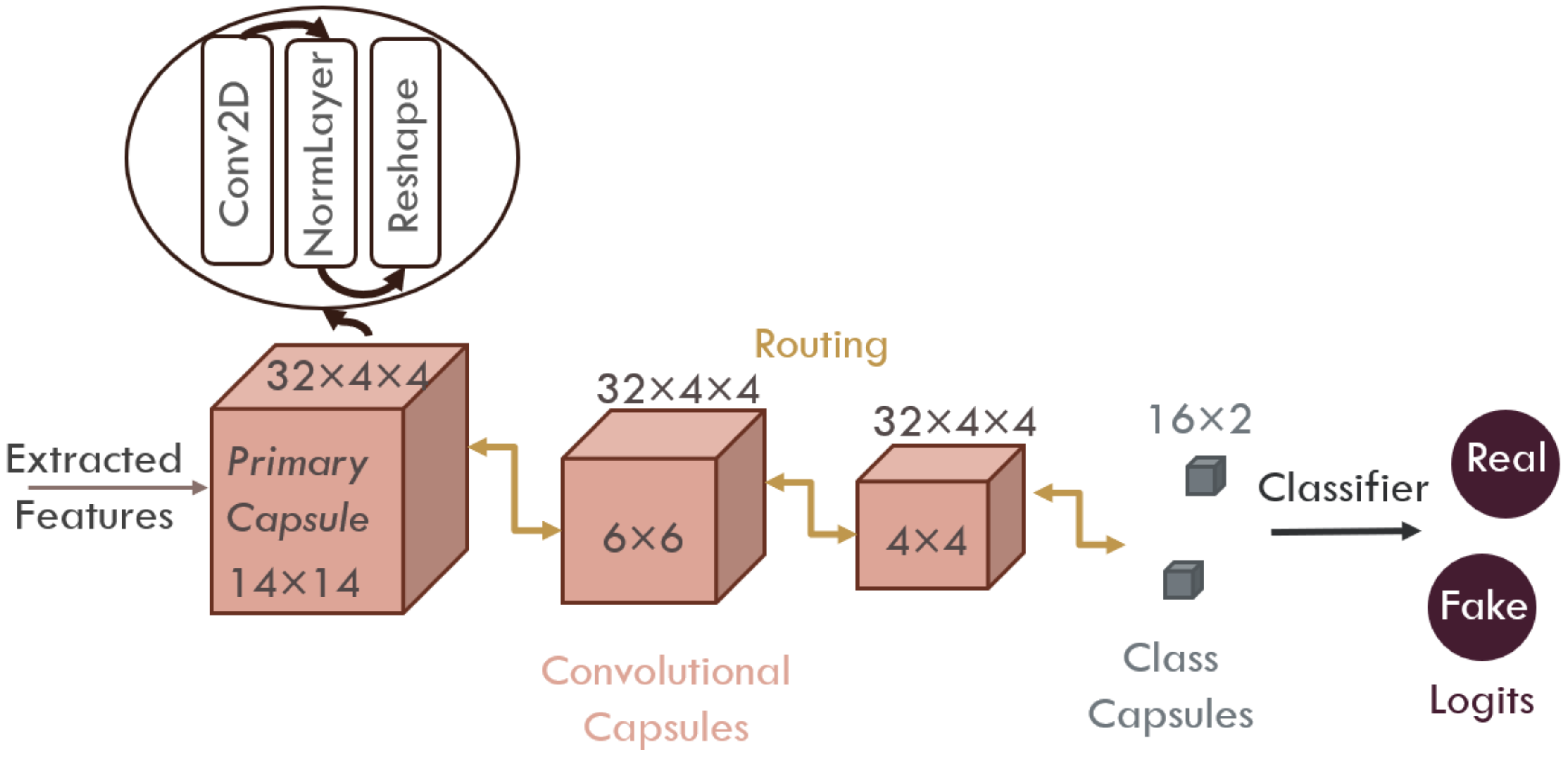
As demonstrated in Figure 8, our capsule network consists of one primary, two convolutional and two class capsules one for each class. The extracted features are fed to the primary capsule that is responsible for creating the first low-level capsules. The primary capsule applies one convolutional layer on to the extracted features then normalize the output and reshape it to create matrix-capsules of size ${ℝ}^{\sqrt{d_L} x \sqrt{d_L}}$ where $d_L$ represents the grouped number of hidden layers that define a capsule. Capsules in the primary layer (children) are used to update capsules in the first convolutional capsule layer (parents) that in turn update their parents and so forth. The convolutional capsules layers are formed using Equations (1)–(5), each containing 32 capsules of size 4 × 4.

To route a child capsule $i$ in layer $L$ ($p_i^L$) to a parent capsule $j$ in layer $L+1$ ($p_j^{L+1}$), a vote $v_{ij}^L$ is created per child for each parent by applying weights assigned between them $w_{i,j}^L$. Initially, all parents’ poses $p_j^{L+1}$ are set to zero.

$$v_{ij}^L = w_{ij}^L· p_i^L$$

(1)

By applying the dot-product similarity, the agreement $a_{ij}^L$ between each parent all children are calculated using their votes $v_{ij}^L$.

$$a_{ij}^L =p_j^{L+1^T} · v_{ij}^L$$

(2)

A routing coefficient $r_{ij}^L$ is calculated by passing the agreements scores through a softmax function.

$$r_{ij}^L = \exp \left(a_{ij}^L\right)/{{\displaystyle \sum }}_{j^{\prime }}\exp \left(a_{i{j}^{\prime }}^L\right)$$

(3)

Each child contributes in updating parents poses according to its vote $v_{ij}^L$ and routing coefficient $r_{ij}^L$.

$$p_j^{L+1} = {{\displaystyle \sum }}_i{r}_{ij}^L{v}_{ij}^L$$

(4)

Finally, a Normalization layer [70] is added to enhance the routing’s convergence.

$$p_j^{L+1} = \mathrm{LayerNorm}\left(p_j^{L+1}\right)$$

(5)

Equations (1)–(5) show the calculation steps of the capsule layers using the inverted algorithm. The first iteration is sequential, where the values of all but the first capsule layer is computed. The following iterations are concurrent thus resulting in an improved training performance.

The last capsule layers are the class capsules where the feature vector is significantly reduced to feed a linear classification layer that is used to get the prediction logits, this classifier is shared among the class capsules. Each of the two class capsules has a size of 16 and is constructed using the routing algorithm described in Equations (1)–(5).

4. Experimental Work

Our entire network was trained end-to-end so that the model backpropagates to the feature extractor for more than 20 epochs using Stochastic Gradient Descent (SGD) optimizer with momentum 0.9 and a starting learning rate of 0.001, with a decay of 1e-4. The batch size was set to 32 and the loss function is cross-entropy. The keyframe selection parameter N was chosen such that it reduced the number of training frames yet without affecting the testing evaluation. After several trials, it was set to 5 which did reduce the frame count dramatically yet had almost no effect on the test results. All our experiments were conducted on a laptop running Ubuntu 20.04 system on an Intel(R) Core(TM) i7-9750H 2.59 GHz CPU with 16GB RAM and an NVIDIA GeForce RTX 2070 with Max-Q design with 8GB memory.

4.1. Dataset

Many benchmark datasets were recently published to support the research community’s race against this drastic phenomenon. Companies like Google and Facebook have shown great interest in the deepfake detection domain as both created datasets (DFD and DFDC) to address this problem. Also, Facebook created a Kaggle competition awarding one million dollars to competitors creating the detection algorithms with the highest scores on the DFDC-P dataset [71,72].

Table 1. Datasets Summary.

Dataset	Real		Fake		Manipulation		Release Date
	Video	Frame	Video	Frame	Visual	Audio
UADFV [39]	49	17.3	49	17.3k	✓	×	2018.11
DF-TIMIT-LQ [73] DF-TIMIT-HQ	320	34.0k	320	34.0k	✓	✓	2018.12
			320	34.0k
FF-DF [34]	1000	509.9k	1000	509.9k	✓	×	2019.01
DFD [71]	363	315.4k	3068	2242.7k	✓	×	2019.09
DFDC-P [36]	1131	488.4k	4113	1783.3k	✓	✓	2019.10
Celeb-DF [35]	590	225.4k	5639	2116.8k	✓	×	2019.11

shows a summary of the most used datasets addressing this domain where the visual manipulations are precisely face replacements and only two of them included additional audio manipulations.

In [35], it was proven that Celeb-DF and DFDC-P are very challenging datasets based on calculating the average AUC metric when compared to other available datasets using Two-Stream [49], MesoNet [50], HeadPose [39], FWA [31], VA [52], Xception [34], Multi-Task [53], Capsule [61] and DSP-FWA [32] detection methods. This have led us to focus our experiments on those two reliable benchmarks on which multiple trials were performed until the best results were achieved.

DFDC-P [36] is the main dataset used to train the proposed model as it contains many extremely low-quality videos which makes it a particularly challenging dataset. It has videos for 60 different actors of which 40 were used for training and the rest for validation. The videos were created in different lightening conditions, head poses and backgrounds by actors varying in skin tone, gender and age. The distribution of gender is 74% females and 26% males having a race split of 68% Caucasian, 20% African-American, 9% east-Asian and 3% south-Asian. Different augmentations were applied on random videos such as reducing the resolution to quarter of its original, reducing the frame per second (FPS) to 15 and reducing the overall video quality. The fake videos are manipulated by two different creation methods thus improving the model’s ability to generalize on unseen methods. Figure 9 shows different samples generated from the dataset.

Celeb-DF [35] was used to verify the generalization ability of our model. This dataset was created using real YouTube videos for 62 different actors, 49 of which were used for training and the rest for validation. Also, the dataset includes additional 300 YouTube real videos of random people some of which are included in the test and the remaining in the training set. The fake manipulations are done using an improved deepfake synthesis algorithm [20] that played the main role in enhancing the visual quality as shown in Figure 10. The creation algorithm applied dealt with many artifacts that existed in previous datasets thus making it more challenging. Examples of such artifacts are low resolution of synthesized face thus outputting a face with a resolution of 256 × 256 instead of 64 × 64 or 128 × 128, color mismatch where the generated face has a monotonic color unlike before where for example the target face tone is white and the source is red, inaccurate face masks where some leftovers of the source’s face can still be seen and finally temporal flickering was reduced. The average length of all videos is approximately 13 s with the standard frame rate of 30 frames-per-second.

In

Table 2. Datasets’ distribution among the three training, validation and testing.

	Set	Train	Validate	Test	Total
DFDC-P	real	639	162	276	1131	5244
	fake	3060	549	504	4113
Celeb-DF	real	610	102	178	890	6529
	fake	4299	1000	340	5639

, the distribution of real and fake videos of both datasets used for the training, validation and testing phases are shown. For training and validation, one fifth of the video frames were used. The testing set is predefined in both datasets by the creators, all videos frames at the predefined frame per second rate are tested to be able to make a fair comparison with previously published results.

4.2. Evaluation Metrics

Eight different evaluation metrics are used to compare the performance of the proposed model with other previous attempts to detect fake videos.

4.2.1. Area Under the Curve—Receiver Operator Characteristic (AUC-ROC)

AUC-ROC [74] curve represents the level of separability in a probability-based curve. It is a commonly used performance indicator to assess the classification at different values of thresholds showing how well a model can discriminate between classes. The higher the AUC, the more separable the model is in predicting each class correctly. Two level AUC scores are reported:

• Frame-level AUC calculates the AUC for all test frame in all videos. This measure was used previously by several publications on the same chosen datasets.
• Video-level AUC calculates the AUC for all test videos. This is achieved by considering frames with classification probability more than or equal 0.5 to be fake (class 1) and others to be real (class 0) then calculating video classification score by averaging its frames probability and finally calculate the area under ROC curve score.

4.2.2. Performance Equations

We applied the following performance evaluation equations to properly assess and compare the proposed model to others. For Equations (6)–(11) [75], consider the following:

• True Negative (TN) is when the model makes a correct classification by predicting the negative class values (real) to be negative (real).
• False Positive (FP) is when the model makes a false classification by predicting the negative values (real) to be positive (fake).
• False Negative (FN) is when the model makes a false classification by predicting the positive values (fake) to be negative (real).
• True Positive (TP) is when the model makes a correct classification by predicting the positive class values (fake) to be positive (fake).

$$Accuracy= \frac{TP+TN}{TN+FN+FP+TP}$$

(6)

$$\mathrm{Precision}= \frac{TP}{TP+FP}$$

(7)

$$\mathrm{Recall}= \frac{TP}{TP+FN}$$

(8)

$$\mathrm{FPR}= \frac{FP}{TN+FP}$$

(9)

$$\mathrm{F}-\mathrm{Measure} = \frac{2 x Precision x Recall}{Precision+Recall}$$

(10)

$$\mathrm{FNR}= \frac{FN}{TP+FN}$$

(11)

4.3. Results

All video key frames from both datasets [35,36] were tested on the trained model.

Table 3. Frame-level Area-Under Curve (AUC) scores (%) for the proposed iCaps-Dfake model compared to previous detection methods when tested by DFDC-P.

Method	DFDC-P
Two-stream [49]	61.4
Meso4 [50]	75.3
MesoInception	73.2
HeadPose [39]	55.9
FWA [31]	72.7
VA-MLP [52]	61.9
VA-LogReg	66.2
Xception-raw [34]	49.9
Xception-c23	72.2
Xception-c40	69.7
Multi-task [53]	53.6
Capsule [61]	53.3
DSP-FWA [32]	75.5
iCaps-Dfake	76.8

shows frame-level AUC scores for our DFDC-P results compared to recent detection approaches. The iCaps-Dfake proposed model outperformed other models by an average 12.12% increase in the frame-level AUC.

Table 4. Frame-level AUC scores (%) for the proposed iCaps-Dfake model compared to previous detection methods when tested by Celeb-DF.

Method	Celeb-DF
Two-stream [49]	53.8
Meso4 [50]	54.8
MesoInception	53.6
HeadPose [39]	54.6
FWA [31]	56.9
VA-MLP [52]	55.0
VA-LogReg	55.1
Xception-raw [34]	48.2
Xception-c23	65.3
Xception-c40	65.5
Multi-task [53]	54.3
Capsule [61]	57.5
DSP-FWA [32]	64.6
Nirkin et al. [33]	66.0
FakeSpotter [54]	66.8
Two-Branch [38]	73.41
iCaps-Dfake (fine-tuned)	77.1
iCaps-Dfake (trained)	86.0

shows two test results for our proposed model on Celeb-DF. In the first test, an average 18.01% increase is achieved over previous methods by only fine tuning the model, that was pretrained on DFDC-P, for one epoch on Celeb-DF faces thus showing a generalization capability of the proposed model. The second experiment was performed to test the model’s results after being trained for more than 50 epochs using the Celeb-DF dataset and produced an average 26.91% increase over others.

Table 5. Video-level AUC scores (%) on DFDC-P dataset.

Method	DFDC-P
Emotions don’t lie [44]	84.4
iCaps-Dfake	87.8

and

Table 6. Video-level AUC scores (%) on Celeb-DF dataset.

Method	Celeb-DF
Two-Branch [38]	76.65
iCaps-Dfake (fine-tuned)	91.0
iCaps-Dfake (trained)	96.9

show the video-level AUC comparison between our iCaps-Dfake model and previous methods. An increase of 3.4% over the previous method on DFDC-P and 20.25% increase on Celeb-DF are reported. Figure 11 sketches the corresponding Receiver Operator Characteristic (ROC) curve for the provided results. It shows that Celeb-DF results are better than DFDC-P results although the detection rate of the former is less than the latter as previously discussed.

Table 7. Video-level Accuracy (%) on Celeb-DF dataset.

Method	Celeb-DF
Gaze Tracking [48]	88.35
iCaps-Dfake (fine-tuned)	81.85
iCaps-Dfake (trained)	91.70

shows that our trained model outperformed the video-level accuracy of a very recently published model with a 3.35% increase when compared on Celeb-DF [35]. As shown in

Table 8. Number of parameters comparison.

Method	DFDC-P Frame-Level AUC (%)	Number of Parameters
Xception [34]	49.9	20,811,050
Capsule [61]	53.3	3,896,638
iCaps-Dfake	76.8	11,715,121

, the proposed iCaps-Dfake model used an average number of parameters when compared to other methods yet there was over 20% improvement in the AUC. This shows that the increase in the number of parameters over the model presented in [61] was compensated by the huge result improvement in the AUC. Finally,

Table 9. Video-level results (%) calculated from the provided performance equations.

	Accuracy	Precision	Recall TPR	F-Measure	FPR	FNR
DFDC-P	79.41	90.12	76.45	82.72	15.22	23.55
Celeb-DF	91.70	93.29	94.12	93.70	12.92	5.88

shows our performance measures for future comparisons of the proposed model when trained and tested on the two datasets. The high value of f-measure shows that the proposed model is not biased to any of the two classes thus it can easily discriminate between real and fake videos/images.

5. Discussion

In this research, a new deepfake detection model (iCaps-Dfake) is proposed that combined texture feature extraction with HRNet based method to train a capsule network to improve the classification accuracy. The proposed model results show great improvement over other state-of-the-art methods. The selection of YOLO-v3 as a face detector led to great reduction in false positive faces predictions thus reducing the need for further preprocessing steps. The fusion between two different in nature feature extraction approaches enriched the model and helped it learn better. The texture-based approach using the LBP provided an artifacts-specific flavor to our model by counting on the difference between textures of the fake face and the surrounding background. The CNN-based using HRNet provided our capsule network with informative-representations while preserving the capsule concept of not losing any spatial information to get the most out of small details. The augmentation-normalization step performed on images that were input to the HRNet helped in enhancing the results. The CapsNet with its advantageous performance in feature abstraction and classification tasks made a robust decision whether the introduced image is fake or real. Our results were compared to other sophisticated models and showed not only an improvement in the AUC but also a generalization capability of the proposed model. For DFDC-P, it achieved an average 12.12% improvement in the frame-level score and 3.4% at the video-level score. For Celeb-DF, the proposed model attained an average 18.01% increase in frame-level score and 14.35% increase in video-level score. It also scored an average 26.91% increase in frame-level and 20.25% increase in video-level when further training the model on Celeb-DF. In the future, a plan is made to expand the model such that it can also handle fake audio embeddings and try to achieve even higher results.