Abstract
In real applications, massive data with graph structures are often incomplete due to various restrictions. Therefore, graph data imputation algorithms have been widely used in the fields of social networks, sensor networks, and MRI to solve the graph data completion problem. To keep the data relevant, a data structure is represented by a graph-tensor, in which each matrix is the vertex value of a weighted graph. The convolutional imputation algorithm has been proposed to solve the low-rank graph-tensor completion problem that some data matrices are entirely unobserved. However, this data imputation algorithm has limited application scope because it is compute-intensive and low-performance on CPU. In this paper, we propose a scheme to perform the convolutional imputation algorithm with higher time performance on GPUs (Graphics Processing Units) by exploiting multi-core GPUs of CUDA architecture. We propose optimization strategies to achieve coalesced memory access for graph Fourier transform (GFT) computation and improve the utilization of GPU SM resources for singular value decomposition (SVD) computation. Furthermore, we design a scheme to extend the GPU-optimized implementation to multiple GPUs for large-scale computing. Experimental results show that the GPU implementation is both fast and accurate. On synthetic data of varying sizes, the GPU-optimized implementation running on a single Quadro RTX6000 GPU achieves up to speedups over the GPU-baseline implementation. The multi-GPU implementation achieves up to speedups on two GPUs versus the GPU-optimized implementation on a single GPU. On the ego-Facebook dataset, the GPU-optimized implementation achieves up to speedups over the GPU-baseline implementation. Meanwhile, the GPU implementation and the CPU implementation achieve similar, low recovery errors.
1. Introduction
With the rapid development of social networks, e-commerce, and the Internet, a large amount of graph-structure data has been generated. User profiles in social networks, user-item matrices in recommendation systems, and sensory data in the Internet of Things can be modeled as feature matrices [1]. These matrices with the graph structure can be represented as the graph-tensor by stacking them in vertex order [2]. However, due to limitations in the data collection and measurement process [1], it is ubiquitous that only a subset of data matrices is observed while some data matrices are fully unobservable. These incomplete data introduces difficulties for later data mining and analysis. Therefore, various tensor completion methods have been designed to recover the incomplete data in different situations.
Exiting works studied the data completion problem of tensors with missing elements [3], tubals [4], or matrices [2,5]. Figure 1 shows an example of missing data matrices. In this social network (i.e., a graph), each user has a data matrix, but the data matrices for users and are entirely unobservable. We obtain an observed graph-tensor by stacking data matrices in vertex order and taking vertex order as the third dimension of the graph-tensor. To complete the observed graph-tensor, Sun et al. proposed a convolutional imputation algorithm to recover the graph-tensor [2]. However, with the growing data size or dimension of tensors, the execution time of the CPU-based convolutional imputation algorithm increases rapidly [5], making it impractical for efficient big-data processing or applications with real-time requirements.
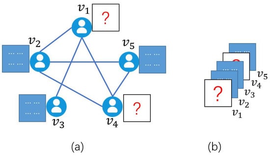
Figure 1.
(a) A social network represented as a graph. (b) A graph-tensor corresponds to the graph of (a).
In this paper, we propose a high-performance, Graphics Processing Unit (GPU)-based graph-tensor imputation scheme for large-scale graph data and social network applications. We design, implement, and optimize an efficient convolutional imputation algorithm on single and multiple GPUs by exploiting multi-core GPUs of CUDA architecture. First, we design and implement a baseline graph-tensor imputation algorithm on GPU. Second, we investigate the performance bottlenecks of the baseline implementation and explore stream computing and batched computing techniques to optimize the utilization of GPU SM resources and CPU-GPU communications for higher performance. Third, in order to support large-scale graph-tensor imputation, we propose a multi-GPU computing scheme to utilize more memory and computing resources of multiple GPUs on a computing node.
Our contributions are summarized as follows.
- We design and implement the convolutional imputation algorithm on GPU to achieve high performance and accuracy. The GPU-based convolutional imputation algorithm includes an efficient graph Fourier transform operation with coalesced memory accesses to achieve high parallelism.
- We propose effective optimization strategies to improve GPU utilization, including stream computing and batched computing. To support large-scale graph-tensor imputation and further improve performance, we propose a multi-GPU computing scheme to perform the computation on multiple GPUs.
- We perform extensive experiments to evaluate the performance of the GPU-based convolutional imputation algorithm using both synthetic and real data. With synthetic data, the GPU-optimized implementation achieves up to speedups versus the GPU-baseline implementation running on a Quadro RTX6000 GPU. The multi-GPU implementation achieves up to speedups on two GPUs versus the GPU-optimized implementation on a single GPU. The GPU implementation achieves similar recovery errors with the CPU MATLAB implementation. For the ego-Facebook dataset with various sampling rates, the GPU-optimized implementation achieves up to speedups versus the GPU-baseline implementation running on a Quadro RTX6000 GPU, while achieving similar recovery errors.
The remainder of this paper is organized as follows—Section 2 reviews the related works. In Section 3, we describe the notations and the convolutional imputation algorithm. Section 4 presents the design, implementation, and optimization of the graph-tensor imputation algorithm on GPU. We scale the optimized GPU implementation onto multiple GPUs in Section 5. In Section 6, we evaluate the performance of the GPU-based graph-tensor imputation algorithm. The conclusions are drawn in Section 7.
2. Related Works
We discuss the related works on graph applications, tensor completion, GPU-based tensor computing and research on high-performance GPUs.
Graph, as an important data structure, has strong expressive ability, and has wide applications in many fields. In the field of data mining, a variety of graph processing systems have been developed, from GraphChi [6], which is a CPU-based system for computing large-scale graphs on a single machine, to the multi-GPU based system Gunrock [7], to Gluon [8] which is a distributed heterogeneous (CPU+GPU) graph analytics system. These systems provide a high-level API for implementing graph analysis algorithms, such as PageRank (PR), connected components (CC), and single-source shortest path (SSSP). GSPBOX [9] and PyGSP [10] are two CPU-based graph signal processing libraries that provide a variety of graph operations, including graph Fourier transform. In the field of deep learning, the concept of graph neural network (GNN) was first proposed in [11], which extends the existing neural network for processing data in the graph domain. In recent years, a set of neural network theory based on graph convolution operation has been developed and continuously derived [12,13].
Low-rank tensor completion is an important research filed for the data reconstruction problem. It can be applied to recommender systems [14], MRI data recovery [15], video decoding or inpainting [16], and so on. However, these studies only focus on the low-rank approximation to estimate missing values; thus, they cannot sufficiently exploit the relevance of information structure. Recently, Sun et al. [2] proposed the convolutional imputation algorithm to recover graph-tensor by utilizing the graph structure for the scenario where the data of some vertices are completely missing. The algorithm utilizes GFT to transform the graph-tensor from the spatial domain to the spectral domain, which could expose more parallelisms and brings an opportunity for high-performance computing.
Some existing works [3,4,17] proposed high-performance algorithms for tensor completion. Their algorithms converted a tensor completion problem into a set of parallel matrix completions in the frequency domain, then use a matrix completion algorithm to complete each slice matrix, and finally convert the results back to the time domain. Liu et al. proposed a fast iterative tensor completion algorithm called Tubal-Alt-Min based on the low-rank matrix completion [3]. As the Tubal-Alt-Min algorithm has high parallelism, Zhang et al. implemented this algorithm on GPU in the cuTensor-tubal library [17] for high performance. Inspired by these researches, we implement the convolutional imputation algorithm [2] on high-performance GPUs to improve efficiency in applications. However, in order to utilize the GPU effectively, some challenges must be addressed, including data transfer, memory access, and appropriate parallelization schemes for graph-tensor computations.
High-performance GPUs have been increasingly adopted in data processing to improve efficiency. Abdelfattah et al. [18] designed effective thread and kernel scheduling strategies to accelerate dense matrix-vector computations. Jia et al. [19] exploited multiple GPUs to accelerate the execution of Lux system by combining coalesced memory access with shared memory access. Zhang et al. [20] design a multi-GPU scheme for homomorphic matrix completion to make full use of multiple GPUs on a single node and accommodate large-scale data. The convolutional imputation algorithm [2] is based on the iterative calculation of singular value soft-threshold, which includes compute-intensive SVD computation. We compare and utilize the SVD routines in cuSLOVER and KBLAS GPU libraries. We further propose optimization strategies on kernel design, memory accesses, and batched computing to improve algorithm performance.
3. Convolutional Imputation Algorithm
We introduce the notations, summarize the convolutional imputation algorithm [2], and provide parallel acceleration analysis for this algorithm.
3.1. Notations
We use lowercase boldface letters to denote vectors and uppercase boldface letters to denote matrices. Let index the rows and columns of a matrix, respectively, and or to denote the -th matrix entry. Third-order tensors are denoted by uppercase calligraphic letters, . Let index the first, second, and third dimensions of a tensor, respectively, and or to denote the -th entry. Let denote the set , then , , unless otherwise specified. Please refer to Table 1 for the notations of major symbols.

Table 1.
Major symbols.
Graph-Tensor: a weighted graph is defined by , where is a set of N vertices and E is a set of edges. We use the weighted adjacency matrix to describe the the relationship between vertices in the graph. Two vertices and are adjacent if is an edge, . Let denote the weight on the edge , otherwise, let .
Assuming the data on each vertex is a matrix of size , we define a graph-tensor by stacking data matrices of all vertices along the third dimension. The data matrix of the k-th vertex is denoted by or for simplicity. The Frobenius norm of a graph-tensor is .
Tubes and slices: a tube (also called a fiber) is a 1D vector defined by fixing all indices but one, while a slice is a 2D matrix defined by fixing all but two indices. Tubes can be categorized into model-1, model-2, and model-3 tubes, and slices can be categorized into frontal, lateral, and horizontal slices [3]. We use to denote the -th model-3 tube and to denote the k-th frontal slice. We call or the data matrix if it is a vertex value, and frontal slice otherwise.
Graph Fourier Transform (GFT): the graph Fourier transform extends the concept of the discrete Fourier transform to a general graph, which is to transform a graph signal in the spatial domain into the spectral domain. For a graph with the adjacent matrix , the normalized graph Laplacian matrix is defined as , where is a diagonal matrix with entries . The graph Fourier transform matrix , a unitary matrix, is given by the eigendecomposition of , where columns of are the eigenvectors of , and is the diagonal matrix whose diagonal elements are eigenvalues of .
The graph Fourier transform (GFT) of a graph-tensor is defined as , where is a stack of N matrices in the spectral domain of the graph. Furthermore, each frontal slice in the spatial domain is a linear combination of data matrices on the graph, . The inverse graph Fourier transform (iGFT) is defined as , correspondingly.
Convolution of Graph-Tensors: in the Convolution Theorem, the convolution in the time domain corresponds to point-wise multiplication in the frequency domain. We generalize it to graph-tensors, which is defined as multiplication in the spectral space. Given two graph-tensors on the same graph, we define their convolution as . Then, we denote a stack of matrices as , where each matrix is the matrix multiplication of and .
For more detailed definitions of the graph-tensor and related operations, please refer to [3,21,22,23].
3.2. Overview of the Convolutional Imputation Algorithm
The convolution imputation algorithm [2] was proposed for recovering missing slices in a graph tensor (i.e., here we consider the case of missing slices, the slice-sampling pattern). In the slice-sampling pattern, the data matrix of each vertex is either fully observed or fully missing. Figure 1 shows an example of a social network that can be abstracted into a graph . Each user is represented by a vertex , and each relationship between users is represented by an edge . The graph-tensor in Figure 1b is composed of the data matrix of each vertex, in which two frontal slices are missing due to the complete loss of users and ’s information. To recover the missing slices is a graph-tensor completion problem in the slice-sampling pattern.
The pseudo code of the convolutional imputation algorithm [2] is given in Algorithm 1. We use to denote the slice-sampling index set, and is a complement set to . The projection operator is defined to sample the graph-tensor by retaining only entities that are indexed in the set . Given an observed low-rank graph-tensor , a graph Fourier transform matrix , and a sequence of regularization parameters , the imputation algorithm [2] iteratively performs imputation of and singular value soft-threshold of to find the minimizer of the optimization problem. According to the convolution of graph-tensors, in the spectral domain, we denote singular value soft-threshold as , where means keeping only positive values, and is the singular value decomposition (SVD), , .
| Algorithm 1: Iterative convolutional imputation. |
Input: , number of iterations C, maximum number of iterations T.
|
For in each iteration, the algorithm selects the maximum singular value of as , and decays at a constant speed . For more details on convergence and computational complexity, please refer to [2].
3.3. Parallel Acceleration Analysis
We use Figure 2 to analyze the parallelism of the convolutional imputation algorithm [2]. The algorithm consists of three nested loops, the first loop (the outermost for-loop) executes C times, and the second loop (the while-loop) will break out if it reaches the maximum number of iterations T or the convergence criteria. However, these two loops cannot be executed in parallel because both of them depend on the previous result of . On the other hand, in the third loop, we can compute the singular value soft-threshold for N matrices in parallel.
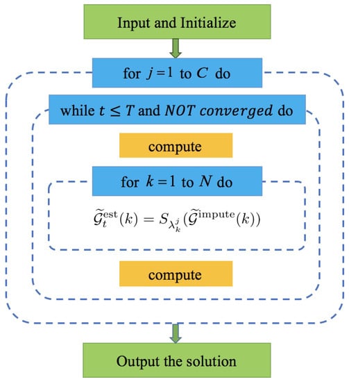
Figure 2.
The overall flow chart of the convolutional imputation algorithm.
In the CPU MATLAB implementation of the convolutional imputation algorithm, the computing time of graph Fourier transform and inverse graph Fourier transform accounts for more than 50% of the total running time, and the computing time of singular value soft-threshold accounts for more than 45% of the total running time. These operations of the graph-tensor corresponding to lines 8–10 in Algorithm 1 involve matrix multiplication and matrix singular value decomposition, which can exploit parallel computing on GPU for acceleration. Specifically, there are graph Fourier transform on mode-3 tubes of that can be computed in parallel on GPU. Similarly, there are inverse graph Fourier transform that can be parallelized on GPU. Besides, exploiting the convolution theorem of graph-tensors, the computing of N singular value soft-threshold on frontal slices of can be conducted in parallel on GPU in the graph spectral domain. Therefore, we focus on the design, implementation, and optimization of lines 8–10 in Algorithm 1 on GPU to obtain a high-performance convolutional imputation algorithm.
4. Efficient Convolutional Imputation Algorithm on GPU
We parallelize the convolutional imputation algorithm in Algorithm 1 on GPU by designing data storage and mapping algorithm steps onto the GPU architecture. Inspired by the optimization of memory access in [17,19], we take the idea of coalesced memory access to optimize GFT in the baseline GPU implementation. Then we mainly focus on the compute-intensive operation SVD and propose techniques to improve the utilization of GPU resources, memory bandwidth utilization, and overlap CPU-GPU communication.
4.1. Design and Implementation of the Baseline GPU Convolutional Imputation Algorithm
4.1.1. Computing in the Graph Spectral Domain
For the convolutional imputation of graph-tensors, we convert it into the graph spectral domain for computing, which generally includes the following three steps:
- First, transform the incomplete graph-tensor into the graph spectral domain by applying graph Fourier transform along the third dimension.
- Then, perform the matrix imputation task for each frontal slice of the graph-tensor.
- Finally, transform the completed graph-tensor back to the time domain by applying the inverse graph Fourier transform along the third dimension.
4.1.2. Data Storage
The above three steps access the tubes and slices of the graph-tensor alternately. The first and the third steps fetch and store tubes while the second step fetches and stores slices. Since the structure of memory hardware is a 1D linear space, we use a 1D arrays for data storage. In addition, because CUDA libraries [24] access the matrix in the column-major format, we store each frontal slice of the graph-tensor in the column-major format. For a graph-tensor with each frontal slice representing a vertex value, we unfold it in slice-by-slice, column-major layout as a 1D array in CPU and GPU memory. of size is squeezed into an array of size . As shown in Figure 3, we store the graph-tensor as a 1D array in memory, where different frontal slices are represented by different colors.
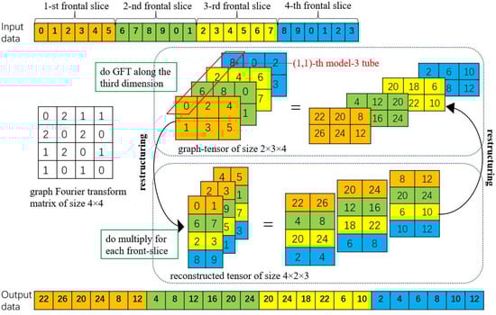
Figure 3.
Reconstruction of graph-tensor data for computing graph Fourier transforms in the batched scheme.
4.1.3. Parallelization of the Algorithm
In Algorithm 1, the major computations are graph Fourier transform, inverse graph Fourier transform, and singular value soft-threshold in lines 8–10 in each iteration. Since the process of inverse graph Fourier transform is quite similar to the process of graph Fourier transform, we only discuss graph Fourier transform in the following sections for conciseness. For the outermost for-loop, we set the configurable parameter C as the number of iterations, and is the regularization parameter for iteration j. The result for iteration j with is a start for the next iteration with . For the nested while-loop, the program ends in the maximum iterations T or the convergence condition satisfies the formula , where is an adjustable parameter that can affect the result of computing and . In the while-loop:
- For the graph Fourier transforms computation in line 8 of Algorithm 1, the algorithm accesses data along the third dimension of the graph-tensor. That is to access the graph-tensor model-3 tube by model-3 tube. Based on the data storage mentioned earlier, it cannot provide coalesced memory access for the GFT computation on GPU. The premise of coalesced memory accesses is that accesses must be sequential and addresses aligned. Therefore, we introduce the step of data reorganization. First, we utilize the eigenvalue solver method provided in the cuSLOVER library [24] to get the graph Fourier transform matrix , which is composed of eigenvectors of the graph Laplacian matrix . Then, we propose a mapping to reconstruct the graph-tensor , where the original slice-by-slice layout (the index of is ) of data is reorganized into the tube-by-tube layout (the index of is ). Finally, we utilize batched matrix-matrix multiplication in the cuBLAS library [24] to calculate the GFT of , and then convert the result back to the original data layout in the graph spectral domain to get . Since the benefits obtained from batched matrix multiplication far outweigh the overhead introduced by reorganizing the data, the overall algorithm performance is improved.We design a batched scheme for the GFT computation by reorganizing the graph-tensor data to improve parallelism. Figure 3 shows an example to illustrate the detailed scheme. For a graph-tensor with size and graph Fourier transform matrix with size , the original computation is that each frontal slice in the graph spectral domain is a linear combination of data matrices on the graph, where data access is random. The result of is the dot product of vector and , 0 🞷 0 + 2 🞷 6 + 1 🞷 2 + 1 🞷 8 = 22. However, it is more time consuming because random accesses to the data are slower than sequential accesses. Therefore, we reorganize the graph-tensor data to achieve sequential accesses, such as the -th model-3 tube is reorganized into the 1st-column of 1-st frontal slice, the -th model-3 tube is reorganized into the 2nd-column of 1-st frontal slice, and so on. The graph Fourier transform matrix can now multiply each frontal slice matrix in batched by exploiting batched matrix-matrix multiplication.
- For the singular value soft-threshold computation in line 9 of Algorithm 1, it includes singular value decomposition and matrix multiplication for each frontal slice, as shown in the the pseudo code in Algorithm 2. To perform SVD of each frontal slice of , we utilize the cusolverDnSgesvdj(.) routine in the cuBLAS library [24], which is implemented via the Jacobi method and is faster than the standard method. Besides, we arrange the computations in Algorithm 2 into batched computation to achieve better parallelism and performance. Because only stores non-zero diagonal elements, we design a GPU kernel to batch the execution of N matrices (line 3), where each thread is responsible for an element of tensor (i.e., is paired with thread ). Considering that tensor of size , tensor of size and tensor of size in SVD results are stored in 1D arrays of size , and , respectively, the value of with the index in the 1D array is . Using this kernel is more efficient than calling the cuBLAS library API for each frontal slice. Further, we convert the diagonal matrix to the left of the operator (Figure 4a) rather than the right (Figure 4b) to allow for the coalesced memory access to the device memory. As shown in Figure 4a, threads access contiguous memory blocks, and so they are benefiting from coalesced memory access instructions for better efficiency. In line 4, we utilize a routine in the cuBLAS library to perform the batched matrix-matrix multiplication on N matrices in parallel.
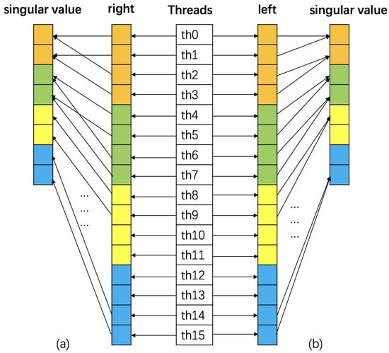 Figure 4. Thread mapping to perform the diagonal matrix-matrix multiplication of a batch of matrices. The diagonal matrix in (a) is to the left of the operator, which enables coalesced memory access to device memory, and in (b) is to the right of the operator.
| Algorithm 2: Implementation of singular value soft-threshold. |
Input: graph-tensor in the graph spectral domain, regularization parameter of iteration j, number of vertex N.
|
4.2. Optimizations
We performed some preliminary experiments to evaluate the baseline GPU graph-tensor convolutional imputation algorithm on a small dataset and found that it achieved less than 10× speedup versus the CPU MATLAB implementation. Therefore, we diagnose and optimize performance bottlenecks.
4.2.1. Performance Bottlenecks Analysis
We analyzed the baseline GPU implementation using the CUDA profiler [24] and observed three major bottlenecks: low memory copy overlap, low utilization of GPU compute units and long execution time of SVD. We consider optimizing the baseline GPU implementation on these aspects.
4.2.2. Optimizing SVD Computation
On GPUs, CUDA streams can be used to overlap computations and communications because the hardware compute engine and copy engine are independent of each other. We utilize two streams for data transmission and computation, respectively, to overlap their execution and improve efficiency.
The execution time of SVD computation (line 2 of Algorithm 2) accounts for a large proportion of the total time. In the baseline GPU implementation, for with a stack of N frontal slices of size , we use the matrix SVD routine cuSOLVER library to compute SVD of these N frontal slices sequentially on GPU. This leads to low performance, primarily for two reasons. First, a matrix SVD on a single frontal slice is inadequate to utilize all thousands of computing cores on GPU, especially for graph-tensors with a small size of frontal slices. Second, kernel launch overhead is incurred every time the matrix SVD routine is called. This kernel launch overhead is especially high for graph-tensors with a large N. In order to improve GPU utilization and the performance of SVD computation, we consider to pack these N matrix SVDs into a batch to compute them parallel using a single GPU kernel. Note that N can be large if GPU has enough device memory. This is suitable for the social network application in the experiment section, where the data matrix of vertex is small, but the number of vertices is greater than thousands.
The cuSOLVER library provides a batched method to calculate multiple SVD in parallel. However, the size of the matrix is limited to or smaller. Therefore, we utilize the KBLAS library [18], which provides batched SVD routines for matrices with a maximum size of . Therefore are multiple batched SVD routines in the KBLAS library, but none of them returns a matrix composed of right-singular vectors. Let the singular value decomposition of a graph-tensor in spectral space be with size , the KBLAS library only provides of size containing left-singular vectors, of size containing singular values, and of size . Here we set the rank of to n. Therefore, besides utilizing the batched SVD routine in the KBLAS library, we design a kernel to obtain the right-singular vectors in the batched method by computing in parallel. In this kernel, each GPU thread corresponds to one element of the tensor , as shown in Figure 4b.
5. Large-Scale and Multi-GPU Graph-Tensor Imputation
Real-world graphs such as Facebook and Twitter networks have more than one billion vertices, which poses challenges for the graph-tensor imputation on a single GPU because of limited computing cores and device memory. The SVD computation consumes lots of device memory, including the buffer size calculated by cusolverDnDsyevd_bufferSize(.) and variables that store the calculated results. In addition, the required computing cores increase rapidly with the growing size of graphs. Therefore, it is beneficial to scale the GPU convolutional imputation algorithm onto multiple GPUs in order to support the computing of large-scale graph-tensors that beyond the device memory capacity of a single GPU. We design a multi-GPU scheme for the convolutional imputation algorithm, as shown in Figure 5. Since the data reorganizing step in GFT and iGFT computation requires the entire graph-tensor as input, and the computing time of GFT and iGFT only accounts for a small part of the total time, the multi-GPU scheme is focused on the computation of singular value soft-threshold on multiple GPUs, which includes the compute-intensive SVD operation.
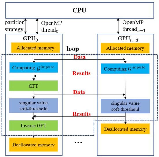
Figure 5.
Multi-Graphics Processing Unit (GPU) scheme for the convolutional imputation algorithm.
The multi-GPU scheme uses CUDA and OpenMP as a hybrid. Assuming that there are n GPUs on a computing node, the scheme use n OpenMP threads to control n GPUs for computation and communication, respectively. In the scheme, after allocating memory for input and on all GPUs, the scheme performs the following major steps in each algorithm iteration:
- GPU utilizes a partitioning strategy to split the frontal slice of into n partitions, then sends a partition to each of the other GPUs by using a peer to peer, asynchronous memory transferring routine in the CUDA library [24]. Each GPU computes its own part of independently and sends the result back to GPU;
- GPU performs synchronization to ensure results are received from all GPUs, then performs GFT computation to obtain ;
- GPU utilizes a partitioning strategy to split into n partitions, then sends a partition to each of the other GPUs by using a peer to peer, asynchronous memory transferring routine. All GPUs perform singular value soft-threshold computation with their own data independently. After the completion of computation, each of the other GPUs sends the result back to GPU.
- GPU performs synchronization to ensure all GPUs finish their tasks and then performs the iGFT computation.
In this scheme, using OpenMP threads achieves overlap of communications and eliminates the use of cudaSetDevice(.) routine in the CUDA library to switch GPU during computation. Besides, we utilize peer to peer, asynchronous communications between GPUs, which transfers data between a pair of GPUs directly without accessing CPU memory. To make full use of device memory, variables are immediately released when they are no longer needed in each step.
The data partition strategy is based on GPU hardware performance that can be obtained from the GPU specification on the NVIDIA website [25,26]. The size of the data partition received by a GPU is proportional to its hardware performance. For instance, we use to denote the performance of GPU, then GPU receives frontal slices for processing, where is the number of frontal slices distributed to GPU and , .
6. Performance Evaluation
We describe the detailed experiments settings of the GPU- and CPU-based convolutional imputation algorithms. We evaluate algorithm performance in terms of running time and recovery errors.
6.1. Evaluation Settings
6.1.1. Experiment Datasets and Configurations
We use both synthetic graphs and real social networks in experiments. The synthetic graphs are generated according to [2], where the adjacency matrix of a sparse graph is randomly generated, and the graph-tensor is generated by performing iGFT operation on a stack of low-rank matrices in the graph spectral domain. A low-rank matrix of rank r in size is obtained by multiplying two i.i.d Gaussian random matrices in size . Then we obtain the observed graph-tensor by taking slice-sampling pattern of with ratio p. For real social network data, we use the ego-Facebook dataset from SNAP [27] and take its graph topology to get the adjacency matrix. This undirected graph consists of 4039 vertices and 88,234 edges with equal weight. The way we get feature matrices is the same as the way we generate the graph-tensor. The observed data is generated by random missing of the feature matrix of several vertices.
We use running time and speedups as the time performance, where speedup = (GPU-baseline time/GPU running time). We use the relative mean square error (rMSE) as the accuracy performance, where . We set the number of iterations to 20 in all experiments, and . We set and . We run all experiments 10 times and report the average results.
6.1.2. Experiment Platform
The hardware platform has an Intel Core i7-7820x CPU, an NVIDIA Quadro RTX6000 GPU (Turing architecture), a Tesla V100 GPU (Volta architecture), and 128GB DDR memory. The RTX6000 GPU has 4608 CUDA cores with 24 GB DDR memory, achieving 16.3 TFLOPs single-precision performance and 672 GB/s memory bandwidth. The V100 GPU has 5120 CUDA cores with 32 GB DDR memory, achieving 14 TFLOPs single-precision performance and 900 GB/s memory bandwidth. The CPU and two GPUs are connected via PCIe 3.0 bus. The operating system is Ubuntu 18.04 64bit. The CPU algorithm and the GPU algorithm are running on MATLAB 2017b and CUDA 10.1, respectively. For single-GPU experiments, we use Quadro RTX6000 GPU. For multi-GPU experiments, we use Quadro RTX6000 GPU and Tesla V100 GPU.
6.2. Results and Analysis
We evaluate and compare the performance of the CPU MATLAB implementation and three GPU implementations: baseline, optimized, and multi-GPU implementations. We show running time of all implementations, and calculate the speedups of the GPU-optimized and multi-GPU implementations over the GPU-baseline implementation respectively. By comparing with the GPU-baseline implementation, we show the effectiveness of our optimization schemes in the GPU-optimized and multi-GPU implementations. In addition, we test small-scale, medium-scale, and large-scale synthetic graph-tensors with sizes of , , and , respectively, where k varied from 100 to 4600. For the application of the GPU algorithm, we test graph-tensors of size generated from the real-world ego-Facebook graph [27] at different sampling rate. We use single-precision floating-point in all implementations.
Figure 6, Figure 7 and Figure 8 show the running time and speedups of the CPU and GPU implementations using synthetic data of different size. Compared to the CPU MATLAB implementation running on an Intel Core i7-7820x CPU, the GPU-baseline implementation achieves up to , , and speedups for graph-tensors of size , , and , respectively. Compared to the GPU-baseline implementation, the GPU-optimized implementation achieves up to , , and speedups for graph-tensors of size , , and , respectively. With the optimizations in Section 4.2, the GPU-optimized implementation achieves much better performance versus the GPU-baseline implementations. Table 2 shows the running time breakdown for a graph-tensors of size using the nvprof tool. In the GPU-optimized implementation, the SVD computation time is significantly reduced compared to the GPU-baseline implementation. The memory copy time is also reduced because the computations are overlapped with the communications using CUDA streams. As shown in Figure 8, both the GPU-baseline and the GPU-optimized implementations are unable to process graph-tensors of or larger due to limited resources (i.e., device memory and computing cores) on a single GPU. This motivates us to develop the multi-GPU scheme.
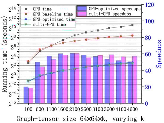
Figure 6.
Running time of the GPU-base baseline, optimized, and multi-GPU implementations and the CPU MATLAB implementation with synthetic graph-tensors of . Speedups of the GPU-optimized and multi-GPU implementations correspondingly.
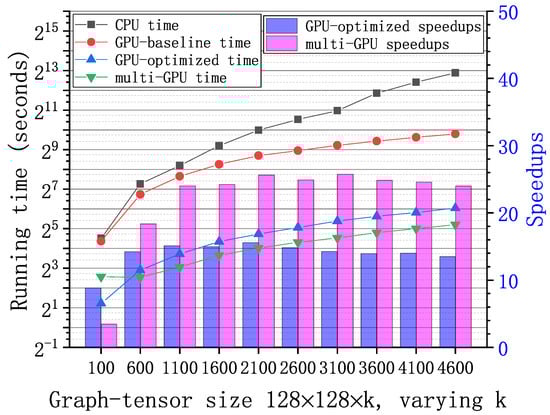
Figure 7.
Running time of the GPU-base baseline, optimized, and multi-GPU implementations and the CPU MATLAB implementation with synthetic graph-tensors of . Speedups of the GPU-optimized and multi-GPU implementations correspondingly.
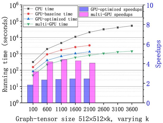
Figure 8.
Running time of the GPU-base baseline, optimized, and multi-GPU implementations and the CPU MATLAB implementation with large-scale synthetic graph-tensors of . Speedups of the GPU-optimized and multi-GPU implementations correspondingly. Graph-tensors of and larger exceed the capability of a single GPU.
Table 2.
Running time breakdown for a graph-tensor of using nvprof.
The multi-GPU scheme has two major advantages: performance improvement and supporting large-scale graph-tensors. As shown in Figure 6, Figure 7 and Figure 8, compared to the GPU-baseline implementation on a single GPU, the multi-GPU implementation achieves up to , , and speedups for graph-tensors of size , , and , respectively. Compared to the GPU-optimized implementation on a single GPU, the multi-GPU implementation achieves up to speedups. On small-scale graph-tensors, the multi-GPU implementation running on two GPUs is slightly slower than the GPU-optimized implementation running on a single GPU, as shown in Figure 6. The reason is that there is overhead introduced by data splitting and the synchronization among multiple GPUs. For medium-scale and large-scale graph-tensors, the multi-GPU implementation running on two GPUs significantly outperforms the GPU-optimized implementation running on a single GPU, as shown in Figure 7 and Figure 8. The performance improvement of computing on multiple GPUs outweighs the overhead introduced by the multi-GPU scheme. In addition, Figure 8 shows that the multi-GPU implementation can process large graph-tensors of or larger, which are not supported by the GPU-baseline or GPU-optimized implementations running on a single GPU.
Figure 9 shows the rMSE of graph-tensor imputation algorithm with synthetic data on CPU and GPUs, respectively. We set the missing rate to 20% and configure the algorithm to execute for 20 iterations with . Both the GPU implementation and the CPU implementation achieve low recovery errors in the order of (i.e., good accuracy). In addition, the rMSEs of the GPU implementation are very close to those of the CPU MATLAB implementation under different sizes of graph-tensors, which validates the correctness of the GPU implementations.
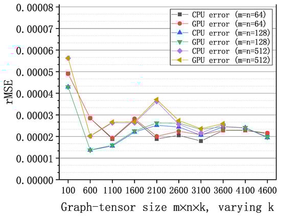
Figure 9.
The relative square errors of the algorithm with synthetic graph-tensors of different sizes on GPU and CPU, respectively.
For the graph-tensor of size generated from the real-world ego-Facebook graph [27], we vary the missing rates from 5% to 50% and evaluate the performance of algorithms. Figure 10 shows the running time and speedups of the CPU MATLAB, GPU-baseline, and GPU-optimized implementations. We can observe that as the growth of the missing rates, the recovery time also increases both on CPU and GPU. The average running time of the CPU implementation, the GPU-baseline implementation, and the GPU-optimized implementation is 1051.73 s, 522.04 s and 6.75 s, respectively. Compared to the GPU-baseline implementation, the GPU-optimized implementation achieves up to speedups.
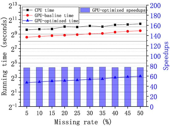
Figure 10.
Running time and speedups of the graph-tensor imputation with the ego-Facebook graph [27] under varying missing rates on GPU and CPU, respectively.
For the graph-tensor of size generated from the real-world ego-Facebook graph [27], Table 3 shows the average recovery errors of the CPU implementation and the GPU implementation under varying observing rates from to , where (i.e., the number of vertices). The rMSEs decreases with the increasing of observing rates both on CPU and GPU since fewer slices are missed in the graph-tensors. Besides, the GPU implementation achieves the same rMSEs with the CPU implementation on all observing rates.
Table 3.
Average relative mean square errors (rMSEs) under varying observing rates.
7. Conclusions
In this paper, we proposed a GPU-based convolutional imputation algorithm for high-performance and accurate graph-tensor imputation with the slice-sampling pattern. Focusing on compute-intensive GFT, iGFT, and SVD operations, we optimized memory accesses, GPU utilization, and CPU-GPU communications. By utilizing coalesced memory access, streams and batched computing, the GPU-optimized implementation achieves up to speedups over the GPU-baseline implementation with synthetic data. In addition, we designed a multi-GPU implementation to further improve performance and support large-scale graph-tensors on multiple-GPUs on a computing node. The multi-GPU implementation achieves up to speedups on two GPUs versus the GPU-optimized implementation on a single GPU. With the graph-tensors generated from the real-world ego-Facebook graph [27], the GPU-optimized implementation achieves up to speedups versus the GPU-baseline implementation. Besides, the GPU implementation and CPU implementation achieve similar, low recovery errors. In the future, we plan to scale this work onto multi-node GPU clusters to support wider applications.
Author Contributions
Abstract, introduction, related works, conclusions, and the revising of the entire manuscript, T.Z.; algorithms, experiments, and results, C.Z. All authors have read and agreed to the published version of the manuscript.
Funding
This research is partially supported by Science and technology committee of Shanghai Municipality under grant No. 19511121002.
Data Availability Statement
Not Applicable.
Acknowledgments
The authors would like to thank anonymous reviewers for their fruitful feedback and comments that have helped them improve the quality of this work.
Conflicts of Interest
The authors declare no conflict of interest.
References
- Liu, X.Y.; Wang, X. LS-decomposition for robust recovery of sensory big data. IEEE Trans. Big Data 2018, 4, 542–555. [Google Scholar] [CrossRef]
- Sun, Q.; Yan, M.; Donoho, D. Convolutional Imputation of Matrix Networks. In Proceedings of the International Conference on Machine Learning, Stockholm, Sweden, 10–15 July 2018; pp. 4818–4827. [Google Scholar]
- Liu, X.Y.; Aeron, S.; Aggarwal, V.; Wang, X. Low-tubal-rank tensor completion using alternating minimization. IEEE Trans. Inf. Theory 2019, 66, 1714–1737. [Google Scholar] [CrossRef]
- Zhang, T.; Liu, X.Y.; Wang, X. High Performance GPU Tensor Completion with Tubal-sampling Pattern. IEEE Trans. Parallel Distrib. Syst. 2020, 31, 1724–1739. [Google Scholar] [CrossRef]
- Liu, X.Y.; Zhu, M. Convolutional graph-tensor net for graph data completion. In IJCAI 2020 Workshop on Tensor Network Representations in Machine Learning; Springer: Berlin/Heidelberg, Germany, 2020. [Google Scholar]
- Kyrola, A.; Blelloch, G.; Guestrin, C. Graphchi: Large-scale graph computation on just a PC. In Proceedings of the 10th USENIX Symposium on Operating Systems Design and Implementation (OSDI 12), Hollywood, CA, USA, 8–10 October 2012; pp. 31–46. [Google Scholar]
- Wang, Y.; Davidson, A.; Pan, Y.; Wu, Y.; Riffel, A.; Owens, J.D. Gunrock: A high-performance graph processing library on the GPU. In Proceedings of the 21st ACM SIGPLAN Symposium on Principles and Practice of Parallel Programming, Barcelona, Spain, 12–16 March 2016; pp. 1–12. [Google Scholar]
- Dathathri, R.; Gill, G.; Hoang, L.; Dang, H.V.; Brooks, A.; Dryden, N.; Snir, M.; Pingali, K. Gluon: A communication-optimizing substrate for distributed heterogeneous graph analytics. In Proceedings of the 39th ACM SIGPLAN Conference on Programming Language Design and Implementation, Philadelphia, PA, USA, 18 June 2018; pp. 752–768. [Google Scholar]
- Perraudin, N.; Paratte, J.; Shuman, D.; Martin, L.; Kalofolias, V.; Vandergheynst, P.; Hammond, D.K. GSPBOX: A toolbox for signal processing on graphs. arXiv 2014, arXiv:cs.IT/1408.5781. [Google Scholar]
- Defferrard, M.; Martin, L.; Pena, R.; Perraudin, N. Pygsp: Graph Signal Processing in Python. 2017. Available online: https://github.com/epfl-lts2/pygsp (accessed on 31 January 2021).
- Gori, M.; Monfardini, G.; Scarselli, F. A new model for learning in graph domains. In Proceedings of the 2005 IEEE International Joint Conference on Neural Networks, Montreal, QC, Canada, 31 July–4 August 2005; Volume 2, pp. 729–734. [Google Scholar]
- Wu, Z.; Pan, S.; Chen, F.; Long, G.; Zhang, C.; Philip, S.Y. A comprehensive survey on graph neural networks. IEEE Trans. Neural Netw. Learn. Syst. 2020, 32, 4–24. [Google Scholar] [CrossRef] [PubMed]
- Estrach, J.B.; Zaremba, W.; Szlam, A.; LeCun, Y. Spectral networks and deep locally connected networks on graphs. In Proceedings of the 2nd International Conference on Learning Representations ICLR, Banff, AB, Canada, 14–16 April 2014. [Google Scholar]
- Adomavicius, G.; Kwon, Y. Multi-Criteria Recommender Systems; Springer: Boston, MA, USA, 2015; pp. 847–880. [Google Scholar]
- Li, X.; Ye, Y.; Xu, X. Low-rank tensor completion with total variation for visual data inpainting. In Proceedings of the Thirty-First AAAI Conference on Artificial Intelligence, San Francisco, CA, USA, 4–9 February 2017; pp. 2210–2216. [Google Scholar]
- Liu, J.; Musialski, P.; Wonka, P.; Ye, J. Tensor Completion for Estimating Missing Values in Visual Data. IEEE Trans. Pattern Anal. Mach. Intell. 2013, 35, 208–220. [Google Scholar] [CrossRef] [PubMed]
- Zhang, T.; Liu, X.Y.; Wang, X.; Walid, A. cuTensor-Tubal: Efficient primitives for tubal-rank tensor learning operations on GPUs. IEEE Trans. Parallel Distrib. Syst. 2019, 31, 595–610. [Google Scholar] [CrossRef]
- Abdelfattah, A.; Keyes, D.E.; Ltaief, H. KBLAS: An Optimized Library for Dense Matrix-Vector Multiplication on GPU Accelerators. ACM Trans. Math. Softw. 2016, 42, 18. [Google Scholar] [CrossRef]
- Jia, Z.; Kwon, Y.; Shipman, G.; McCormick, P.; Erez, M.; Aiken, A. A distributed multi-gpu system for fast graph processing. Proc. VLDB Endow. 2017, 11, 297–310. [Google Scholar] [CrossRef]
- Zhang, T.; Lu, H.; Liu, X.Y. High-Performance Homomorphic Matrix Completion on Multiple GPUs. IEEE Access 2020, 8, 25395–25406. [Google Scholar] [CrossRef]
- Sandryhaila, A.; Moura, J.M.F. Big Data Analysis with Signal Processing on Graphs. IEEE Signal Process. Mag. 2014, 31, 80–90. [Google Scholar] [CrossRef]
- Kilmer, M.E.; Martin, C.D. Factorization strategies for third-order tensors. Linear Algebra Its Appl. 2011, 435, 641–658. [Google Scholar] [CrossRef]
- Ortega, A.; Frossard, P.; Kovačević, J.; Moura, J.M.; Vandergheynst, P. Graph signal processing: Overview, challenges, and applications. Proc. IEEE 2018, 106, 808–828. [Google Scholar] [CrossRef]
- Corporation, N. NVIDIA CUDA SDK 10.1, NVIDIA CUDA Software Download. 2019. Available online: https://developer.nvidia.com/cuda-downloads (accessed on 31 January 2021).
- Corporation, N. NVIDIA QUADRO RTX 6000. 2021. Available online: https://www.nvidia.com/en-us/design-visualization/quadro/rtx-6000 (accessed on 31 January 2021).
- Corporation, N. NVIDIA V100 TENSOR CORE GPU. 2021. Available online: https://www.nvidia.com/en-us/data-center/v100 (accessed on 31 January 2021).
- Leskovec, J.; Krevl, A. SNAP Datasets: Stanford Large Network Dataset Collection. 2014. Available online: http://snap.stanford.edu/data (accessed on 31 January 2021).


Publisher’s Note: MDPI stays neutral with regard to jurisdictional claims in published maps and institutional affiliations. |
© 2021 by the authors. Licensee MDPI, Basel, Switzerland. This article is an open access article distributed under the terms and conditions of the Creative Commons Attribution (CC BY) license (http://creativecommons.org/licenses/by/4.0/).