Abstract
Nowadays there are many DNS firewall solutions to prevent users accessing malicious domains. These can provide real-time protection and block illegitimate communications, contributing to the cybersecurity posture of the organizations. Most of these solutions are based on known malicious domain lists that are being constantly updated. However, in this way, it is only possible to block malicious communications for known malicious domains, leaving out many others that are malicious but have not yet been updated in the blocklists. This work provides a study to implement a DNS firewall solution based on ML and so improve the detection of malicious domain requests on the fly. For this purpose, a dataset with 34 features and 90 k records was created based on real DNS logs. The data were enriched using OSINT sources. Exploratory analysis and data preparation steps were carried out, and the final dataset submitted to different Supervised ML algorithms to accurately and quickly classify if a domain request is malicious or not. The results show that the ML algorithms were able to classify the benign and malicious domains with accuracy rates between 89% and 96%, and with a classification time between 0.01 and 3.37 s. The contributions of this study are twofold. In terms of research, a dataset was made public and the methodology can be used by other researchers. In terms of solution, the work provides the baseline to implement an in band DNS firewall.
1. Introduction
The DNS is a fundamental service to the functioning of the Internet. Name servers maintain the mapping between a logical name and the IP address of the servers, so that all communications start by contacting the DNS to obtain the IP address before accessing the desired service (All abbreviations have been listed in Abbreviations Section).
As the Internet grows, so does the number of DNS domains. According to the report provided by Verisign [1], the second quarter of 2020 closed with 370.1 million new domain name registrations across all TLD. An increase of 0.9 percent when compared to the first quarter of 2020, and an increase of 4.3 percent, year over year. Unfortunately, this growth has a less positive side. In [2] it is said that 70% of 200,000 newly registered domains every day are malicious or suspicious. According to the same study, these new domains stay active only for a very brief period, just hours, while others are quickly spotted behaving as command and control servers or distributing malware or phishing attacks.
Most of the current DNS firewall solutions are based on blocklists of malicious domains. When a request is sent to these systems, it is filtered and a query is produced to check the veracity of the domain. The blocklists are constantly updated, but if a new malicious domain is not yet in the list the request continues the flow without any filter, leaving the user/organization exposed to potential cyberattacks. Another approach to malicious domain detection is passive DNS analysis. This method consists of the analysis and exploration of DNS logs to find patterns and extract valuable information in order to detect malicious domain names. In [3], the author collected and analyzed real-world DNS data to detect malicious behavior and was able to detect different patterns, such as unauthorized name servers and botnet controllers. Furthermore, based on passive DNS analysis, the study [4] focuses on the passive analysis of recursive DNS traffic traces collected from multiple large networks. The authors analyzed more than 2500 million DNS queries, and were able to accurately detect malicious flux service networks (multiple IP addresses per malicious domain name that changes in quick succession to difficult take-down operations).
Considering the number of malicious domains and their short lifetime, the filtering based on blocklist and passive DNS analysis is not enough to mitigate the problems. To cope with the challenge of detecting attempts to communicate with malicious domains in a timely manner, we propose the study and implementation of a DNS firewall solution based on ML. There are previous studies that also detect malicious domains on the fly, such as [5,6,7]. However, as described in the next sections, we will explore a different approach in order to detect malicious domains with high accuracy rates and in a timely manner. Our approach considers a set of steps, all of them important, namely:
- Due to the non-existence of a DNS dataset, a list of malicious and non-malicious domains needs to be selected;
- From the list of domains, other features that can add value to the analysis should be derived. This process consists of data enrichment and involves the use of OSINT sources;
- The resulting dataset must be analyzed and prepared before it is submitted to ML algorithms. This step includes an exploratory data analysis to ascertain the existence of missing data and extreme values. It also involves the processing of data in order to obtain a dataset that can be analyzed using ML algorithms;
- The ML algorithms should be selected according the type of analysis to be done (e.g., supervised versus unsupervised learning);
- The features importance should be accessed to maximize the accuracy while reducing the time to classify the domain names;
- Different experimental analysis should be conducted to determine which algorithm(s) is most suitable for further use;
- Conclusions should be drawn on the effectiveness of the solution and on its possible use in in-band or out-band mode to detect and mitigate problems related to communication with malicious domains.
The creation of a DNS Firewall capable of detecting and blocking malicious communications in an accurate and timely manner is very important. Since the DNS is the basis for establishing communications, detecting and interrupting malicious communications at their source, independently from the attack vector, will prevent the escalation of cyber-attacks, thus protecting organizations from the economic and reputation damages associated with this kind of attack. The novelty of this study regards the custom-created dataset as well the methodology adopted. The combination of those factors allowed us to reach high accuracy rates in a timely manner to identify malicious domains. Compared to previous studies mentioned in the literature section, our results stand out by the use of a small sized dataset to train the ML models, which were able to reach high score rates. Furthermore, results from the use of six different ML algorithms provides a comparison that can be explored by other researchers.
This article is organized as follows: Section 2 describes the work carried out by other researchers. Section 3 presents the proposed methodology to implement the DNS firewall solution. Section 4 focuses on the DNS dataset creation and analysis. Section 5 presents the data analysis through data preparation, ML classification models used on this work, and the results. Section 6 presents the experimental results and Section 7 provides the discussion of the results. Section 8 concludes the paper.
2. State of the Art
The DNS is the central element of the internet and a widely know entry point for cyber-attacks. According to International Data Corporation’s 2020 threat report [8], almost 80% of cybersecurity issues involve a malicious DNS query. Also in the cybersecurity context, the last Global DNS Threat Report [9] found that, globally, 87% of the surveyed organizations suffered from cyber-attacks, with an average cost of 779,008€.
The DNS is responsible for mapping domain names to an IP address and to make use of a caching system to store a domain name with a defined ttl1. Nowadays, millions of devices are using DNS servers to be able to navigate on the internet. The DNS servers communication are made in unique and unsigned packets [10], making these a target for attackers. According to [11], there are numerous vulnerabilities related to the DNS, such as man-in-the-middle attacks, packet sniffing, transaction ID guessing, caching problems, cache poisoning, and DDOS attacks. Some threats, such as phishing attacks and malware installation, might depend on a DNS request [12] either to establish a communication between a victim and the command and control server, or to simply create a malicious domain to promote malware dissemination and data theft. Therefore, there is a need to improve DNS security to ensure secure DNS communications.
Motivated by the many vulnerabilities and a historical record of attacks on DNS systems, two major security improvements were made: the use of DNSSEC and the DNS firewall solutions.
The DNSSEC is related to several RFC such as the RFC 4033 [13] a standard is established to add data origin authentication and data integrity to the DNS using cryptographic digital signatures based on public-key cryptography. The DNSSEC exists for a long time and 90% of the TLD has the DNSSEC implemented and enabled [14], but according to [15] “only 1% of the .com, .org, and .net domains attempt to deploy DNSSEC”. According to [16], the DNSSEC provides protection against spoofing of DNS data, and also to man-in-the-middle attacks, by adding a layer of authentication to the traditional DNS. There is some complexity in the implementation of a DNSSEC solution, as mentioned in [17]. This complexity can lead to a bad configuration which can result in vulnerabilities in the DNSSEC server. In [18] the authors gathered 282,766 domain names and 4% of the domains with DNSSEC implemented showed a form of misconfiguration. According to [11] there are some different vulnerabilities to the DNSSEC, such as the chain of trust (root public key injection), security considerations for key management, key rollovers, zone private key storage, and DNSSEC timing issues.
In the DNS firewall solutions context, one of the current challenges is the use of DGA by malicious actors. According to [19], there are four methods in which the DGA are based: arithmetic, hash, wordlist and permutation. These methods take a seed as an input, output a string, and append a TLD. Due to the randomness of these domains, it is difficult to determine if a given domain name is malicious or not. In [20], a ML framework is proposed to identify DGA domain names based on deep neural networks. The results are encouraging, reaching 98.7% on average for the F1 score, and a precision of 83%. With a ML model trained to detect malicious domains, created using DGA methods or not, it is a valuable complement to actual firewall systems. In [5], the authors proposed the EXPOSURE, a system that employs passive DNS analysis techniques to detect malicious domains. They built a classifier model based on Decision Tree algorithm (J48), working in real-time, over 15 features and reaching 98% of accuracy on a 10 fold cross-validation analysis. Another DNS based approach is proposed in [6] and combines the domain features, host-based features, and web-based features to identify malicious domains. Using a small set of domains (10,000), the authors could reach 60% accuracy, which can be certainly improved when applied to larger datasets.
Regarding the used dataset, there are some related works about the creation process. In [21], the authors collected more than 100 numerical features of a domain. The collected data were based on DGA and legitimate domain names to provide a large dataset to the scientific community. The lack of features from OSINT sources are a potential limitation that we took into account in our dataset creation process. Contrarily, in [22] the authors collected around 1.5 million domain names and extracted 11 features mainly based on host-based and web-based characteristics of a domain, such as the IP address, TLD and information from WHOIS, but not using numerical features. Therefore, we create a dataset with 34 features using numerical, host-based, and web-based characteristics of a domain name.
Although there are numerous studies on DNS firewall systems, the need to analyze and predict newly malicious domains over DNS communications in a timely manner is a valuable cybersecurity countermeasure to mitigate, prevent and alert both organizations and end-users against malicious DNS traffic.
3. Proposal and Methodology
A DNS firewall system as we propose can be used to complement the DNS firewall systems based on block/allow lists with a ML model capable of verifying if a domain is malicious or not. In this way, it is possible to block access to domains that are already recognized as malicious and to others that are not yet catalogued as such, but which have a high probability of being so.
The proposed firewall solution will be built in two distinct operation modes: in-band and out-band. The in-band mode makes use of active DNS analysis and the out-band mode follows the passive DNS analysis approach as described below:
- In-band: As illustrated in Figure 1, for the in-band mode, the DNS resolution requests are analyzed in real time. This allows the determination of whether the requested domain is malicious or not and blocks or alerts as soon as possible to the fact. The overhead introduced by the DNS firewall is important and will be addressed in the analysis considering different DNS request workloads.
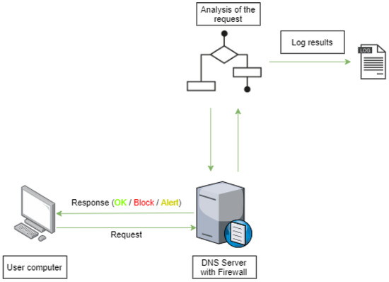 Figure 1. DNS Firewall operating in In-band.
 - Out-band: As illustrated in Figure 2, in the out-band mode the DNS firewall will only periodically analyze the DNS log. This way it will only be able to provide a posterior analysis. Thus, it is useful to identify devices within the network that are involved in malicious communications. This operation mode does not introduce overhead to the normal processing of DNS requests.
 Figure 2. DNS Firewall operating Out-band.
The analysis of the two modes of operation is very important as it allows the effectiveness of the solution to be evaluated, and its behavior to be measured in a real-time operation mode.
The main operation mode is illustrated in Figure 3. The system will analyze each DNS query to gather information about the domain name and use that information as input for posterior processing. In this step, parameters such as the WHOIS information (a record listing about entities on the internet), IP address, and subdomains will be collected. After the parameters collection, the data will be sent to a ML classification algorithm already trained. The classification response will be used to determine if the domain is malicious or not (considering the algorithm accuracy).

Figure 3.
DNS query flowchart.
The data analytics process involves several stages, namely: data collection; exploratory analysis; data preparation and ML algorithms evaluation (including feature selection and classification).
In the data collection step, random domain names collected from publicly available data sources and already classified as malicious or non-malicious, will be processed. For each domain name, parameters such as the WHOIS information and the entropy of the domain name will be extracted. In the exploratory analysis, the data collected will be analyzed, taking into account factors such as the correlation of malicious and non-malicious for each parameter, the count of “null” values and the geographic distribution. The data preparation is a crucial step to structure, clean and adapt data to be consumed by ML algorithms. It requires the transformation of non numeric data into numeric using well-known methods such as label encoding, fitting of the numeric parameters with high variance into a predefined scale, and standardization of the “null” values. Finally, the ML algorithms evaluation involves two sub-steps: feature selection and classification. In the selection of features, algorithms will be used to obtain the importance of each parameter and exclude the ones with less relevance to avoid the over-fitting problem. The classification is the last sub-step that will make use of the predefined selected features and evaluate, for each ML algorithm, its accuracy, precision, F1 score, and classification time.
The process of the DNS dataset creation to be used to train ML algorithms and choose the best ML algorithm from a historical set of DNS requests is presented in the next section.
4. DNS Dataset
In this section, the DNS dataset creation process is presented. The data collection for non-malicious domains was based on DNS logs, and uses four types of records (A, AAAA, CNAME and MX). The domains were collected from Rapid7 Labs [23], which provide datasets of DNS requests from their Project Sonar. This data are open and provide a structured schema that facilitates the extraction process. A total of 45,000 domains were randomly selected from these lists.
The malicious domains were collected from the SANS [24] public list. This list contains malicious domains validated using common publicly available virus detectors. A total of 45,000 domains were randomly selected from the list.
A total of 90,000 domain names constitutes the entry point to the information gathering process using OSINT sources. To do so we implemented a DNS configuration and submitted each name to the resolver. This way we recreate the process as it really is. The DNS server output is used as input for a Python application that processes the domain name and enriches it with useful information. As the output, a CSV file is created. The last column is named “Class” and it is the dependent variable classifying each domain as malicious or non-malicious. The dataset is composed of thirty-four features per DNS domain name:
- Domain–Baseline DNS used to enrich data, e.g., derive features;
- DNSRecordType–DNS record type queried;
- MXDnsResponse–The response from a DNS request for the record type MX;
- TXTDnsResponse–The response from a DNS request for the record type TXT;
- HasSPFInfo–If the DNS response has Sender Policy Framework attribute;
- HasDkimInfo–If the DNS response has Domain Keys Identified Email attribute;
- HasDmarcInfo–If the DNS response has Domain-Based Message Authentication;
- IP–The IP address for the domain;
- DomainInAlexaDB–If the domain is registered in the Alexa DB;
- CommonPorts–If the domain is available on common ports (21, 22, 23, 25, 53, 80, 110, 143, 161, 443, 445, 465, 587, 993, 995, 3306, 3389, 7547, 8080, 8888);
- CountryCode–The country code associated with the IP of the domain;
- RegisteredCountryCode–The country code defined in the domain registration process (WHOIS);
- CreationDate–The creation date of the domain (WHOIS);
- LastUpdateDate–The last update date of the domain (WHOIS);
- ASN–The Autonomous System Number for the domain;
- HttpResponseCode–The HTTP/HTTPS response status code for the domain;
- RegisteredOrg–The organization name associated with the domain (WHOIS);
- SubdomainNumber–The number of subdomains for the domain;
- Entropy–The Shannon Entropy of the domain name;
- EntropyOfSubDomains–The mean value of the entropy for the subdomains;
- StrangeCharacters–The number of characters different from [a-zA-Z] and considering the existence maximum of two numeric integer values;
- TLD–The Top Level Domain for the domain;
- IpReputation–The result of the blocklisted search for the IP;
- DomainReputation–The result of the blocklisted search for the domain;
- ConsoantRatio–The ratio of consonant characters in the domain;
- NumericRatio–The ratio of numeric characters in the domain ();
- SpecialCharRatio–The ratio of special characters in the domain;
- VowelRatio–The ratio of vowel characters in the domain;
- ConsoantSequence–The maximum number of consecutive consonants in the domain;
- VowelSequence–The maximum number of consecutive vowels in the domain;
- NumericSequence–The maximum number of consecutive numbers in the domain;
- SpecialCharSequence–The maximum number of consecutive special characters in the domain;
- DomainLength–The length of the domain;
- Class–The class of the domain (malicious = 0 and non-malicious = 1);
The process of data gathering, extraction of information and storage into a structured file is explained in [25]. The source code used, the produced dataset, and the exploratory analysis is also publicly available.
5. Data Analysis
In this section, the data preparation phase, the feature selection process and the ML algorithms adopted for the analysis are presented.
5.1. Data Preparation
According to [26], there are several tasks for preparing the data, such as data cleaning and data transformation. For the data cleaning step, all null values for text type columns were set as “null” (string data type). For the remaining column types, the null values were replaced according to that described in a previous paper available in [25] (e.g., null values have been replaced by the default value).
In the data transformation step, we ignored the Domain and DNSRecordType columns, as mentioned in [25], the Domain column was anonymized according to the GDPR rules, and the DNSRecordType was left in the dataset for filtering purposes only. Therefore, these features have no value for later use in ML algorithms. For the text and boolean type columns we use the Label Encoder from SkLearn framework [27] with a value between 0 and . The boolean values were transformed to integers (0 and 1).
All integer values (excluding the Class label) were submitted to the min-max normalization, a well-known approach used in past scientific experiments like [28,29], to export all the values to a float data type and a range between 0.0 and 1.0. According to [30], the min-max method performs a linear transformation on the original data fitting numeric values into a desired scale.
Although there are several techniques for data normalization, the one that fits best in the scope of this dataset is the “Scaling to a range” using the min-max method since we have no extreme outlier values.
The resulting CSV file does not include the Domain and DNSRecordType features. All the columns with text, boolean or integers as the datatype were normalized.
This data preparation phase is very important in a ML context. A weak approach in data preparation can lead to unwanted results that are not coherent with the dataset content. The next section presents the feature importance evaluation used to extract the most important features from the dataset (normalized). The ML classification process, considering the most significant features determined in the feature selection phase, is also presented.
5.2. Machine Learning: Classification
The ML process was divided into two steps: feature selection/importance and ML algorithm classification.
In the first step, after the normalization of the dataset, we used three different methods to assess the features that have more weight for the analysis. The feature selection process allows a better understanding of the data, better understanding of the model, and reduces the number of input features while maximizing the classification accuracy results.
There are numerous methods of feature selection/importance for different scopes. Considering the state of the art, our dataset, and type of analysis, we explored the following feature selection methods:
- Feature importance: This method uses the Extra Trees Classifier algorithm to fit and return the importance of the features;
- Univariate selection: Using a mathematical approach based on statistics this method works by picking up the best features on univariate statistical tests;
- RFE: According to [31], this method fits a model and deletes the feature (or features) with the lowest importance until the specified number of features is reached.
As described in [32], the behavior and performance of a feature selection algorithm depends strongly on the classification rule, sample size, and feature/label distribution.
The feature importance method makes use of the Extra Trees Classifier algorithm to fit and return the importance of the features. The Code Snippet 1 was used to identify the most significant features.
- Code Snippet 1: Feature Importance function
- import pandas as pd
- from sklearn.ensemble import Extra Trees Classifier
- #
- # @Parameters:
- # X−Independent variables
- # y−Dependent variable
- # feature_number−predefined number of features to be selected
- #
- def feature_importance(X, y, feature_number):model = Extra Trees Classifier ()model.fit(X, y)feat_importances = pd.Series(model.feature_importances_,index=X.columns)
- return feat_importances.nlargest(feature_number). axes [0].values
The univariate selection method selects features according to the K highest scores and with chi-squared statistics of non-negative features as input function. The chi-square method can be used to find the optimal subset of all features and to remove the ones with the lowest rank. This method was applied in similar research works, such as [33] in which the purpose was the implementation of an intrusion detection model based on the fusion of this method and the SVM ML algorithm. As shown in the Code Snippet 2, the SelectKBest from SkLearn [34] was used.
- Code Snippet 2: Univarate Selection function
- import pandas as pd
- from sklearn.feature_selection import Select K Best
- #
- # @Parameters:
- # X−Independent variables
- # y−Dependent variable
- # feature_number−predefined number of features to be selected
- #
- def univariate_selection (X, y, feature_number ):bestfeatures = SelectKBest (score_func=chi2, k=feature_number)fit = bestfeatures.fit (X, y)dfscores = pd.DataFrame (fit.score_)dfcolumns = pd.DataFrame (X. columns)featureScores = pd.concat ([dfcolumns, dfscores], axis = 1)featureScores.columns = [’Features’, ’Score’]return featureScores.nlargest (feature_number, ’Score’). Features. values
The RFE (with cross-validation) method consists of the recursive processing of smaller sets of features to gather the features with the highest importance. It needs an estimator (in this case the Decision Tree Regressor was used) that will iterate and seek for the lowest feature importance and exclude it. The recursive method stops when the number of features left is equal to the desired number of features selected. After the definition of the parameters, the model is fitted and transformed using the method transform that allows reducing X to the selected features. Similarly to the previous method, a data-frame was created to save each attribute and the associated importance. The code is presented in the Code Snippet 3.
- Code Snippet 3: RFE function
- import pandas as pd
- from sklearn.tree import Decision Tree Regressor
- from sklearn.model_selection import Stratified K Fold
- from sklearn.feature_selection import RFECV
- #
- # @Parameters:
- # X−Independent variables
- # y−Dependent variable
- # feature_number−predefined number of features to be selected
- #
- def rfe_cross_validation (X, y, feature_number):rfecv = RFECV (estimator = Decision Tree Regressor (), step = 1,cv = Stratified K Fold (1 0), verbose = 1,min_features_to_select = feature_number,;n_jobs = 4)rfecv.fit (X, y)rfecv.transform (X)dset = pd.DataFrame ()dset [’attr’] = X.columnsdset [’importance’] = rfecv.estimator_.feature_impor tances_dset = dset.sort_values (by = ’importance’, ascending = False)return dset.attr.head (feature_number).values
The identification of the most significant features is an important step in the analysis especially when the number of features is high. It is necessary to remove the features with less importance to feed the ML algorithm with only the most important features, to avoid over-fitting, to decrease the training time, and to maximize the accuracy results.
Once the most significant features are identified, the next step is the application of ML algorithms to determine the classification accuracy, precision, recall, F1 score, and the score time (seconds) achieved per algorithm.
The algorithms used for the evaluation are presented below. The ML algorithms we choose are often used in supervised machine learning classification problems, as already mentioned in the state of art.
- SVM: According to [35], the SVM “accomplishes the classification task by constructing, in a higher dimensional space, the hyperplane that optimally separates the data into two categories”. The SVM algorithm can solve both linear and non-linear problems by using a parameter named a kernel, which allows the researcher to set the more relevant mathematical function regarding the problem. According to the SkLearn documentation [36], there are four distinct kernel functions: linear, polynomial, RBF and sigmoid. According to the study [37], where an identical dataset was used and comparisons were made between the four kernel types, the precision achieved was higher when linear kernel functions were used. Therefore in this evaluation we also used the linear kernel function;
- LR: The LR algorithm is a statistical regression method based on supervised learning used for predictive analysis. It makes use of linear relationships between the independent features and the target label. According to [38], this algorithm has advantages such as simple implementation and excellent performance over linear datasets. Considering that one of the goals of this research is to have a solution capable of predicting malicious domains as close to real-time as possible, performance is a major factor for choosing the algorithm;
- LDA: According to [39] the LDA is a commonly used method to classify data based on a dimensionality reduction. The main goal of a dimensionality reduction is to delete the redundant features in a dataset while retaining the majority of the data. Although it is used for predictive analysis in classification problems, there are vast use cases for this algorithm, such as face recognition [40] and medical research [41,42];
- KNN: As mentioned by DeepAI [43] “the k-nearest neighbors algorithm, or kNN, is one of the simplest machine learning algorithms. Usually, k is a small, odd number - sometimes only 1. The larger k is, the more accurate the classification will be, but the longer it takes to perform the classification”. According to [44], the optimal value of k-nearest neighbors is different for distinct data samples. For this research, the number of the k-nearest neighbors parameter was kept as 5 (the default value adopted in the SkLearn framework) [45];
- CART: The CART term refers to Decision Tree algorithms that can be used on predictive problems to do classification and regression. For this research, the Decision Tree Classifier was used, in which, according to the SkLearn documentation [46], the main goal is “to create a model that predicts the value of a target variable by learning simple decision rules inferred from the data features”. One of the main advantages of this algorithm is the simplicity of understanding and interpretation, along with the excellent performance demonstrated in previous analyses already mentioned in the state of art;
- NB: The NB algorithms are used on supervised ML algorithms by applying Bayes Theorem. According to SkLearn documentation [47], there are three major models based on NB: Gaussian, Multinomial, and Bernoulli. The Gaussian is commonly used for classification problems. The Multinomial is more used in text classification problems and implements the NB algorithm for multinomial data. The Bernoulli method implements the NB algorithm according to multivariate data distribution mainly used for text classification. Therefore we selected the Gaussian NB model in order to classify and predict the dataset in a timely manner.
After the ML algorithms selection, the dataset was split between training and testing groups using 10-fold cross-validation which is commonly used in the state of the art from different research studies. The number of features selected was nine based on repetitive evaluations. For each feature selection algorithm previously mentioned, the output was taken into account to select the higher importance features. The time metric evaluates the mean of the prediction time, for each iteration of the cross-validation.
To run each ML algorithm, we created a function that receives the dataset containing the best nine features using each one of the three feature selection/importance methods mentioned earlier in this section. To run the cross-validation process with the dependent and independent features the cross_validate function from SkLearn [48] was used. which allows to “evaluate metric(s) by cross-validation and also record fit/score times”.
To evaluate the effectiveness of the ML models we chose common metrics as follows:
- Accuracy: The accuracy is the ratio between the correctly predicted observations versus the total number of observations;
- Precision: The precision is the ratio between the correctly predicted positive observations and the total predicted positive observations;
- Recall: The recall is the ratio between the correctly predicted positive observations and all observations in the actual class (0 or 1);
- F1 score: The F1 score is the average of precision and recall and takes into account the false positives and false negatives;
- Score time: Corresponds to the time for the test of the estimator on each cross-validation iteration.
The source code used to evaluate the feature importance and the ML algorithms is publicly available in [49].
6. Results
For consistency of results, the computational performance must be taken into account. The experiments were performed on a machine with the following characteristics:
- Processor: Intel Core i7-8565U @ 1.80 Ghz;
- Memory: SDRAM DDR4-2400 16 GB (16 GB × 1);
- Graphics Processor: Intel UHD Graphics 620;
- Storage: 512 GB PCIe Gen 3 × 4;
- -
- Read up to 3100 MB/s;
- -
- Write up to 2800 MB/s.
The results for each feature importance method are described in the Table 1, Table 2 and Table 3. As mentioned in the previous section, the test mode selected was 10-fold-cross-validation and the number of features selected was nine. The features vary for each feature selection/importance method (feature importance, univariate selection and RFE).

Table 1.
Results using the Feature Importance feature selection method.
Table 2.
Results using the Univariate Selection method.
Table 3.
Results using the RFE feature selection method.
Table 1 presents the classification results achieved when considering the features with higher importance ( ’NumericRatio’, ’ConsoantRatio’, ’NumericSequence’, ’HasSPFInfo’, ’TXTDnsResponse’, ’DomainLength’, ’VowelRatio’, ’CreationDate’ and ’StrangeCharacters’) determined using the feature importance method.
Considering the feature importance method, the ML algorithm with the highest accuracy (95%), recall (93%), and F1 score (94%) was the KNN. Although this algorithm has good results, the time to predict is above 1 s (1793), losing to the CART algorithm with a score time of 0.01 s. Furthermore, the precision was slightly higher for the CART algorithm.
Table 2 presents the results when the univariate feature selection method was used. The top nine features achieved by this method were: ’HasSPFInfo’, ’TXTDnsResponse’, ’CreationDate’, ’NumericRatio’, ’LastUpdateDate’, ’HttpResponseCode’, ’ConsoantRatio’, ’MXDnsResponse’ and ’StrangeCharacters’.
From the results presented in Table 2, the algorithm with the best result was the CART. This algorithm shows a validation accuracy of 95%, with a precision of 96%. The recall reached 94% and the F1 score 95%. The lowest score time (0.013) is shared by the CART, LDA, and NB algorithm.
Table 3 presents the results achieved by using the features with higher importance according the RFE method. The features used were: ’NumericRatio’, ’ASN’, ’DomainLength’, ’NumericSequence’, ’Ip’, ’ConsoantRatio’, ’TLD’, ’StrangeCharacters’ and ’CountryCode’.
The results presented in Table 3 also reveal that the CART algorithm is the best regarding the validation accuracy. This algorithm was able to reach 96% accuracy and 97% precision with a recall value of 94% and F1 score of 95%. The time score (0.013) was also a good result, losing only to the NB algorithm (0.012), but the difference was almost insignificant.
In order to make a comparison between the results achieved so far, a new experiment was conducted. The previous results were achieved by following a traditional and manual analysis. We now compare those results with the ones achieved by using an AutoML approach. To do this, we submitted the dataset to the TPOT [50] tool that optimizes machine learning pipelines using genetic programming. This tool takes care of the data cleaning, feature-related tasks (selection, preprocessing, and construction), ML model selection, parameter optimization, and model validation tasks. To be coherent with the previous experiments, the k-fold value was set to ten. For the remaining TPOT Classifier parameters, we keep the default values. The results are presented in Table 4.
Table 4.
Results using the AutoML optimized pipeline.
The results achieved by using AutoML are not far from the results achieved by the manual/traditional approach.
In general the results achieved so far are encouraging. They show that the algorithms are able to distinguish between benign and malicious domains with accuracy rates between 89% and 96%. Considering that the time to detect malicious domains is very important, the analysis presented also considers the time, in seconds, that each algorithm took to make the decision and calculate the mean value.
7. Discussion and Recommendations
The use of AutoML methods, which automates the pipeline for ML processes, are a valuable source of comparison with traditional and manual approaches. As shown by the results, the AutoML algorithm has chosen the CART as the best algorithm and estimators to the pipeline. As shown in Table 3, although the feature selection was made using the RFE method, we also get the highest values using the CART algorithm. The accuracy only differs by decimal values (AutoML = 0.962/CART (using RFE) = 0.961). The main difference was the hyper-parameter tuning used by AutoML to reach the highest score. The time resulting from AutoML (0.025 s) was slightly higher than our result (0.0136 s). The combination of accuracy and time are important for further implementation of the DNS firewall in a real scenario where, for instance, the highest accuracy algorithm can be devalued in favor of a better time response algorithm. Another consideration must be the feature selection methods which can be improved or even excluded depending on the chosen ML algorithm. In Table 5 is possible to analyze the comparison of the selected features for each method.
Table 5.
Features importance comparison.
The data presented in Table 5 shows that for the CART algorithm, which was the model with highest accuracy validation results and one of the fastest in the score time, the best feature selection/importance algorithms was the RFE.
Table 6 represents the comparison between the ML algorithms, dataset size and accuracy score with two similar studies mentioned in the state of art.
Table 6.
Results comparison.
The results from the study in [20] reaches a highest accuracy score of 98%. Although the accuracy differs by only 2% when compared with our result, the dataset size is considerably larger which can be a valuable point to take into account for further evaluations and improvements. The result of the study in [6] reinforces the link between the dataset size and the accuracy score. The major advantage of our study consists of the methods used, such as the data preparation with normalization and label encoding, along with the RFE method to select the most important features to feed the model and obtain 96% accuracy using a relatively small dataset. Despite the dataset size, there are also numerous factors to evaluate and analyze in order to improve the ML model, such as the hyperparameter tuning, data preparation, and feature selection processes.
The ground base to implement a DNS firewall solution based on ML is completed. As future work, we envisage the implementation in a real scenario as follows: (a) creation of a DNS proxy (which will also work as a firewall), (b) application of our ML model on each request, (c) logging of the results to a future passive analysis and (d) alert/allow/block system to inform the user. The Figure 4 describes the proposed future work.
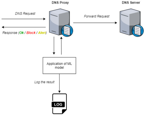
Figure 4.
DNS Proxy/Firewall.
This implementation can be a vital system when applied over a current DNS firewall without ML approaches in real-time to classify domains. The possibility to improve legacy systems is also a valuable point for users and organizations.
8. Conclusions
The main objective of our work is to implement a firewall solution based on ML in order to classify DNS requests and filter them regarding the probability of being malicious or not. The development of a DNS firewall based on ML encompasses a set of steps such as the creation of a DNS dataset from DNS logs, the exploratory analysis of the dataset, the data preparation for the ML process, the feature selection by importance and the ML algorithms application to determine the classification accuracy. To accomplish these steps, we firstly created a DNS dataset containing 34 features enriched using OSINT and analytical methods. The resulting dataset is publicly available [51] and can be used by other researchers. After this, the dataset was analyzed to correlate features with the class label providing valuable insights on how the data are distributed by malicious or benign domains. In order to be used by ML algorithms, the data were processed, making use of well known methods such as label encoding and min-max functions to normalize all the values. The feature importance process was made using three distinct methods (feature importance, univariate selection, and RFE), each one with different results. The ML algorithms were selected taking into account the type of analysis (supervised) and the state of art. Six different algorithms were used: SVM, LR, LDA, KNN, CART, and NB. The results were collected and analyzed, and we verified that the CART algorithm is the best algorithm considering the RFE feature selection method. Additionally, considering the existence of automatic ML processes, the effectiveness of this type of processes was also analyzed. We used AutoML, and a slight improvement in accuracy was observed but, as a drawback, an increase in the time to classify a set of domains was also observed.
The classification results achieved with our approach are very interesting. The results show an accuracy above 96% and a low time to classify, which is a good indicator to further explore the application and adopt it for a real scenario. The results obtained from the ML algorithms can also be used by researchers for future research in this field.
With the creation of a DNS firewall as we propose, the DNS core service is not affected. The DNS will respond to the requests, however, considering the classification result, the IP associated with the name of the request may be changed to block the connection. For example, in response to a resolution request, the DNS server may respond with the IP address 127.0.0.1, sinking the communication, thus avoiding malicious communications.
Finally, we must consider that all this work was carried out in a laboratory environment, so there is a great limitation in terms of tests in real scenario. With the creation of a prototype and testing in a real environment, we will certainly observe different results due to both the volume of orders and the variance in their characteristics. These tests will be essential to improve and make this solution more robust.
Author Contributions
C.M.: Investigation, Software, Data curation, Writing—original draft, Visualization. S.M.: Formal analysis, Writing—review & editing. J.M.: Conceptualization, Methodology, Formal analysis, Writing—review & editing. All authors have read and agreed to the published version of the manuscript.
Funding
This work was partially supported by the Norte Portugal Regional Operational Programme (NORTE 2020), under the PORTUGAL 2020 Partnership Agreement, through the European Regional Development Fund (ERDF), within project “Cybers SeC IP” (NORTE-01-0145-FEDER-000044).
Data Availability Statement
The dataset used in this study is openly available in Mendeley Data repository at 10.17632/623sshkdrz.5, version number 5.
Conflicts of Interest
The authors declare no conflict of interest.
Abbreviations
The following abbreviations are used in this manuscript:
| AutoML | Automated Machine Learning |
| CART | Decision Tree |
| CSV | Comma-separated Values |
| DDOS | Distributed Denial of Service |
| DGA | Domain generation algorithm |
| DNS | Domain Name Service |
| DNSSEC | DNS Security Extensions |
| GDPR | General Data Protection Regulation |
| IP | Internet Protocol |
| KNN | K-Nearest Neighbors |
| LDA | Linear Discriminant Analysis |
| LR | Logistic Regression |
| ML | Machine Learning |
| NB | Naive Bayes |
| OSINT | Open Source Intelligence |
| RBF | Radial basis function |
| RFC | Request For Comments |
| RFE | Recursive Feature Elimination |
| SANS | SANS Internet Storm Center |
| SVM | Support-Vector Machine |
| TLD | Top Level Domain |
| TTL | Time To Live |
References
- Verisign. The Domain Name Industry Brief. Available online: https://www.verisign.com/en_US/domain-names/dnib/index.xhtml (accessed on 28 November 2021).
- Scmagazine. Vast Majority of Newly Registered Domains Are Malicious. Available online: https://www.scmagazine.com/home/security-news/malware/vast-majority-of-newly-registered-domains-are-malicious (accessed on 9 February 2020).
- Weimer, F. Passive DNS Replication. Available online: https://static.enyo.de/fw/volatile/pdr-draft-11.pdf (accessed on 28 November 2021).
- Perdisci, R.; Corona, I.; Dagon, D.; Lee, W. Detecting malicious flux service networks through passive analysis of recursive DNS traces. In Proceedings of the Annual Computer Security Applications Conference, ACSAC, Honolulu, HI, USA, 7–11 December 2009; pp. 311–320. [Google Scholar]
- Bilge, L.; Kirda, E.; Kruegel, C.; Balduzzi, M. EXPOSURE: Finding Malicious Domains Using Passive DNS Analysis. Available online: https://sites.cs.ucsb.edu/~chris/research/docndss11_exposure.pdf (accessed on 28 November 2021).
- Palaniappan, G.; Sangeetha, S.; Rajendran, B.; Sanjay; Goyal, S.; Bindhumadhava, B.S. Malicious Domain Detection Using Machine Learning on Domain Name Features, Host-Based Features and Web-Based Features. Procedia Comput. Sci. 2020, 171, 654–661. [Google Scholar] [CrossRef]
- Segawa, S.; Masuda, H.; Mori, M. Proposal and Prototype of DNS Server Firewall with Flexible Response Control Mechanism. In Proceedings of the 20th IEEE/ACIS International Conference on Software Engineering, Artificial Intelligence, Networking and Parallel/Distributed Computing, SNPD 2019, Piscataway, NJ, USA, 8–10 July 2019; Institute of Electrical and Electronics Engineers Inc.: Piscataway, NJ, USA, 2019; pp. 466–471. [Google Scholar]
- IDC 2020 Global DNS Threat Report|DNS Attacks Defense|EfficientIP. 2020. Available online: https://www.efficientip.com/resources/idc-dns-threat-report-2020/ (accessed on 11 July 2021).
- IDC 2021 Global DNS Threat Report|Network Security. 2021. Available online: https://www.efficientip.com/resources/idc-dns-threat-report-2021/ (accessed on 22 August 2021).
- Domain Name System (DNS) Security: Attacks Identification and Protection Methods. 2018. Available online: https://csce.ucmss.com/cr/books/2018/LFS/CSREA2018/SAM4137.pdf (accessed on 22 August 2021).
- Ariyapperuma, S.; Mitchell, C.J. Security vulnerabilities in DNS and DNSSEC. In Proceedings of the Second International Conference on Availability, Reliability and Security, ARES, Vienna, Austria, 10–13 April 2007; pp. 335–342. [Google Scholar] [CrossRef]
- Anderson, C.; Conwell, J.T.; Saleh, T. Investigating cyber attacks using domain and DNS data. Netw. Secur. 2021, 2021, 6–8. Available online: https://www.sciencedirect.com/science/article/abs/pii/S1353485821000283 (accessed on 28 November 2021). [CrossRef]
- Arends, R.; Austein, R.; Larson, M.; Massey, D.; Rose, S.W. rfc4033. 2005. Available online: https://www.nist.gov/publications/dns-security-introduction-and-requirements-rfc-4033?pub_id=150135 (accessed on 22 August 2021).
- ICANN Research–TLD DNSSEC Report. Available online: http://stats.research.icann.org/dns/tld_report/ (accessed on 23 July 2021).
- Chung, T.; van Rijswijk-Deij, R.; Chandrasekaran, B.; Choffnes, D.; Levin, D.; Maggs, B.M.; Wilson, C. An End-to-End View of DNSSEC Ecosystem Management. Available online: https://www.usenix.org/system/files/login/articles/login_winter17_03_chung.pdf (accessed on 28 November 2021).
- Van Adrichem, N.L.M.; Blenn, N.; Lúa, A.R.; Wang, X.; Wasif, M.; Fatturrahman, F.; Kuipers, F.A. A measurement study of DNSSEC misconfigurations. Secur. Inf. 2015, 4, 1–14. [Google Scholar] [CrossRef]
- Antić, D.; Veinović, M. Implementation of DNSSEC-secured name servers for ni.rs zone and best practices. Serb. J. Electr. Eng. 2016, 13, 369–380. [Google Scholar] [CrossRef]
- Van Adrichem, N.L.; Lua, A.R.; Wang, X.; Wasif, M.; Fatturrahman, F.; Kuipers, F.A. DNSSEC misconfigurations: How incorrectly configured security leads to unreachability. In Proceedings of the 2014 IEEE Joint Intelligence and Security Informatics Conference, JISIC, NW, Washington, DC, USA, 24–26 September 2014; pp. 9–16. [Google Scholar] [CrossRef]
- Plohmann, D.; Yakdan, K.; Klatt, M.; Bader, J.; Gerhards-Padilla, E. A Comprehensive Measurement Study of Domain Generating Malware. In Proceedings of the 25th USENIX Conference on Security Symposium, Berkeley, CA, USA, 10–12 August 2016; USENIX Association: Berkeley, CA, USA, 2016; Volume 16, pp. 263–278. [Google Scholar]
- Ren, F.; Jiang, Z.; Wang, X.; Liu, J. A DGA domain names detection modeling method based on integrating an attention mechanism and deep neural network. Cybersecurity 2020, 3, 1–13. [Google Scholar] [CrossRef]
- Zago, M.; Gil Pérez, M.; Martínez Pérez, G. UMUDGA: A dataset for profiling algorithmically generated domain names in botnet detection. Data Brief 2020, 30, 105400. [Google Scholar] [CrossRef] [PubMed]
- Singh, A. Malicious and Benign Webpages Dataset. Data Brief 2020, 32, 106304. [Google Scholar] [CrossRef] [PubMed]
- Rapid7 Labs. Available online: https://opendata.rapid7.com/sonar.fdns_v2 (accessed on 28 November 2021).
- SANS Internet Storm Center. Available online: https://isc.sans.edu/ (accessed on 22 November 2020).
- Marques, C.; Malta, S.; Magalhães, J.P. DNS dataset for malicious domains detection. Data Brief 2021, 38, 107342. [Google Scholar] [CrossRef] [PubMed]
- Brownlee, J. Data Preparation for Machine Learning: Data Cleaning, Feature Selection, and Data Transforms in Python. Available online: https://bd.zlibcdn2.com/book/16370100/0383c0 (accessed on 28 November 2021).
- Scikit Learn. Available online: https://scikit-learn.org/stable/ (accessed on 15 September 2020).
- Srikanth Yadav, M.; Kalpana, R. Data preprocessing for intrusion detection system using encoding and normalization approaches. In Proceedings of the 11th International Conference on Advanced Computing, ICoAC 2019, Chennai, India, 18–28 December 2019; Institute of Electrical and Electronics Engineers Inc.: Chennai, India, 2019; pp. 265–269. [Google Scholar] [CrossRef]
- Sathya Durga, V.; Jeyaprakash, T. An Effective Data Normalization Strategy for Academic Datasets using Log Values. In Proceedings of the 4th International Conference on Communication and Electronics Systems, ICCES 2019, Coimbatore, India, 17–19 July 2019; Institute of Electrical and Electronics Engineers Inc.: Coimbatore, India, 2019; pp. 610–612. [Google Scholar] [CrossRef]
- Akanbi, O.A.; Amiri, I.S.; Fazeldehkordi, E. A Machine-Learning Approach to Phishing Detection and Defense. Available online: https://www.sciencedirect.com/book/9780128029275/a-machine-learning-approach-to-phishing-detection-and-defense?via=ihub= (accessed on 28 November 2021). [CrossRef]
- Recursive Feature Elimination—Yellowbrick v1.3.post1 Documentation. Available online: https://www.scikit-yb.org/en/latest/api/model_selection/rfecv.html (accessed on 2 July 2021).
- Dougherty, E.R.; Hua, J.; Sima, C. Performance of Feature Selection Methods. Curr. Genom. 2009, 10, 365. [Google Scholar] [CrossRef] [PubMed][Green Version]
- Sumaiya Thaseen, I.; Aswani Kumar, C. Intrusion detection model using fusion of chi-square feature selection and multi class SVM. J. King Saud Univ. Comput. Inf. Sci. 2017, 29, 462–472. [Google Scholar] [CrossRef]
- Sklearn.feature_selection.SelectKBest—Scikit-Learn 0.24.2 Documentation. Available online: https://scikit-learn.org/stable/modules/generated/sklearn.feature_selection.SelectKBest.html (accessed on 6 May 2021).
- Adankon, M.M.; Cheriet, M. Support Vector Machine. Available online: https://link.springer.com/referenceworkentry/10.1007%2F978-1-4899-7488-4_299 (accessed on 28 November 2021).
- 1.4. Support Vector Machines—Scikit-Learn 0.24.2 Documentation. Available online: https://scikit-learn.org/stable/modules/svm.html (accessed on 7 May 2021).
- Intan, P.K. Comparison of Kernel Function on Support Vector Machine in Classification of Childbirth. J. Mat. MANTIK 2019, 5, 90–99. [Google Scholar] [CrossRef]
- Advantages and Disadvantages of Linear Regression. Available online: https://iq.opengenus.org/advantages-and-disadvantages-of-linear-regression/ (accessed on 5 August 2021).
- Balakrishnama, S.; Ganapathiraju, A. Linear Discriminant Analysis—A Brief Tutorial. Available online: http://datajobstest.com/data-science-repo/LDA-Primer-[Balakrishnama-and-Ganapathiraju].pdf (accessed on 28 November 2021).
- Lu, J.; Plataniotis, K.N.; Venetsanopoulos, A.N. Face Recognition Using LDA-Based Algorithms. IEEE Trans. Neural Netw. 2003, 14, 195–200. [Google Scholar] [PubMed]
- Fu, R.; Tian, Y.; Shi, P.; Bao, T. Automatic Detection of Epileptic Seizures in EEG Using Sparse CSP and Fisher Linear Discrimination Analysis Algorithm. J. Med. Syst. 2020, 44, 1–13. [Google Scholar] [CrossRef] [PubMed]
- Elnasir, S.; Mariyam Shamsuddin, S. Palm Vein Recognition Based on 2D-Discrete Wavelet Transform and Linear Discrimination Analysis Big Data Review View Project Knowledge Management for Adaptive Hypermedia Learning System View Project. Available online: http://home.ijasca.com/data/documents/3_Selma.pdf (accessed on 28 November 2021).
- kNN Definition|DeepAI. Available online: https://deepai.org/machine-learning-glossary-and-terms/kNN (accessed on 22 August 2021).
- Hassanat, A.B.; Abbadi, M.A.; Altarawneh, G.A.; Alhasanat, A.A. Solving the Problem of the K Parameter in the KNN Classifier Using an Ensemble Learning Approach. Available online: https://arxiv.org/abs/1409.0919 (accessed on 28 November 2021).
- Sklearn.neighbors.KNeighborsClassifier—Scikit-Learn 0.24.2 Documentation. Available online: https://scikit-learn.org/stable/modules/generated/sklearn.neighbors.KNeighborsClassifier.html (accessed on 27 May 2021).
- 1.10. Decision Trees—Scikit-Learn 0.24.2 Documentation. Available online: https://scikit-learn.org/stable/modules/tree.html (accessed on 15 August 2021).
- 1.9. Naive Bayes—Scikit-Learn 0.24.2 Documentation. Available online: https://scikit-learn.org/stable/modules/naive_bayes.html (accessed on 12 July 2021).
- Sklearn.Model_Selection.Cross_Validate—Scikit-Learn 0.24.2 Documentation. Available online: https://scikit-learn.org/stable/modules/generated/sklearn.model_selection.cross_validate.html (accessed on 22 August 2021).
- Claudioti/Machine-Learning. Available online: https://github.com/claudioti/machine-learning (accessed on 20 August 2021).
- TPOT. Available online: http://epistasislab.github.io/tpot/ (accessed on 5 July 2021).
- Marques, C. Dataset Creator. Available online: https://github.com/claudioti/dataset-creator (accessed on 15 September 2021).
Publisher’s Note: MDPI stays neutral with regard to jurisdictional claims in published maps and institutional affiliations. |
© 2021 by the authors. Licensee MDPI, Basel, Switzerland. This article is an open access article distributed under the terms and conditions of the Creative Commons Attribution (CC BY) license (https://creativecommons.org/licenses/by/4.0/).