Article

Improving the Robustness of Model Compression by On-Manifold Adversarial Training

School of Cybersecurity, Korea University, Seoul 02841, Korea
*
Author to whom correspondence should be addressed.
Future Internet 2021, 13(12), 300; https://doi.org/10.3390/fi13120300
Submission received: 15 October 2021 / Revised: 18 November 2021 / Accepted: 23 November 2021 / Published: 25 November 2021
(This article belongs to the Special Issue Security for Connected Embedded Devices)

Abstract

:
Despite the advance in deep learning technology, assuring the robustness of deep neural networks (DNNs) is challenging and necessary in safety-critical environments, including automobiles, IoT devices in smart factories, and medical devices, to name a few. Furthermore, recent developments allow us to compress DNNs to reduce the size and computational requirements of DNNs to fit them into small embedded devices. However, how robust a compressed DNN can be has not been well studied in addressing its relationship to other critical factors, such as prediction performance and model sizes. In particular, existing studies on robust model compression have been focused on the robustness against off-manifold adversarial perturbation, which does not explain how a DNN will behave against perturbations that follow the same probability distribution as the training data. This aspect is relevant for on-device AI models, which are more likely to experience perturbations due to noise from the regular data observation environment compared with off-manifold perturbations provided by an external attacker. Therefore, this paper investigates the robustness of compressed deep neural networks, focusing on the relationship between the model sizes and the prediction performance on noisy perturbations. Our experiment shows that on-manifold adversarial training can be effective in building robust classifiers, especially when the model compression rate is high.

1. Introduction

Deep neural networks (DNNs) have achieved remarkable success with their powerful performance in various domains, such as visual recognition, natural language processing, and time-series forecasting. However, despite these achievements, the sheer size and computational requirements of running DNNs can be problematic when we deploy them in real environments, such as small IoT devices. A natural solution is to reduce the size of a DNN without hurting its prediction performance. Recent techniques on model compression follow this direction, including weight pruning [1,2,3,4,5], weight quantization [6,7], and knowledge distillation [8]. It has been reported that, using weight pruning, we can obtain sparse weight tensors removing more than 90 % of learning parameters without significant loss in accuracy [4].
However, there are emerging concerns on the robustness of DNNs on integrating DNN in security-critical application domains, such as autonomous vehicles, medical IoT devices, and smart sensors. From the works of Szegedy et al. [9] and Goodfellow et al. [10], it has been reported that a malicious adversary can generate adversarial examples, which can incur misclassification by deep neural networks, although the adversarial examples are perceptually similar to the original data points. Various methods have been proposed to exploit such a vulnerability, including the fast gradient sign method (FGSM) [10], the iterative FGSM methods [11,12,13], and the CW attack [14]. As for defense, robust optimization techniques have been suggested, including adversarial training [10,13] and TRADES [15].
Recently, Wang et al. [16] reported that, although a pruned neural network may preserve the prediction accuracy of the original neural network, it can be vulnerable to adversarial examples. Starting from this research, several studies have been conducted to solve the robustness problem of compressed models against adversarial examples [17,18,19]. Their main idea is to optimize a unified objective consisting of the adversarial training objective and the constraint for model compression.
More recently, Lee and Lee [20] introduced the robust model compression framework that uses the proximal gradient method, knowledge distillation, and adversarial training. This line of research assumes the existence of an attacker who generates so-called adversarial perturbations to induce incorrect classification. Such perturbations are likely to be off-manifold, meaning that the perturbed data points are likely to be outside of the high-density region of the data probability distribution where training and test data are sampled.
However, in an IoT environment where data acquisition can be affected by, for example, various types of sensor noise, it will be more critical to evaluate the robustness of compressed DNNs with respect to on-manifold perturbations that would happen naturally from the environment: this is the situation that we focus on in this paper. In particular, we suggest a new robust model compression method for such an environment based on the technique of on-manifold adversarial training [21,22]. Our technique makes use of on-manifold adversarial examples, which can be seen as the most difficult type of noise from the natural environment to classify correctly for a classifier. In this sense, our results can be understood as the worst-case analysis. The contributions of this paper can be summarized as follows:
  • We investigate the robustness of compressed DNN models against natural noise using on-manifold adversarial examples for the worst-case analysis, in particular at the regime of highly compressed models relevant for deploying DNNs on small embedded systems. To the best of our knowledge, there is no other work addressing this particular issue.
  • We demonstrate our idea using samples from a known probability distribution. In this setting, we can generate on-manifold adversarial examples to their mathematical definition. We also experiment with our idea using real data sets, where on-manifold adversarial examples are generated using autoencoders since we do not know the true distribution of data. In both settings, we show that on-manifold adversarial training is effective for building robust highly compressed models.
  • We also found in our experiments that on-manifold adversarial training appears to be more efficient in using model capacity than off-manifold adversarial training.

2. Related Works

2.1. Adversarial Attacks

Szegedy et al. [9] showed that an attacker can add small perturbations to input data to create adversarial examples that make a target deep neural network misclassify, without being easily detectable—we call this an adversarial attack.

2.1.1. White-Box Attacks Methods

In white-box threat models, one assumes that the attacker can acquire information about the victim model, including the model architecture, weights, learning algorithms, and hyperparameters. Szegedy et al. [9] formulated the generation of the adversarial examples as a numerical optimization problem where the 2 -norm of the perturbation is bounded (this method is often referred to as the L-BFGS attack). Goodfellow et al. [10] suggested the FGSM (Fast Gradient Sign Method), a faster method that can generate adversarial examples without a numeric solver based on the linear approximation of the objective and -norm bound of perturbations.
DeepFool [23] improved the speed of finding the minimal perturbation attacks when the number of classes is large, based on successive linearization of the classification function. The authors in [24] suggested the JSMA (Jacobian-based Saliency Map Attack), in which the contribution of each pixel to the classification outcome is evaluated, and a perturbation is generated using a minimal number of pixels: this corresponds to limiting the 0 -norm of the perturbation.
Carlini and Wagner [14] suggested a unified framework that can be used with 2 , , and 0 penalties, experimenting with different loss functions so that it can generate adversarial examples more efficiently. Meanwhile, Kurakin et al. [12] showed that adversarial examples could be implemented in physical forms, showing that adversarial attack can be a critical issue in real-world AI-based systems. Madry et al. [13] proposed an improved attack method called the projected gradient descent (PGD) attack, which is an iterative version of FGSM in its essence.

2.1.2. Black-Box Attack Methods

In black-box settings, the attacker is assumed to have no knowledge about the victim model. Still, the attacker can send input points as queries to the victim and observe the victim’s class membership or probability scores. Black-box adversarial attack methods often rely on a surrogate model trained with the attacker’s queries and the victim’s corresponding responses, using the transferability of adversarial examples from the surrogate to the victim model [25,26,27,28,29].

2.2. Defense against Adversarial Attacks

There are various existing works on defense techniques against adversarial attacks. For convenience, we divide them largely into four categories: heuristic-based, detection-based, certified defense, and adversarial training. Heuristic-based methods include defensive distillation [30], which utilizes the idea of knowledge distillation [8] to make the model less sensitive to small perturbations in input. Another example is the logit pairing [31] method that enforces logits for pairs of benign examples and their adversarial counterparts to be similar.
Detection-based defenses attempt to reject adversarial examples by detecting them. Feature squeezing [32] is a well-known method, which detects adversarial examples by comparing the model’s prediction on the original samples with that on the transformed samples, where the transformations exhibit invariance in normal samples. Metzen et al. [33] used a sub-classifier for the detection of adversarial examples, and Feinman et al. [34] detected adversarial examples based on the property that adversarial examples lie outside of a learned manifold, using kernel density estimation and uncertainty measures.
In certified defense, Raghunathan et al. [35] suggested to jointly optimize the differentiable certificate that no attack can force the error to exceed a certain threshold for a given network and test inputs. This work has been extended to use generative methods, such as VAE and GAN [36,37,38]. More recently, Zhang et al. [15] proposed a defense method named TRADES, which combines the prediction error for the adversary with the original classification error and provides an differentiable upper bound. This is one of the state-of-the-art defense mechanism against adversarial attacks.
Adversarial training (AT) is based on robust optimization [39] where the training is performed not only on the training samples but also on the worst-case adversarial examples. The early works include FGSM-AT [11], which incorporates FGSM adversarial examples during the training stage, PGD-AT [13], and curriculum adversarial training [40]. Recently, some studies have considered adversarial examples that lie on the data manifold. Ilyas et al. [37] and Song et al. [41] demonstrate that it is possible to generate adversarial examples that are the adversaries that can possibly lie on a data manifold embracing the observed data instances through manipulating the latent variable using generative models.
In the case of defense against these on-manifold adversarial examples, Stutz et al. [21] suggested on-manifold adversarial training and showed that on-manifold adversarial training boosts generalization. More recently, dual manifold adversarial training (DMAT) [42] was proposed as a defense mechanism against both on-manifold adversarial examples and off-manifold adversarial examples by combining off-manifold adversarial training and on-manifold adversarial training.

2.3. Model Compression

The basic idea of model compression is to zero out unimportant weight parameters in a neural network with a certain criterion. By removing the redundant zero weights, one can obtain a compressed model. Han et al. [1] proposed the element-wise weight pruning method to reduce the number of parameters or connections. Recently, sparse coding has been applied for model compression. These studies used 1 or 0 norm regularization to find the optimal sparse weight matrix.
Louizos et al. [5] introduced the 0 -norm regularizer as sparsity constraints. One can reduce the model weight parameters in a structured manner by group-sparse coding, where groups on a CNN can be defined filter-wise, channel-wise, or depth-wise [3,4,43,44]. In this work, we focus on the filter-wise pruning method, which makes the weight parameters in a form where it is relatively easier to construct reduced dense weight tensors.

2.4. Robust Model Compression

The robustness issue related to the model compression has been alerted by Wang et al. [16]. They argue that the pruned networks with high sparsity rates are more vulnerable to adversarial attacks. Several studies have been conducted to accomplish adversarially robust model compression. Ye et al. [17] and Gui et al. [18] proposed a unified framework for concurrent adversarial training and model pruning using the alternating direction method for multipliers (ADMM).
More recently, Sehwag et al. [19] proposed a different method that prunes weights with a criterion based on the adversarial training objective function. Madaan et al. [45] suggested that the vulnerability against adversary is caused by the distortion in the latent feature space, and they developed an adversarial neural pruning method that removes vulnerable latent-features. In the work of Lee and Lee [20], they used the proximal gradient method (PGM) and knowledge distillation for robust model compression.
Our focus is to improve the robustness of highly compressed models against natural noise, where we use the on-manifold adversarial examples as the samples with the largest noise. To the best of our knowledge, no studies have addressed this setting. Table 1 compares the existing robust DNN training methods and ours in the perspectives of model compression and on/off-manifold adversarial examples.

3. Background

Our robust model compression method is composed of model compression based on sparse coding and adversarial training based on on-manifold adversarial examples. In this section, we provide background regarding the technologies.

3.1. Model Compression Based on Sparse Coding

Suppose that f ( · ; w ) : R d R K is a classifier parametrized by the learning weight w R p , whose outcome is the scores indicating the likelihood of a given input to be each of the K classes. Given a dataset { ( x i , y i ) } i = 1 n of n input points x i R d and its labels y i { 1 , 2 , , K } , we solve the following optimization problem in sparse coding [46,47],
w * arg min w R p 1 n i = 1 n ( f ( x i ; w ) , y i ) + Ψ ( w ) ,
where ( f ( x i ; w ) , y i ) = log ( f ( x i ; w ) y i ) is the cross-entropy between the classifier’s outcome and the labels with K classes, and Ψ : R p R is a (usually) convex function used for inducing certain structure in w: a popular choice is Ψ ( w ) = λ w 1 with λ > 0 , which induces element-wise sparsity in w * [1].
In model compression, the 1 -norm based sparse coding has a practical issue in that it is difficult to determine the value of the hyperparameter λ , which corresponds to a specific compression rate. As a result, one would need to solve the above optimization problem for several values of λ ’s until he or she finds the one for the desired compression rate. Therefore, 0 -norm based sparse coding has been popular recently using Ψ ( w ) = λ w 0 where w 0 is the count of nonzero elements in w: in this case, the value of λ can be computed during optimization to achieve a specific rate of model compression [20].
Although we can set the values of unimportant weights to zero using sparse coding, this usually does not entail a reduction in memory usage and computation automatically. Since sparse tensor operations are not fast on GPUs [2], it will be better for the resulting sparse weights to have certain patterns in the locations of zero values so that we can create dense weight tensors of reduced sizes. This is the perspective taken in the filter-wise pruning method [4], where sparsity is induced by the unit of convolution filters. We can write the filter-wise pruning as a general form of group-wise sparse coding based on the 0 -norm, where we can define groups of optimization variables that will be selected or removed altogether by the mechanism:
w *   arg min w R p 1 n i = 1 n ( f ( x i ; w ) , y i ) + λ g = 1 G I [ w g 2 0 ] .
Here, λ > 0 is a hyperparameter controlling the sparsity of the model, I [ e ] represents the indicator function whose value is 1 if the statement e is true and 0 otherwise, and w g denotes the group subvector corresponding to the group indexed by g. This problem can be solved efficiently using algorithms, such as the alternating direction method for multipliers (ADMM) [17,18] and proximal gradient methods [20].

3.2. Adversarial Example

For a trained classifier f ( · ; w * ) with an optimal weight w * and an input point x, an adversarial example [9] x = x + δ is a perturbed input point such that the classification outcome of f is different between x and x , that is,
arg max k f ( x ; w * ) k arg max k f ( x ; w * ) k ,
where f ( x ; w * ) k denotes the score output for the k-th class. We often limit the size of perturbation so that δ < ϵ for a certain norm with a small ϵ > 0 , since otherwise the perturbation can be noticeable.
Although an adversarial example has constraints on the magnitude of the perturbation, it lacks constraints to remain in the data manifold, a subspace that embraces the observed examples well [21]. For this reason, we denote the adversarial examples as off-manifold adversarial examples. Here we introduce two popular methods for generating adversarial examples, namely FGSM [10] and PGD [13].

3.2.1. Fast Gradient Sign Method

The fast gradient sign method (FGSM) [10] is one of the early white-box adversarial attack methods designed to quickly find the perturbation direction in a single step so that the loss function of the target classifier increases. When the dimension of input is large, changing each feature of x by a minimum value ϵ yields a perturbation δ , δ = ϵ . This change can have a significant impact when we calculate the linear product w T x of x with the model weight vector w. Taking a first-order approximation of the target classifier’s loss function ( f ( x ; w ) , y ) to the real training example x with a small perturbation δ gives
( f ( x + δ ; w ) , y ) ( f ( x ; w ) , y ) + x ( f ( x ; w ) , y ) T δ ,
and we maximize the right-hand side for δ bounded by the norm ball of radius. This maximization of the right-hand side is exactly the same as follows:
δ = ϵ * sign ( x ( f ( x ; w * ) , y ) ) ,
where w * is the weight vector of trained target classifier. Finally, we obtain adversarial examples by adding the adversarial perturbation to the input.
x = x + ϵ sign ( x ( f ( x ; w * ) , y ) )
As the FGSM method takes only a single step to find adversarial examples, it is relatively faster than other iterative adversarial attack methods. However, this is not a sophisticated attack method since there is no process of minimizing the perceptual difference between the adversarial example x and the original input x.

3.2.2. Projected Gradient Descent

The projected gradient descent (PGD) method [13] is a powerful white-box method, which is a multi-step variant of FGSM. FGSM only can generate weak perturbation since it attempts to find optimal perturbation δ only in a single step gradient, whereas PGD can find a more powerful and effective adversary by optimizing the loss maximization problem. PGD iteratively optimizes the perturbation for n steps with a small step size of α to find more effective optimal perturbation in norm ball. In each iteration, it projects trained adversarial examples in each iteration to ϵ neighbor of the original input x. The PGD method is defined as follows:
x 0 = x , x t + 1 = Π ( x t + α sgn ( x ( f ( x t + δ ; w ) , y ) ) , δ ϵ ,
where ϵ is the bound for -norm of the perturbation δ , Π refers to the projection operation to -norm ball, and 0 < α < ϵ is the step size. PGD aims to find the neighborhood of the original vector that maximizes the loss of the target model while maintaining the size of the perturbation as minimal as possible by solving the constrained optimization problem. This is a more sophisticated approach compared to FGSM, which does not have optimization steps for finding a proper perturbation.

3.3. Adversarial Training

Adversarial training [10] is the most extensively studied defense mechanism to enhance the robustness of a DNN model against adversarial attacks based on robust optimization. The goal of robust optimization is to find a stable solution up to a certain level of uncertainty in data. To explain, let U be the uncertainty set, f ( x ; w ) denote the target classifier, and δ denote the adversarial perturbation. The assumption in adversarial training is that the perturbations to the data can be drawn from U, and the adversarial perturbations are worst-case. Among the feasible solutions, the optimal solution would be the one with the minimum loss given the worst-case realization of perturbations.
Therefore, robust optimization problems are usually formed in min-max problems, in which the objective is minimized with respect to the worst-case of perturbations. In the case of FGSM-AT, their approach is to combine both normal and adversarial examples before each training step, so that model can be trained for both normal instances and adversarial examples for robust optimization. On the other hand, PGD-AT directly perturbs the input instances and solves the min-max objective, which follows the robust optimization problem.

3.3.1. FGSM Adversarial Training

At every training iteration in FGSM-AT, it generates adversaries with FGSM, and it trains the target classifier by combining the training data with generated adversarial examples. Let f ( x ; w ) denote the trained target classifier and w is the parameter of the classifier. The objective function of FGSM adversarial training is as follows:
α ( f ( x ; w ) , y ) + ( 1 α ) ( f ( x ; w ) , y ) ,
where ( f ( x ; w ) , y ) denotes the cross-entropy loss function, and x is the adversarial example of the original input x generated by (2). α > 0 corresponds to a constant that adjusts the weight of the loss term for the original input and the adversarial example loss term, where α is generally set to 0.5 . Even though the FGSM adversarial training is a simple and effective defense method, it is known that the model produced by FGSM-AT is vulnerable to adversarial examples generated by different attack methods, such as PGD.

3.3.2. PGD Adversarial Training

Adversarial training can be described as a robust optimization problem in the following form,
min w E ( x , y ) max δ : δ ϵ ( f ( x + δ ; w ) , y ) .
In PGD-AT [13], the authors indicated a potential issue of FGSM-AT that the inner maximization in (3) may not be optimized adequately due to the use of a linearized objective function in the construction of FGSM adversarial examples. PGD-AT replaces FGSM with PGD for generating adversarial examples as the solution for the inner maximization problem. It has been shown by Madry et al. [13] that this is a better choice, resulting in more robust classifiers against adversarial attacks.

3.3.3. TRADES

TRADES [15] is a more recent robust training method against adversarial attacks. It considers the trade-off between the robustness against adversarial examples and prediction accuracy on natural samples. The basic idea of this approach is to decompose the robustness error into the natural classification error and the boundary error. The objective consists of the natural loss term for empirical risk minimization and regularization for robustness against adversarial examples. Here, the regularization term tends to push the decision boundary of the classifier away from the inputs by minimizing the distance between the prediction of the natural example f ( x ) and the prediction of the adversarial example f ( x ) .
min w E ( x , y ) ( f ( x ; w ) , y ) + β max δ : δ ϵ f ( x ; w ) , f ( x ; w ) , x = x + δ ,
where β > 0 is a balancing parameter, As in PGD-AT, TRADES generates the worst-case perturbation δ with PGD.

4. Methodology

Our main objective is to train a compressed DNN model robust to natural noise in data. This is a critical consideration for deploying DNNs in small embedded devices in IoT environments, where a small model size is desirable due to limited computation resources, and sensor noise occurrence can be relatively frequent.
However, it is not an easy task to model the noise distribution in observations without strong assumptions, for example, that noises are approximately normally distributed [48], and such an assumption may not be appropriate in all data: also, prior knowledge about the noise distribution is often not available [49]. To deal with this issue, we propose using on-manifold adversarial examples (abbreviated as adv-on, to be defined later) as the noise samples with the largest deviation. We use adv-on for two purposes:
  • To evaluate the robustness of compressed DNN models against natural noise.
  • To improve the robustness of a compressed DNN model based on sparse coding with adversarial training.
This makes a clear distinction of our work from the existing literature [17,18,19,20] on robust model compression where the robustness has been considered against (regular) adversarial examples. As discussed in Stutz et al. [21], the regular adversarial examples (generated by, for example, FGSM or PGD as discussed earlier) are likely to deviate from the data manifold—the subspace that includes natural samples well. In this sense, we regard the regular adversarial examples as off-manifold (we denote them by off-manifold adversarial examples, adv-off).

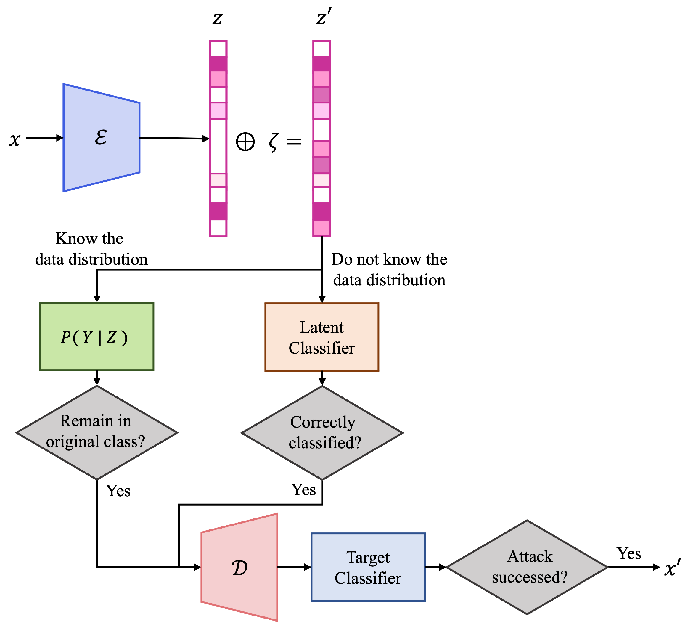
4.1. On-Manifold Adversarial Examples

An on-manifold adversarial example (denoted by adv-on) x is a perturbed version of a natural sample x that causes misclassification of the classifier, as discussed in Section 3.2. Unlike a regular adversarial example, x resides on the data manifold—in this sense, we can consider x as a natural example with noise large enough to induce incorrect classification. Adv-on’s can be formally defined as follows [21]:
Definition 1.
(On-Manifold Adversarial Example). Suppose that P is the probability distribution of data points ( x , y ) where x R d is an input and y { 1 , 2 , , K } is the corresponding true label. For a trained target classifier f : R d { 1 , 2 , , K } , an on-manifold adversarial example x of x satisfies f ( x ) y and P ( Y = y | X = x ) > P ( Y = y | X = x ) for all y { 1 , 2 , , K } \ { y } .
The definition requires that the adv-on x induces misclassification of the classifier f, but it still belongs to the original class y with respect to the data distribution P. Despite the clearness of the definition, it is not straightforward to apply it for the creation of adv-on’s since the data distribution P ( X , Y ) is typically unknown.
To circumvent the issue, we make use of the variational auto-encoder (VAE) [50] trained on natural samples. In short, the idea is to add perturbations in the latent space and then to use the decoder to generate realistic on-manifold adversarial examples. We describe our method in two cases. In the first case, we know P ( Y | Z ) where Y { 1 , 2 , , K } is the class label and Z is the random variable describing the latent space of the VAE. The second case is for real datasets where we have no access to P ( Y | Z ) , and therefore we estimate it by an auxiliary classifier. The overall process is depicted in Figure 1.

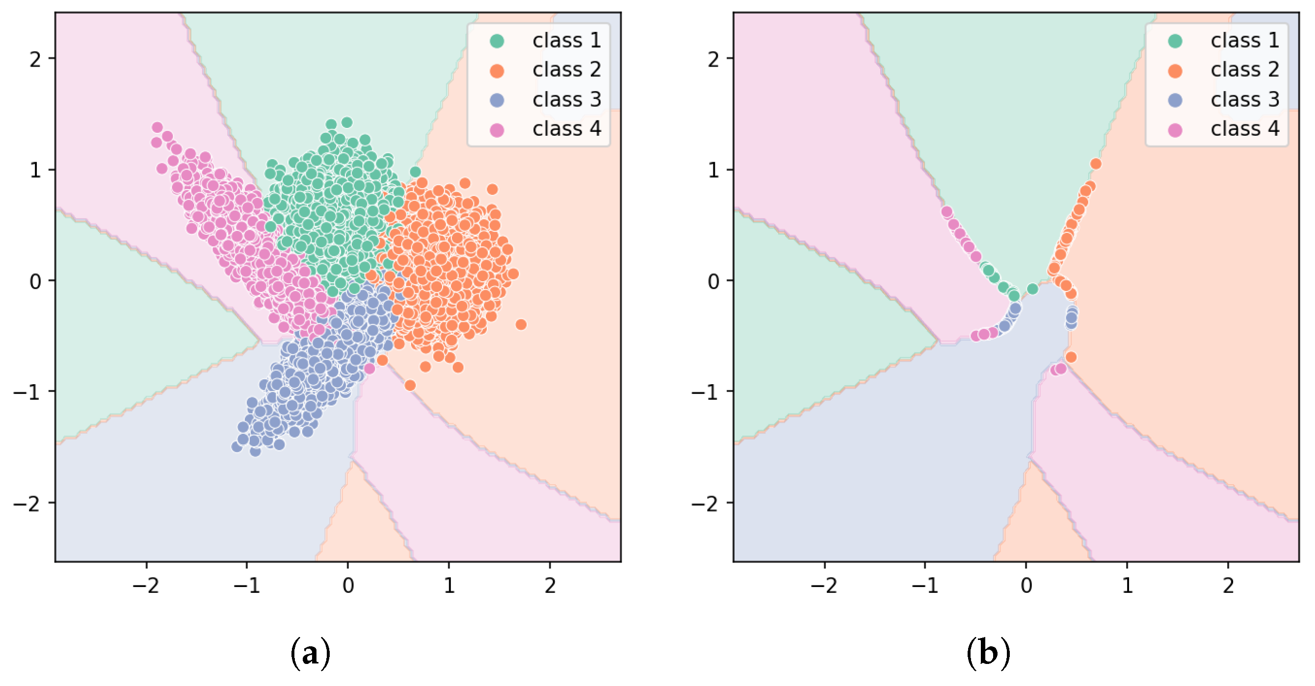
4.1.1. Case One: Simulation Data

In the case of simulation, we can define the data distribution, in particular, P ( Y | X ) to check the Definition 1. As we like to make our procedure for case one as a basis for case two below, we assume that we know P ( Y | Z ) instead of P ( Y | X ) , where Z is the random variable belonging to the latent space between an encoder E and a decoder D (to be described more in detail later). Using Baye’s rule and the transformation of random variables through X = D ( Z ) , we can establish the following connections:
P ( Y = y | Z ) = P ( Z | Y = y ) P ( Y = y ) P ( Z ) = P ( Z | Y = y ) det ( X D 1 ( X ) ) P ( Y = y ) P ( Z ) det ( X D 1 ( X ) ) P ( D 1 ( X ) | Y = y ) det ( X D 1 ( X ) ) P ( Y = y ) P ( D 1 ( X ) ) det ( X D 1 ( X ) ) = P ( X | Y = y ) P ( Y = y ) P ( X ) = P ( Y = y | X )
where P ( X ) = P ( D 1 ( X ) ) det X D 1 ( X ) is the result of transformation of the random variable X = D ( Z ) [51], and det X D 1 ( X ) is the determinant of the Jacobian of D 1 regarding X. In the approximation (the second line), we assumed that D 1 ( X ) E ( X ) = Z . The connection in (5) allows us checking the Definition 1, in particular if a perturbed point x = D ( z ) belongs to the manifold of Y = y in the space of Z, that is,
P ( Y = y | z ) > P ( Y = y | z ) , y y , and f ( D ( z ) ) y .
For simulation, we define P ( X | Y = y ) to be a two-dimensional multivariate Gaussian distribution for each of the four classes y { 1 , 2 , 3 , 4 } . To map the latent samples z R 2 to the input space (we define the input space to be sixteen-dimensional), we use a simple auto-encoder composed of two fully connected layers in the encoder E and the decoder D . The auto-encoder is trained to minimize the reconstruction error of the latent samples z (we used 17,500 samples in the experiments):
min w E , w D E z E w E ( D w D ( z ) ) z 2 2 .
With the trained decoder, we can generate on-manifold adversarial examples according to the Definition 1 using (6) (we used 70,000 generated adv-on examples as simulation data in the experiments). After generating the simulation dataset, we split the dataset randomly into trainset with 60,000 instances and testset with 10,000 instances. We separately generate on-manifold adversarial trainset and testset. Figure 2 shows the distribution of sampled latent vectors and the on-manifold vectors, respectively.

4.1.2. Case Two: Real Data

In general, we know neither P ( Y | X ) nor P ( Y | Z ) for the given dataset. However, our discussion in case one above indicates that we can follow a similar procedure if we have a good estimate of P ( Y | Z ) .
For this purpose, we train a variational auto-encoder (VAE) [50] using a given dataset in a regular setting to reduce the reconstruction error in the input space. Let us call the encoder and the decoder of the VAE as E and D , respectively. Then, using the connection (5), we train an auxiliary classifier f z = P ^ ( Y | Z ) on the latent representation z = E ( x ) of the input points x and the original labels. Assuming P ^ ( Y = y | Z ) P ( Y = y | X ) , we can check Definition 1 using (6) as in the previous case.

4.2. Model Compression with On-Manifold Adversarial Training

Our proposal method is to combine the sparse coding technique for model compression (discussed in Section 3.1) and the PGD adversarial training (Section 3.3) using on-manifold adversarial examples (Section 4.1). Our purpose is to train compressed DNN models robust to natural noise: in particular, we are interested in a high-compression regime to produce models suitable for small computation devices.
To run our method, denoted by MC-AT(on), we prepare an on-manifold dataset { ( x i , y i ) } i = 1 m + n . First, we generate n on-manifold adversarial examples by manipulating the latent vector z. Then, we select on-manifold adversarial examples by checking Definition 1. Finally, we combine selected m on-manifold adversarial examples and n original training examples.
Using this data, we can formulate MC-AT(on) as the following 0 -norm based sparse coding problem:
MC - AT ( on ) : min w R p 1 m + n i = 1 m + n f ( x i ; w ) , y i + λ w 0 ,
where λ > 0 is a hyperparameter controlling the sparsity of the model. Algorithm 1 describes the overall process of MC-AT(on) algorithm based on the proximal gradient descent algorithm [20].
Algorithm 1 Model compression by the on-manifold adversarial training algorithm
  • Require: target classifier f with weight vector w, latent classifier f z , VAE consists of encoder E and decoder D , train dataset { ( x i , y i ) } i = 1 n where x i R d , η for norm bound of perturbation;
  •  Pre-train target classifier f: min w E ( x , y ) ( f ( x ; w ) , y )
  •  Train VAE: min w E , w D E z E w E ( D w D ( z ) ) z 2 2
  •  Train latent classifier f z : min w z E ( x , y ) ( f ( E ( x ) ; w z ) , y )
  •  Initialize on-manifold adversarial dataset: M adv - on
  •  for all ( x i , y i ) { ( x i , y i ) } i = 1 n do
  •       Compute a latent vector: z i E ( x i )
  •       Compute a perturbation: ζ i arg max ζ i f ( D ( z i + ζ i ) ; w ) , y i s . t . ζ i η
  •       Add perturbation to the latent vector: z i z i + ζ i
  •       Generate an on-manifold adversarial example: x i D ( z )
  •       if  f ( x i ) y i and f z ( z i ) = y i  then
  •            insert  ( x i , y i ) to M adv - on
  •       end if
  • end for
  • M adv - on M adv - on { ( x i , y i ) } i = 1 n
  •  Apply MC-AT(on) with (7)

4.3. Computational Cost

We also conduct computational cost analysis on Algorithm 1. Hua et al. [52] analyzed the computational cost of robust training. In the case of PGD adversarial training, let P N denote the perturbation generation with N step by solving max δ : δ ϵ ( f ( x + δ ; w ) , y ) . The result of the computational complexity of adversarial training is about N times the normal DNN training. However, in our case, if we let the computational cost of training the target classifier, VAE, and latent classifier be T before crafting the latent perturbation, the total cost of training would be 3 T . After that, we craft on-manifold adversarial examples with N steps. Therefore, the total cost of generating an on-manifold adversary is 3 T + N , whereas PGD adversarial training is T × N . The adversarial training time can be improved, for example, using techniques in [53] or in [54].

5. Experiments

5.1. Datasets and Models

To investigate the effectiveness of our proposed method, we conducted experiments with different datasets. Details on the dataset and the target classifier for each dataset are described below.
  • Simulation dataset: the simulation data described in Section 4.1.1, in which on-manifold adversarial examples have been generated based on known data distribution. The simulation dataset consists of 70,000 instances with 16-dimensional inputs belonging to four different classes. We used the modified LeNet5 [55] as the classifier, which consists of two convolutional layers with max-pooling ( 5 × 5 kernel size; 32, 64 channels for simulation dataset; 64, 128 channels for MNIST), and two fully connected layers.
  • MNIST [56]: the dataset for handwritten zip-code digit classification problem, originally intended for the faster distribution of physical mail in the US post offices—the images were taken with low-resolution ( 28 × 28 ) camera sensors. This dataset consists of 70,000 grey-scale images, and the train/test split ratio is 6 : 1 . For the target classifier, we used the same model as in the simulation dataset with three fully connected layers.
  • Fashion-MNIST [57] (FMNIST): FMNIST consists of 10 different categories of fashion product images. It also includes 70,000 grey-scale images, and the train/test split ratio is 6 : 1 . We used a CNN with three convolutional layers ( 4 × 4 kernel size; 32, 64, 128 channels) and three fully connected layers.
  • CIFAR-10 [58]: CIFAR-10 consists of 60,000 RGB-color images, and the train/test split ratio is 5 : 1 . For the classifier, we used ResNet-18 [59].
  • UCI human activity recognition [60] (HAR): HAR dataset consists of nine embedded sensors and data from accelerometers and gyroscopes in smartphones. The task of the dataset is to classify six different human activities with the sensor data received from smartphones. There is a total of 10,299 instances, and we used a train/test split ratio of 7 : 3 . For the classification problem, we adopted a one-dimensional convolutional neural network model with three convolutional layers and three fully connected layers.

5.2. Methods

We compared model compression methods in five different training settings: regular model compression with no adversarial training ((1), denoted by MC(regular)); model compression with off-manifold adversarial training ((3), denoted by MC-AT(off)); on-manifold adversarial training ((7), denoted by MC-AT(on)); dual adversarial training ((3) and (7), denoted by MC-AT(dual)); and TRADES ((4), denoted by MC-TRADES).
In the case of MC-AT(dual), it is similar to Lin et al. [42], incorporating both off-manifold adversarial examples and on-manifold adversarial examples during training. We pre-trained target classifiers with the original trainsets before applying robust model compression methods. The optimization of each model compression method with adversarial training has been done with the proximal gradient method [20].

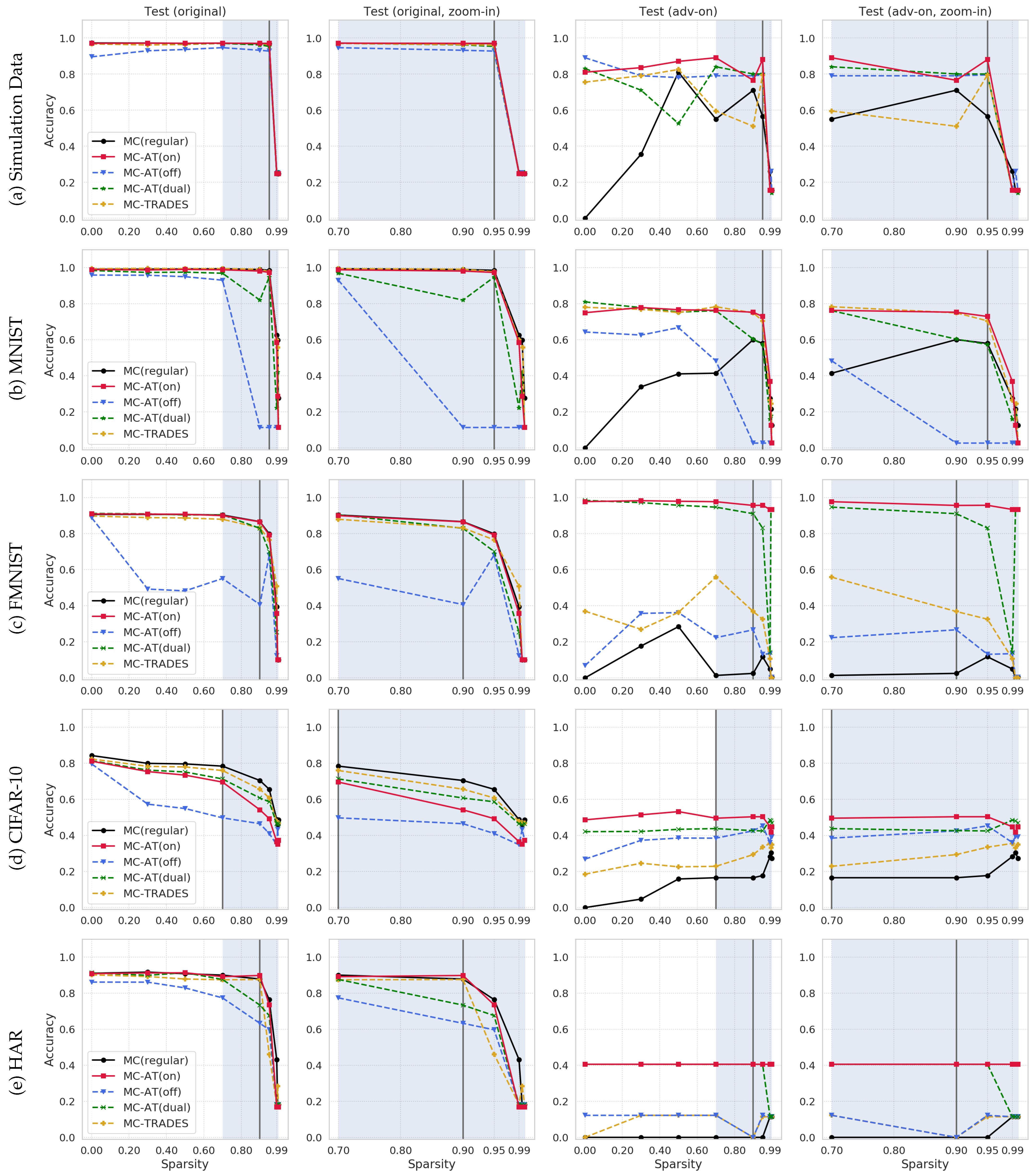
5.3. Robustness of Compressed Models on On-Manifold Test Data

We investigate the robust optimization with adv-on, which we consider as the worst-case of natural noise that can enhance the robustness of model compression.
Figure 3 shows the robustness results in terms of the prediction accuracy on the original test and adv-on test datasets. The grey vertical lines indicate the compression rate values for which the compressed models will have at least 90 % of the uncompressed reference models obtained by MC(regular). The results support our hypothesis at high compression ratios over 70 % (the area marked with blue background color in the plots): MC-AT(on) has an average performance improvement of 33.76 % on adv-on test data compared to the MC(regular).
Compared to MC-TRADES, our MC-AT(on) showed 23.68 % higher average accuracy on adv-on test. In addition, at high compression ratios over 70 % , MC-AT(on) reached 26.24 % higher average accuracy than MC-AT(off), and 10.74 % higher than MC-AT(dual). Interestingly, in the case of the HAR dataset, which is an IoT sensor dataset containing a relatively large amount of noise, only MC-AT(on) and MC-AT(dual) worked properly in the adv-on test.
Table 2 shows the comparison of robustness at the compression rates where the reduced models exhibit at least 90 % of the reference models (also indicated with grey vertical lines in Figure 3). In particular, for the combined test composed of natural test and adv-on test data, MC-AT(on) consistently showed the highest performance compared to the other robust model compression methods.
From the above results, we can conclude that MC-AT(on) can produce highly compressed DNN models robust to natural noise.

5.4. Robustness of Compressed Models on Off-Manifold Adversarial Test Data

Figure 4 shows our evaluation of the five robust model compression methods against the adv-off test data. Since the goal of our study is to present a model compression method that can enhance the robustness against noises that may exist on the data manifold, which embraces observed data well, we briefly describe the adv-off test results. Overall, MC-TRADES showed improved robustness against adv-off on average from 7.82 % to 13.06 % at high compression rates ( 70 % or more) compared to other methods.
From the results, MC-TRADES and MC-AT(dual), which are model compression methods with adversarial training that consider adv-off, showed robustness against noise that left the manifold, that is, adv-off. Therefore, it can be said that MC-TRADES and MC-AT(dual) methods are more valid for model compression for robustness against adv-off when compared with other methods.

6. Discussion

Our results show that MC-AT(on) can improve the robustness of compressed DNNs against noise-induced perturbations that may exist when collecting real-world data. The results of MC-AT(on) showed better robustness against on-manifold perturbations compared to other model compression methods in on-manifold adversarial tests. In particular for the combined accuracy on both the original test and on-manifold adversarial test, MC-AT(on) showed the highest in all five datasets, meaning that compressing a model with MC-AT(on) can develop an optimal compressed model with robustness against noises that reside on a data manifold that embraces the observed data instances.
However, our results are based on the two approximations, namely in (5) and in the use of an auxiliary classifier P ^ ( Y | Z ) to approximate the unknown distribution P ( Y | Z ) . Although the assumptions are not unlikely, the quality of approximation may vary depending on several factors, such as the dimension and number of data points, the variance of the noise, and the quality of the en/decoders. Therefore, it can be dangerous to blindly apply our proposed method, especially when these factors of one’s application data are different from our experiment settings.
On the other hand, our results also indicate that knowledge of the sensor’s noise characteristics would help to improve the classification performance when learning small neural networks. Therefore, it will be desirable for the manufacturers to provide such information and the experimenters to perform extended data analysis on the noise component in the collected IoT data.
It was a rather unexpected discovery in the HAR dataset experiment that MC-AT(on) was able to produce a more robust model against noise when the model is highly compressed. This indicates that model compression, in general, reducing model complexity, may help overcome noise in data. We think this subject deserves proper investigation in the future.
Another type of research that can be conducted in connection to this work is energy efficiency. In the work of Han et al. [1], they argue that deep model compression can improve the energy efficiency when computing the compressed deep neural networks. Recently, hardware, such as the graphics processing unit (GPU) or tensor processing unit (TPU), is attracting attention as an essential element for developing and learning artificial intelligence models, which require significant power consumption. Moreover, the robust training of DNNs tends to require more computation. Therefore, further research in this direction will be desired from the sustainability perspective.

7. Conclusions

In this work, we proposed a robust model compression method based on sparse coding and on-manifold adversarial training, called MC-AT(on). Our results indicate that MC-AT(on) can produce highly compressed DNN models robust to natural noise represented by on-manifold adversarial perturbations. Our implementation is available as an open-source at https://github.com/sanglee/MC-ATON (accessed on 22 November 2021).

Author Contributions

Conceptualization, J.K. and S.L.; methodology, J.K. and S.L.; validation, J.K.; writing—original draft preparation, J.K.; writing—review and editing, S.L.; supervision, S.L. All authors have read and agreed to the published version of the manuscript.

Funding

This work was supported by Institute for Information & Communications Technology Planning & Evaluation (IITP) grant funded by the Korea government (MSIT) (No.2017-0-00142).

Data Availability Statement

All datasets used in this paper are publicly available, MNIST at http://yann.lecun.com/exdb/mnist/ (accessed on 22 November 2021), Fashion MNIST at https://github.com/zalandoresearch/fashion-mnist (accessed on 22 November 2021), CIFAR-10 at https://www.cs.toronto.edu/~kriz/cifar.html (accessed on 22 November 2021), and HAR at https://archive.ics.uci.edu/ml/datasets/human+activity+recognition+using+smartphones (accessed on 22 November 2021).

Conflicts of Interest

The authors declare no conflict of interest.

References

  1. Han, S.; Pool, J.; Tran, J.; Dally, W.J. Learning both weights and connections for efficient neural networks. arXiv 2015, arXiv:1506.02626. [Google Scholar]
  2. Han, S.; Mao, H.; Dally, W.J. Deep compression: Compressing deep neural network with pruning, trained quantization and huffman coding. In Proceedings of the 4th International Conference on Learning Representations, (ICLR 2016), San Juan, Puerto Rico, 2–4 May 2016; Conference Track Proceedings. Bengio, Y., LeCun, Y., Eds.; [Google Scholar]
  3. Wen, W.; Wu, C.; Wang, Y.; Chen, Y.; Li, H. Learning structured sparsity in deep neural networks. In Proceedings of the Advances in Neural Information Processing Systems 29: Annual Conference on Neural Information Processing Systems 2016, Barcelona, Spain, 5–10 December 2016; Lee, D.D., Sugiyama, M., von Luxburg, U., Guyon, I., Garnett, R., Eds.; pp. 2074–2082. [Google Scholar]
  4. Li, H.; Kadav, A.; Durdanovic, I.; Samet, H.; Graf, H.P. Pruning filters for efficient convnets. In Proceedings of the 5th International Conference on Learning Representations, (ICLR 2017), Toulon, France, 24–26 April 2017. Conference Track Proceedings. [Google Scholar]
  5. Louizos, C.; Welling, M.; Kingma, D.P. Learning sparse neural networks through L0 regularization. arXiv 2017, arXiv:1712.01312. [Google Scholar]
  6. Gong, Y.; Liu, L.; Yang, M.; Bourdev, L.D. Compressing deep convolutional networks using vector quantization. arXiv 2014, arXiv:1412.6115. [Google Scholar]
  7. Hubara, I.; Courbariaux, M.; Soudry, D.; El-Yaniv, R.; Bengio, Y. Binarized neural networks. In Proceedings of the Advances in Neural Information Processing Systems 29: Annual Conference on Neural Information Processing Systems 2016, Barcelona, Spain, 5–10 December 2016; Lee, D.D., Sugiyama, M., von Luxburg, U., Guyon, I., Garnett, R., Eds.; pp. 4107–4115. [Google Scholar]
  8. Hinton, G.E.; Vinyals, O.; Dean, J. Distilling the knowledge in a neural network. arXiv 2015, arXiv:1503.02531. [Google Scholar]
  9. Szegedy, C.; Zaremba, W.; Sutskever, I.; Bruna, J.; Erhan, D.; Goodfellow, I.J.; Fergus, R. Intriguing properties of neural networks. In Proceedings of the 2nd International Conference on Learning Representations, (ICLR 2014), Banff, AB, Canada, 14–16 April 2014; Conference Track Proceedings. Bengio, Y., LeCun, Y., Eds.; [Google Scholar]
  10. Goodfellow, I.J.; Shlens, J.; Szegedy, C. Explaining and harnessing adversarial examples. In Proceedings of the 3rd International Conference on Learning Representations, (ICLR 2015), San Diego, CA, USA, 7–9 May 2015; Conference Track Proceedings. Bengio, Y., LeCun, Y., Eds.; [Google Scholar]
  11. Kurakin, A.; Goodfellow, I.J.; Bengio, S. Adversarial machine learning at scale. In Proceedings of the 5th International Conference on Learning Representations, (ICLR 2017), Toulon, France, 24–26 April 2017. Conference Track Proceedings. [Google Scholar]
  12. Kurakin, A.; Goodfellow, I.J.; Bengio, S. Adversarial examples in the physical world. In Proceedings of the 5th International Conference on Learning Representations, (ICLR 2017), Toulon, France, 24–26 April 2017. Workshop Track Proceedings. [Google Scholar]
  13. Madry, A.; Makelov, A.; Schmidt, L.; Tsipras, D.; Vladu, A. Towards deep learning models resistant to adversarial attacks. In Proceedings of the 6th International Conference on Learning Representations, (ICLR 2018), Vancouver, BC, Canada, 30 April–3 May 2018. [Google Scholar]
  14. Carlini, N.; Wagner, D.A. Towards evaluating the robustness of neural networks. In Proceedings of the 2017 IEEE Symposium on Security and Privacy, (SP 2017), San Jose, CA, USA, 22–26 May 2017; pp. 39–57. [Google Scholar] [CrossRef] [Green Version]
  15. Zhang, H.; Yu, Y.; Jiao, J.; Xing, E.P.; Ghaoui, L.E.; Jordan, M.I. Theoretically principled trade-off between robustness and accuracy. In International Conference on Machine Learning; PMLR; 2019; pp. 7472–7482. Available online: http://proceedings.mlr.press/v97/zhang19p.html (accessed on 22 November 2021).
  16. Wang, L.; Ding, G.W.; Huang, R.; Cao, Y.; Lui, Y.C. Adversarial Robustness of Pruned Neural Networks. ICLR Workshop Submission, Vancouver, BC, Canada, 2018. Available online: https://openreview.net/forum?id=SJGrAisIz (accessed on 22 November 2021).
  17. Ye, S.; Lin, X.; Xu, K.; Liu, S.; Cheng, H.; Lambrechts, J.; Zhang, H.; Zhou, A.; Ma, K.; Wang, Y. Adversarial robustness vs. model compression, or both? In Proceedings of the 2019 IEEE/CVF International Conference on Computer Vision, (ICCV 2019), Seoul, Korea, 27 October–2 November 2019; pp. 111–120. [Google Scholar] [CrossRef] [Green Version]
  18. Gui, S.; Wang, H.; Yang, H.; Yu, C.; Wang, Z.; Liu, J. Model compression with adversarial robustness: A unified optimization framework. In Proceedings of the Advances in Neural Information Processing Systems 32: Annual Conference on Neural Information Processing Systems 2019, (NeurIPS 2019), Vancouver, BC, Canada, 8–14 December 2019; Wallach, H.M., Larochelle, H., Beygelzimer, A., d’Alché-Buc, F., Fox, E.B., Garnett, R., Eds.; pp. 1283–1294. [Google Scholar]
  19. Sehwag, V.; Wang, S.; Mittal, P.; Jana, S. HYDRA: Pruning adversarially robust neural networks. In Proceedings of the Advances in Neural Information Processing Systems 33: Annual Conference on Neural Information Processing Systems 2020, (NeurIPS 2020), Virtual, 6–12 December 2020; Larochelle, H., Ranzato, M., Hadsell, R., Balcan, M., Lin, H., Eds.; [Google Scholar]
  20. Lee, J.; Lee, S. Robust CNN compression framework for security-sensitive embedded systems. Appl. Sci. 2021, 11, 1093. [Google Scholar] [CrossRef]
  21. Stutz, D.; Hein, M.; Schiele, B. Disentangling adversarial robustness and generalization. In Proceedings of the IEEE Conference on Computer Vision and Pattern Recognition, (CVPR 2019), Long Beach, CA, USA, 16–20 June 2019; pp. 6976–6987. [Google Scholar] [CrossRef] [Green Version]
  22. Patel, K.; Beluch, W.; Zhang, D.; Pfeiffer, M.; Yang, B. On-manifold Adversarial Data Augmentation Improves Uncertainty Calibration. In Proceedings of the 25th International Conference on Pattern Recognition, (ICPR 2020), Virtual Event/Milan, Italy, 10–15 January 2021; pp. 8029–8036. [Google Scholar] [CrossRef]
  23. Moosavi-Dezfooli, S.; Fawzi, A.; Frossard, P. DeepFool: A simple and accurate method to fool deep neural networks. In Proceedings of the 2016 IEEE Conference on Computer Vision and Pattern Recognition, CVPR 2016, Las Vegas, NV, USA, 27–30 June 2016; pp. 2574–2582. [Google Scholar] [CrossRef] [Green Version]
  24. Papernot, N.; McDaniel, P.D.; Jha, S.; Fredrikson, M.; Celik, Z.B.; Swami, A. The Limitations of Deep Learning in Adversarial Settings. In Proceedings of the IEEE European Symposium on Security and Privacy, EuroS&P 2016, Saarbrücken, Germany, 21–24 March 2016; pp. 372–387. [Google Scholar] [CrossRef] [Green Version]
  25. Papernot, N.; McDaniel, P.D.; Goodfellow, I.J.; Jha, S.; Celik, Z.B.; Swami, A. Practical black-box attacks against machine learning. In Proceedings of the 2017 ACM on Asia Conference on Computer and Communications Security, AsiaCCS 2017, Abu Dhabi, United Arab Emirates, 2–6 April 2017; Karri, R., Sinanoglu, O., Sadeghi, A., Yi, X., Eds.; pp. 506–519. [Google Scholar] [CrossRef] [Green Version]
  26. Chen, P.; Zhang, H.; Sharma, Y.; Yi, J.; Hsieh, C. ZOO: Zeroth order optimization based black-box attacks to deep neural networks without training substitute models. In Proceedings of the 10th ACM Workshop on Artificial Intelligence and Security, AISec@CCS 2017, Dallas, TX, USA, 3 November 2017; Thuraisingham, B.M., Biggio, B., Freeman, D.M., Miller, B., Sinha, A., Eds.; ACM: New York, NY, USA, 2017; pp. 15–26. [Google Scholar] [CrossRef] [Green Version]
  27. Brendel, W.; Rauber, J.; Bethge, M. Decision-based adversarial attacks: Reliable attacks against black-box machine learning models. In Proceedings of the 6th International Conference on Learning Representations, (ICLR 2018), Vancouver, BC, Canada, 30 April–3 May 2018. Conference Track Proceedings. [Google Scholar]
  28. Zhao, Z.; Dua, D.; Singh, S. Generating natural adversarial examples. In Proceedings of the 6th International Conference on Learning Representations, (ICLR 2018), Vancouver, BC, Canada, 30 April–3 May 2018. Conference Track Proceedings. [Google Scholar]
  29. Su, J.; Vargas, D.V.; Sakurai, K. One pixel attack for fooling deep neural networks. IEEE Trans. Evol. Comput. 2019, 23, 828–841. [Google Scholar] [CrossRef] [Green Version]
  30. Papernot, N.; McDaniel, P.D.; Wu, X.; Jha, S.; Swami, A. Distillation as a defense to adversarial perturbations against deep neural networks. In Proceedings of the IEEE Symposium on Security and Privacy, (SP 2016), San Jose, CA, USA, 22–26 May 2016; pp. 582–597. [Google Scholar] [CrossRef] [Green Version]
  31. Kannan, H.; Kurakin, A.; Goodfellow, I.J. Adversarial logit pairing. arXiv 2018, arXiv:1803.06373. [Google Scholar]
  32. Xu, W.; Evans, D.; Qi, Y. Feature squeezing: Detecting adversarial examples in deep neural networks. In Proceedings of the 25th Annual Network and Distributed System Security Symposium, NDSS 2018, San Diego, CA, USA, 18–21 February 2018. The Internet Society. [Google Scholar]
  33. Metzen, J.H.; Genewein, T.; Fischer, V.; Bischoff, B. On detecting adversarial perturbations. In Proceedings of the 5th International Conference on Learning Representations, (ICLR 2017), Toulon, France, 24–26 April 2017. Conference Track Proceedings. [Google Scholar]
  34. Feinman, R.; Curtin, R.R.; Shintre, S.; Gardner, A.B. Detecting adversarial samples from artifacts. arXiv 2017, arXiv:1703.00410. [Google Scholar]
  35. Raghunathan, A.; Steinhardt, J.; Liang, P. Certified defenses against adversarial examples. In Proceedings of the 6th International Conference on Learning Representations, (ICLR 2018), Vancouver, BC, Canada, 30 April–3 May 2018. [Google Scholar]
  36. Meng, D.; Chen, H. MagNet: A two-pronged defense against adversarial examples. In Proceedings of the 2017 ACM SIGSAC Conference on Computer and Communications Security, (CCS 2017), Dallas, TX, USA, 30 October–3 November 2017; Thuraisingham, B.M., Evans, D., Malkin, T., Xu, D., Eds.; pp. 135–147. [Google Scholar] [CrossRef]
  37. Ilyas, A.; Jalal, A.; Asteri, E.; Daskalakis, C.; Dimakis, A.G. The robust manifold defense: Adversarial training using generative models. arXiv 2017, arXiv:1712.09196. [Google Scholar]
  38. Samangouei, P.; Kabkab, M.; Chellappa, R. Defense-GAN: Protecting classifiers against adversarial attacks using generative models. In Proceedings of the 6th International Conference on Learning Representations, (ICLR 2018), Vancouver, BC, Canada, 30 April–3 May 2018. [Google Scholar]
  39. Shaham, U.; Yamada, Y.; Negahban, S. Understanding adversarial training: Increasing local stability of supervised models through robust optimization. Neurocomputing 2018, 307, 195–204. [Google Scholar] [CrossRef] [Green Version]
  40. Cai, Q.; Liu, C.; Song, D. Curriculum adversarial training. In Proceedings of the Twenty-Seventh International Joint Conference on Artificial Intelligence, (IJCAI 2018), Stockholm, Sweden, 13–19 July 2018; Lang, J., Ed.; pp. 3740–3747. [Google Scholar] [CrossRef] [Green Version]
  41. Song, Y.; Shu, R.; Kushman, N.; Ermon, S. Constructing unrestricted adversarial examples with generative models. In Proceedings of the Advances in Neural Information Processing Systems 31: Annual Conference on Neural Information Processing Systems 2018, (NeurIPS 2018), Montréal, QC, Canada, 3–8 December 2018; Bengio, S., Wallach, H.M., Larochelle, H., Grauman, K., Cesa-Bianchi, N., Garnett, R., Eds.; pp. 8322–8333. [Google Scholar]
  42. Lin, W.; Lau, C.P.; Levine, A.; Chellappa, R.; Feizi, S. Dual manifold adversarial robustness: Defense against Lp and non-Lp adversarial attacks. In Proceedings of the Advances in Neural Information Processing Systems 33: Annual Conference on Neural Information Processing Systems 2020, (NeurIPS 2020), Virtual, 6–12 December 2020; Larochelle, H., Ranzato, M., Hadsell, R., Balcan, M., Lin, H., Eds.; [Google Scholar]
  43. Lebedev, V.; Lempitsky, V.S. Fast convnets using group-wise brain damage. In Proceedings of the 2016 IEEE Conference on Computer Vision and Pattern Recognition, CVPR 2016, Las Vegas, NV, USA, 27–30 June 2016; pp. 2554–2564. [Google Scholar] [CrossRef] [Green Version]
  44. He, Y.; Ding, Y.; Liu, P.; Zhu, L.; Zhang, H.; Yang, Y. Learning filter pruning criteria for deep convolutional neural networks acceleration. In Proceedings of the 2020 IEEE/CVF Conference on Computer Vision and Pattern Recognition, (CVPR 2020), Seattle, WA, USA, 13–19 June 2020; pp. 2006–2015. [Google Scholar] [CrossRef]
  45. Madaan, D.; Shin, J.; Hwang, S.J. Adversarial neural pruning with latent vulnerability suppression. In Proceedings of the 37th International Conference on Machine Learning, (ICML 2020), Virtual Event, 13–18 July 2020; Volume 119, pp. 6575–6585. [Google Scholar]
  46. Lee, H.; Battle, A.; Raina, R.; Ng, A.Y. Efficient sparse coding algorithms. In Advances in Neural Information Processing Systems 19, Proceedings of the Twentieth Annual Conference on Neural Information Processing Systems, Vancouver, BC, Canada, 4–7 December 2006; Schölkopf, B., Platt, J.C., Hofmann, T., Eds.; MIT Press: Cambridge, MA, USA, 2006; pp. 801–808. [Google Scholar]
  47. Needell, D.; Tropp, J.A. CoSaMP: Iterative signal recovery from incomplete and inaccurate samples. Commun. ACM 2010, 53, 93–100. [Google Scholar] [CrossRef]
  48. Hastie, T.; Tibshirani, R.; Friedman, J. The Elements of Statistical Learning; Springer Series in Statistics; Springer: New York, NY, USA, 2001. [Google Scholar]
  49. Constable, C.G. Parameter estimation in non-Gaussian noise. Geophys. J. Int. 1988, 94, 131–142. [Google Scholar] [CrossRef] [Green Version]
  50. Kingma, D.P.; Welling, M. Auto-encoding variational bayes. In Proceedings of the 2nd International Conference on Learning Representations, (ICLR 2014), Banff, AB, Canada, 14–16 April 2014; Conference Track Proceedings. Bengio, Y., LeCun, Y., Eds.; [Google Scholar]
  51. Rezende, D.J.; Mohamed, S. Variational inference with normalizing flows. In Proceedings of the 32nd International Conference on Machine Learning, (ICML 2015), Lille, France, 6–11 July 2015; Bach, F.R., Blei, D.M., Eds.; pp. 1530–1538. [Google Scholar]
  52. Hua, W.; Zhang, Y.; Guo, C.; Zhang, Z.; Suh, G.E. BulletTrain: Accelerating robust neural network training via boundary example mining. In Proceedings of the Thirty-Fifth Conference on Neural Information Processing Systems; Available online: https://arxiv.org/pdf/2109.14707.pdf (accessed on 22 November 2021).
  53. Shafahi, A.; Najibi, M.; Ghiasi, A.; Xu, Z.; Dickerson, J.P.; Studer, C.; Davis, L.S.; Taylor, G.; Goldstein, T. Adversarial training for free! In Proceedings of the Advances in Neural Information Processing Systems 32: Annual Conference on Neural Information Processing Systems 2019, (NeurIPS 2019), Vancouver, BC, Canada, 8–14 December 2019; Wallach, H.M., Larochelle, H., Beygelzimer, A., d’Alché-Buc, F., Fox, E.B., Garnett, R., Eds.; pp. 3353–3364. [Google Scholar]
  54. Hendrycks, D.; Mu, N.; Cubuk, E.D.; Zoph, B.; Gilmer, J.; Lakshminarayanan, B. AugMix: A simple data processing method to improve robustness and uncertainty. In Proceedings of the 8th International Conference on Learning Representations, (ICLR 2020), Addis Ababa, Ethiopia, 26–30 April 2020. [Google Scholar]
  55. Lecun, Y.; Bottou, L.; Bengio, Y.; Haffner, P. Gradient-based learning applied to document recognition. Proc. IEEE 1998, 86, 2278–2324. [Google Scholar] [CrossRef] [Green Version]
  56. LeCun, Y.; Cortes, C.; Burges, C. MNIST Handwritten Digit Database. ATT Labs [Online]. Available online: http://yann.lecun.com/exdb/mnist (accessed on 22 November 2021).
  57. Xiao, H.; Rasul, K.; Vollgraf, R. Fashion-MNIST: A novel image dataset for benchmarking machine learning algorithms. arXiv 2017, arXiv:1708.07747. [Google Scholar]
  58. Krizhevsky, A. Learning Multiple Layers of Features from Tiny Images. 2009. Available online: http://citeseerx.ist.psu.edu/viewdoc/download?doi=10.1.1.222.9220&rep=rep1&type=pdf (accessed on 22 November 2021).
  59. He, K.; Zhang, X.; Ren, S.; Sun, J. Deep residual learning for image recognition. In Proceedings of the 2016 IEEE Conference on Computer Vision and Pattern Recognition, CVPR 2016, Las Vegas, NV, USA, 27–30 June 2016; pp. 770–778. [Google Scholar] [CrossRef] [Green Version]
  60. Human Activity Recognition Using Smartphones. UCI Machine Learning Repository. 2012. Available online: https://archive.ics.uci.edu/ml/datasets/human+activity+recognition+using+smartphones (accessed on 22 November 2021).
Figure 1. The process of generating on-manifold adversarial examples. We separate the cases based on whether we have information on the true P ( Y | Z ) or not.
Futureinternet 13 00300 g001
Figure 2. (a) Simulated latent samples; (b) On-manifold adversarial examples in the latent space. The distribution of simulated latent vectors (a) and the distribution of generated on-manifold adversarial examples with the simulation dataset (b). Each color represents a different class. The same number of examples (17,500 examples) are sampled from each of the four classes. We observe that on-manifold adversarial examples sit near the true decision boundary.
Futureinternet 13 00300 g002
Figure 3. The test results on five datasets (simulation dataset, MNIST, FMNIST, CIFAR-10, and HAR) tested with the original testset and adv-on testset according to the model sparsity rates. The color of each line indicates the different model compression method. The light gray dotted-vertical lines indicate the optimal compression rate at the maximum point that regularly compressed models maintain above 90 % of the original accuracy. We can confirm that MC-AT(on) effectively handles the test accuracy of original examples and on-manifold adversarial examples in all five dataset, especially with high model compression ratios.
Futureinternet 13 00300 g003
Figure 4. The off-manifold adversarial test results on five datasets (simulation dataset, MNIST, FMNIST, CIFAR-10, and HAR) according to model sparsity rates. The colors of each line indicates the different model compression method. Overall, in the high compression ratio section, MC-TRADES shows the most stable performance in overall datasets, and MC-AT(dual) shows more stable accuracy compare to MC-AT(off) in the high compression ratio section of 70 % or more.
Futureinternet 13 00300 g004
Table 1. Comparison with other robust model training methods. Our method considers both model compression and on-manifold adversarial robustness.
MethodsModelOff-ManifoldOn-Manifold
CompressionPerturbationPerturbation
FGSM-AT [11]
PGD-AT [13]
TRADES [15]
ATMC [18]
HYDRA [19]
ANP-VS [45]
APD [20]
Stutz et al. [21]
DMAT [42]
MC-AT(on) (Ours)
Table 2. Accuracy results on five datasets at a sparsity ratio where the original test accuracy is maintained above 90 % of the pre-compressed models. The original accuracy denotes the accuracy result of MC(regular) without model compression on the original testset. In all five datasets, MC-AT(on) showed the highest combination test accuracy results.
DatasetSparsityOriginal AccuracyMethodTest Accuracy (%)
OriginalAdv-OnCombination (Original & Adv-On)Adv-Off
Simulation95%97.20%MC(regular)96.9356.5076.7216.32
MC-AT(on)96.9888.0092.4917.34
MC-AT(off)92.6979.5086.0923.45
MC-AT(dual)95.3080.0087.6525.45
MC-TRADES95.9679.5087.7346.68
MNIST95%99.07%MC(regular)98.4957.9878.2479.67
MC-AT(on)97.3172.9085.1193.51
MC-AT(off)11.352.707.0214.16
MC-AT(dual)94.7457.4276.0893.47
MC-TRADES97.6870.4784.0791.19
FMNIST90%90.63%MC(regular)86.622.4944.5525.39
MC-AT(on)86.5195.6191.0617.29
MC-AT(off)40.6526.6633.6567.50
MC-AT(dual)82.9391.0286.9837.31
MC-TRADES83.1436.8059.9767.88
CIFAR-1070%84.28%MC(regular)78.4116.5347.4751.04
MC-AT(on)69.5749.5459.5645.21
MC-AT(off)49.7438.4844.1145.58
MC-AT(dual)71.3243.7957.5564.95
MC-TRADES75.9922.8649.4368.12
HAR95%90.97%MC(regular)87.780.0043.8927.09
MC-AT(on)89.7540.5265.1427.30
MC-AT(off)63.220.0031.6141.16
MC-AT(dual)73.3340.5256.9252.62
MC-TRADES87.510.0043.7665.53
Publisher’s Note: MDPI stays neutral with regard to jurisdictional claims in published maps and institutional affiliations.

