Article

Multi-formalism Models for Performance Engineering

1
Dip. di Matematica e Fisica, Università Cattolica del Sacro Cuore, 25121 Brescia, Italy
2
Dip. di Elettronica, Informazione e Bioingegneria, Politecnico di Milano, 20133 Milano, Italy
*
Author to whom correspondence should be addressed.
Future Internet 2020, 12(3), 50; https://doi.org/10.3390/fi12030050
Submission received: 10 February 2020 / Revised: 5 March 2020 / Accepted: 6 March 2020 / Published: 13 March 2020
(This article belongs to the Special Issue Performance Evaluation in the Era of Cloud and Edge Computing)

Abstract

:
Nowadays, the necessity to predict the performance of cloud and edge computing-based architectures has become paramount, in order to respond to the pressure of data growth and more aggressive level of service agreements. In this respect, the problem can be analyzed by creating a model of a given system and studying the performance indices values generated by the model’s simulation. This process requires considering a set of paradigms, carefully balancing the benefits and the disadvantages of each one. While queuing networks are particularly suited to modeling cloud and edge computing architectures, particular occurrences—such as autoscaling—require different techniques to be analyzed. This work presents a review of paradigms designed to model specific events in different scenarios, such as timeout with quorum-based join, approximate computing with finite capacity region, MapReduce with class switch, dynamic provisioning in hybrid clouds, and batching of requests in e-Health applications. The case studies are investigated by implementing models based on the above-mentioned paradigms and analyzed with discrete event simulation techniques.

1. Introduction

In 2017, the Economist designated the growing diffusion of data as the the new oil emergency [1], quoting the profit reached in the first quarter of the year generated by the main market actors equal to 25 billion dollars. Although the remark was not exactly original (the same perspective had already been shared by the mathematician Clive Humby in 2006 [2]) and was far from being an obvious analogy [3], it highlighted how applications and services could be characterized to maximize benefit from this new commodity: (i) network access (the ability to grant a broad range of devices access to the Internet); (ii) service metering (a user is billed according to how much service is consumed); (iii) shared architecture (the capability of providing shared resources and infrastructures to all sort of users); and (iv) provisioning according to demand (the need to provide dynamically the requested services). All these requirements converged in a model called cloud computing. In Gartner’s 2018 Hype Cycle for Cloud Computing (see https://www.gartner.com/en/documents/3884671), it is reported that "Cloud computing has reached the Slope of Enlightenment" and Forbes announced it is the new kid in the block (https://www.forbes.com/sites/forbestechcouncil/2019/11/15/the-next-evolutionary-step-for-cloud-computing/#3e04c1646dd7), 5G giving a boost to cloud technology in different market areas, such as autonomous cars, virtual reality, healthcare, and smart homes.
It is more and more evident that the capacity to offer services such as servers, databases, and storage has become a powerful attractor for the main tech players in the world market, including Amazon, Microsoft, Google, IBM, and Oracle, to name a few. An additional aspect concerns security, chiefly the ability to shield data in the cloud from any kind of malicious intrusion (ranging from hacking to theft) by properly configuring firewalls and VPNs initially and establishing specific policies.
Moreover, to guarantee an efficient usage of the cloud architecture, it is necessary to define a Quality of Service (QoS) policy. In [4], quality is defined as consideration of a few key indicators, among others: (i) flexibility (managing a functionality without affecting the system); (ii) maintainability; (iii) performance; and (iv) scalability. The authors stressed the level of difficulty hidden in the choice of a process able to provision a valid QoS agreement for cloud computing architectures, identifying scheduling, admission control, and dynamic resource provisioning the main keys to solving to this problem.
User expectations drive the design of the cloud model, which is articulated through four pillars: (i) public (a kind of cloud available to a large audience, which deploys services at a low cost); (ii) private (access is restricted to the members of a particular organization); (iii) community (access is shared by organizations sharing analog motivations); and (iv) hybrid.
Such pillars present both advantages and disadvantages. Among the former, the most evident is the cost cutting in IT companies infrastructures regarding implementation, scalability, maintenance, and reliability. Having fluid access to a ubiquitous cloud represents another significant landmark. The most interesting challenge consists of security and privacy matters, followed by some ambiguities in defining the services (this problem has been partially mitigated by the Open Cloud Consortium). If cloud computing relies on a centralized architecture (usually, a data center), in edge computing, processing occurs at the edge of the network. This choice has proved to be a viable solution to overcome the data latency typical of cloud computing, at the cost of limited processing power.
The two proposed architectures are not mutually exclusive: instead, they complement each other. In this sense, fog computing extends the concept of centralized network by taking into account localized data centers or fog nodes, deployed to store and elaborate data at a shorter distance from the source. A fog node can filter which data need to be referred to the central server of the cloud structure from those which can be processed locally.
As the success of a cloud network architecture depends on its performance, it is crucial to identify those factors influencing its implementation in order to build a valid model, which can be either simulated or studied analytically. The scientific literature provides numerous approaches to this task, ranging from stochastic models to machine learning-inspired methods.
The contribution of this work consists of a survey of specific extensions of queuing networks formalism and solving methods to efficiently analyze the aforementioned scenarios. To be more specific, we start from the observation that queuing networks are particularly suited to model cloud and edge computing architectures, as this formalism denotes some limitations when taking in account different scenarios. For instance, one can imagine a simple auto-scaling scenario, where virtual machines are shut down and restated only when needed (see, for example, Overview of autoscale in Microsoft Azure Virtual Machines, Cloud Services, and Web Apps at https://docs.microsoft.com/en-us/azure/azure-monitor/platform/autoscale-overview). Restart requires a non-negligible amount of time, and, when the system is fed with a very low workload, this becomes the main component of the average response time. As the workload increases, the chance of finding the system already in on-state increases too, resulting in a reduced response time. However, when requests increase, resources start to saturate, extending again the average response time.This behavior cannot be modeled easily with queuing modeling primitives even if some specific computing techniques (such as fork/join, finite capacity regions, and class switch) and approaches (such as multi-formalism) allow the modeler to take in account more complex architectures.
Table 1 briefly recaps the main characteristics of the case studies presented here, including specific characteristics for which special techniques are required and describes the minimal extension that can capture such behavior.
All the models presented in this work were solved using JMT (http://jmt.sourceforge.net/Download.html) [5]. All results were computed with 99% confidence intervals that, for simplicity of presentation, are not graphically represented.
This work is organized as follows. Section 2 reviews the related work in the scientific literature and Section 3 focuses on computing problems that can be addressed with extensions to classical queuing networks modeling features. Section 4 describes cases where this formalism alone cannot be applied, but where multi-formalism modeling techniques that combine Petri nets with queuing networks, can provide meaningful and clear solutions. Both sections include a description of some of the known results, explaining how this study could provide better insights into the considered scenarios. Finally, Section 5 draws the conclusions and explains the roadmap for future work.

2. Related Work

The complex scenarios introduced by cloud computing needs to be analyzed in order to be able to predict the future of the current technological landscape. In this respect, Varghese et al. [6] discussed some of the current paradigms, including: (i) the cloud pitfalls; (ii) hybrid paradigms; (iii) micro-clouds and cloudlets; (iv) ad-hoc clouds (such as SETI); (v) heterogeneous clouds (at high level, considering multiple providers and at low level, from the perspective of different processors); (vi) fog and mobile edge computing; and (vii) serverless computing. The remaining part of the article examines the impact on society of next generation cloud paradigms.
In reviewing the existing work on modeling and simulating cloud and edge computing technologies, various aspects need to be included. For instance, an important guideline to driving a system performance analysis consists of determine which metrics characterize the considered architecture.
In [7], the authors examined a specific class of services (Infrastructure as a Service (IaaS)) discussing Application Response Time (ART, “the time taken by the application to respond to other users’ requests”) as a metric. Specifically, the accounted tasks are described according from two perspectives, computation intensive and communication intensive tasks: the former is decomposed in the analysis of CPU and memory consumption, the latter being monitored by network tools (or even by using SMNP agents). In [8], the author considered an extended set of parameters determining the performance of a cloud architecture service, such as: (i) response time; (ii) throughput; (iii) availability; (iv) utilization; (v) resilience; (vi) scalability; and (vii) elasticity. Hybrid architecture performance is the focus of the work by [9]. The authors reviewed the paramount design parameters such as the proportion of resources on edge side vs. cloud side and the latency of edge clouds in order to determine measure indices in the shape of the average response time and service goodput.
With respect to the study of computing infrastructures workload in general (including the identification of patterns), Calzarossa et al. [10] presented an interesting survey on the subject. Workload remains a key indicator to correctly match the Quality of Service (QoS) and Quality of Experience (QoE) and to adequately respond to energy saving policies and resource provisioning requests. The capacity of performing passive or active data collection (by storing data with logging capacities or by deploying ad hoc tools) from an application generates a volume of data that can be exploited for monitoring purposes. However, such tasks imply a risk, since collecting big volumes of data can add a significant workload to the system, which can be mitigated by choosing appropriate sampling techniques, assuming that the sample is correctly selected (this and other issues are discussed in [11]. The work in [10] reviews the main techniques used to analyze the system performance, ranging from statistical analysis to the usage of graphs and stochastic processes.
Multi-formalism is used to model different components of a system whereby the modeler’s aim is to compute its performance, through different formalisms. The literature presents several methodologies (see [12] for an overview of historical evolution of the field and especially for what concerns performance modeling techniques through QN and PNs), each one supported by a corresponding tool. For example, SMART [13] is a software package used to design complex discrete-state systems, providing both numerical solution algorithms and discrete-event simulation techniques. PEPA (Performance Evaluation Process Algebra [14]) is one of the many extensions of process algebra (a set of abstract languages capable of describing concurrent systems consisting of a set of agents performing one or more actions specifying concurrent behaviors and the synchronization between them. Typical examples of process algebras are Communicating Sequential Processes (CSP [15]) and Calculus of Communicating Systems (CCS [16]). Its novelty consists in the deployment of the concept of duration (an exponentially distributed random variable) of an action that makes explicit the relationship between the process algebra model and a continuous time Markov chain. Different components of a system work together by using a kind of cooperation technique. More recent approaches include Möbius [17], OsMoSys [18], and SIMTHESys [19]. Users who need to design new heterogeneous formalisms on Möbius are requested to refer to a meta-model interface called Abstract Functional Interface (AFI). Möbius supports Stochastic Activity Networks (SANs), Petri nets, and Markov chains. OsMoSys can create multi-formalism models and workflow management to achieve multi-solution. The key idea of OsMoSys relies on meta-modeling and the concept of object-oriented paradigms.
From the point of view of model structure, OsMoSys represents a main meta-formalism (meta-metamodel), supports formalism inheritance (at formalism and element level), and can extend formalisms by adding new elements. It allows model composition by the inclusion of submodels, supporting generic submodels and hidden information and multi-formalism models with bridge formalisms. Möbius presents a more complex model architecture, where several different model types (organized in a logic tree) parameterize and solve a model. OsMoSys supports the development of multi-formalism models by composition of submodels written in different formalisms by exploiting the benefits of metamodeling.
Multisolution deals with Möbius and OsMoSys in different ways. In the former, the solver is obtained in the form of an optimized executable model, based on the description given by the user. The latter solves models by (semiautomatically) generating a business process, executed by its workflow engine, which describes the solution in terms of external solvers activations.
SIMTHESys (Structured Infrastructure for Multi-formalism modeling and Testing of Heterogeneous formalisms and Extensions for SYStems [20]) is a framework for defining new formalisms and generating the related solvers, which allows the combination of more formalisms in the same models. The solution architecture of SIMTHESys is designed to automatically generate solvers based on several formalism families, exponential events, exponential and immediate events, labeled exponential events formalisms, etc.
In regard to surveys on cloud and edge computing, the literature offers several examples: Khan et al. [21] exhaustively analyzed the main paradigms, while Mouradian et al. [22] classified different fog computing-based systems, studying their principal requirements and features. In [23], Mao et al. reviewed a selection of papers on mobile edge computing by using task model, design objective and proposed solution as guidance.
With respect to paradigms other than those reviewed in this paper, machine learning algorithms have achieved a considerable popularity to predict the performance of cloud architectures. In [24], the authors discussed issues related to scaling of VMs resources in cloud computing implementing proreactive strategies based on neural networks, linear regression, and support vector regression, the latter providing the best accuracy.
In [25], Ardagna et al. evaluated a queuing-based analytical model and a novel fast ad-hoc simulator in various scenarios and infrastructure setups. Such approaches are able to predict average application execution times with an error of 12 % on average. Machine learning and analytical modeling can be combined as discussed in [26], where different hybrid applications, such as transactional auto scaler, IRON model, and chorus, are based, respectively, on divide and conquer, bootstrapping, and ensemble techniques.

3. Queueing Networks Techniques

The focus of this section concerns cloud related features that need advanced queuing network techniques to be properly modeled. Firstly, this section presents an approach for timeout modeling, which is followed by a study of its impact on cloud applications (Section 3.1). Secondly, we propose an example of approximate computing, exploited to provide complex services in an environment with highly variable workload. Note that the reduction of the solutions quality is used to provide service level agreements guarantees while posing a limit to the automatic scalability of a cloud deployment (Section 3.2). Finally, big data techniques, exploiting the parallelization of resources deployed on many virtual machines and using paradigms such as MapReduce (Section 3.3), conclude this section.

3.1. Timeout with Quorum Based Join

The implementation of a timeout value can be useful in several situations, for example to understand when a particular computing process should be arrested before exhausting the system resources or because its execution is taking so long that is preventing the execution of other components. In cloud computing, it can be used to model either user behavior, as detailed in Section 3.1.1, or specific cloud features. In the latter case, two notable examples are spot instances on Amazon Web Services, and maximum execution times in Function as a Service (FaaS) Serverless deployments.
Spot instances are very cheap virtual machines that are provided with a bidding process. The user places a bid, defining the maximum price she is willing to pay for running the VM. The provider, based on its current workload and the offered price, decide whether to assign the VM or not. If the user receives a VM, this might be later shut down by the provider, in the case of changes in the workload that would increase the price of the VMs to an amount larger than the user bid. This event can be modeled as a timeout that might occur after a random amount of time.
Serverless computing, is currently a very popular cloud software deployment paradigm: users write their applications as a set of functions that exploits other cloud services (such as authentication and storage), and that is written in a specific programming language. The cloud provider decides where such functions will be run, based on the users’ requests. Due to small overhead, functions can be started and parallelized in a relatively quick way, reducing the users costs and increasing the providers resource utilization. However, to keep a balance in the overall architecture, all functions executions are characterized by a maximum running time. Should they take longer, they will be interrupted, and all the partial computation will be lost. This type of behavior can be easily modeled with a timeout event of constant duration.

3.1.1. Description of the Problem

Let us consider the case study presented in Figure 1. In this scenario, a web application is deployed over the cloud and parallelized on K different virtual machines. If the cloud is not able to provide an answer within a reasonable time, the user might decide to leave the request before the response is delivered. In this scenario, a genetic algorithm is used to solve an optimization problem to propose the user with a set of recommendations to download from a media service. The service demands of the algorithms, executed by the genetic program, are highly variable: for this reason, the execution time might become very large, forcing the user to leave the application before an actual response is provided.

3.1.2. Fork/Join Paradigm

The fork/join paradigm (see [27] for a formal discussion) is one of the most common extensions added to conventional queuing networks. For instance, one of the most interesting scenarios from the point of view of performance analysis consists of a load-balancer requiring to split a request into parallel processing units. In this context, a fork/join paradigm stems from the need of efficiently parallelizing divide-and-conquer algorithms (see [28]), which are usually decomposed into a base case (that is immediately solved) and a recursive case, where the problem is decomposed into smaller subproblems assumed to be disjunct: in the end, the responses deriving from the solution of each subproblem are merged. As a result, the main idea is to fork the initial problem into more subproblems, execute them in parallel and finally synchronize them joining the solutions.
Modern extensions of fork and join allow for quorum-based joins. Let us assume a request is split into M tasks by a fork node. A conventional join node would wait for all M tasks to complete the executions to reconstruct the request and let it continue through the model. Quorum-based joins are characterized by an extra parameter Q M . In this case, the fork/join part of the request is considered to be finished when the first Q out of M tasks reach the join node. The late M Q tasks will be simply discarded when they will reach the join node.

3.1.3. Model Description

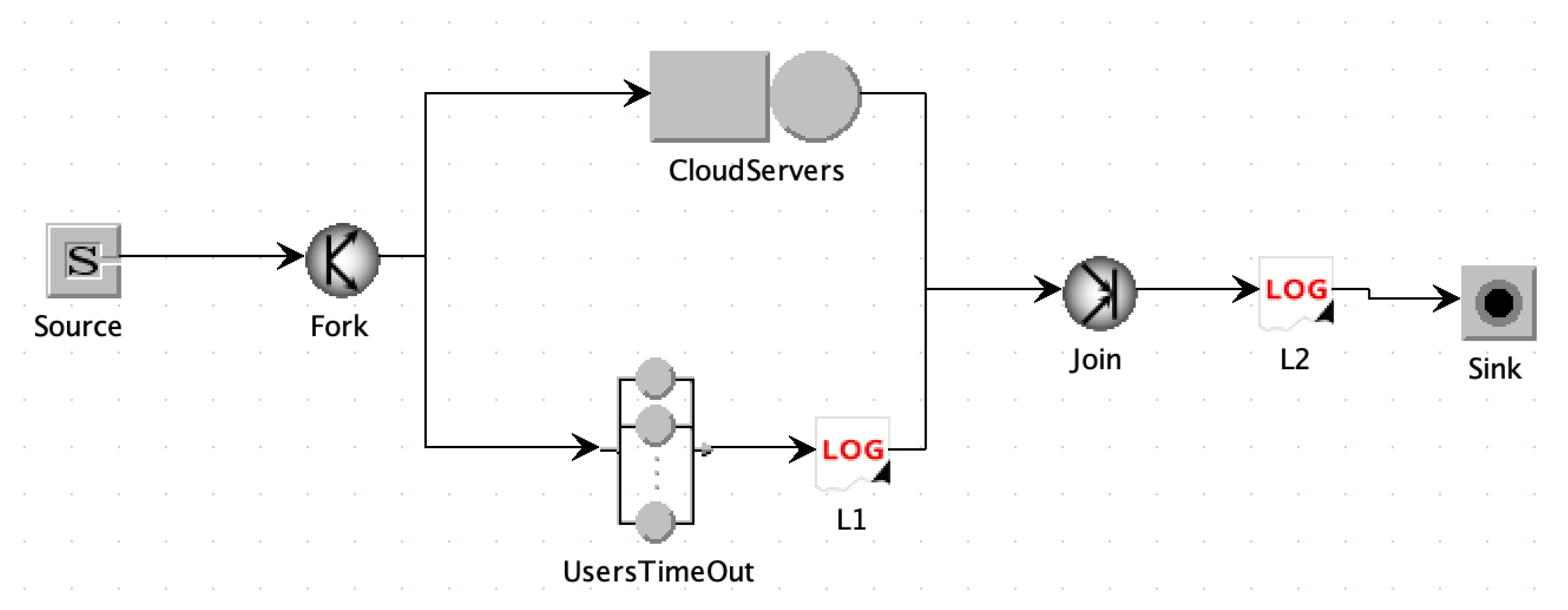
The queuing network depicted in Figure 2 models the application of Figure 1. It is composed of a fork/join that splits a request into two tasks: one models the real request execution (upper branch) and the other represents the occurrence of timeout due to user abandonment (lower branch). The execution of the service demand is modeled by K servers queuing node, while the timeout is modeled by a delay node. The join node waits until the first task is executed (in this case, the quorum is equal to one). The probability distribution taken into account to describe the service demand is hyper-exponential with an average duration of 1 s and a coefficient variation of 5. The timeout is considered to be deterministic, and arrivals are assumed to be generated according a Poisson process: both the duration of the former and the rate of the latter are varied during the study of the model. The two loggers L 1 and L 2 in Figure 2 track the instant of time the request in execution flows through them and allow to compute the probability P ( T i m e o u t ) that a request ended due to timeout. In particular, since the join has zero duration, a request that ends due to timeout will have the same timestamps recorded by both the loggers.

3.1.4. Model results

We start considering requests arriving at rate λ = 1.8 r/s, and a timeout T = 10 s. It is interesting to compare the behavior denoted on the right of Figure 3, where the spikes generated by the services are not depending on a timeout variable and the scenario shown on the left, where the timeout is cutting the service times of the requests exceeding it.
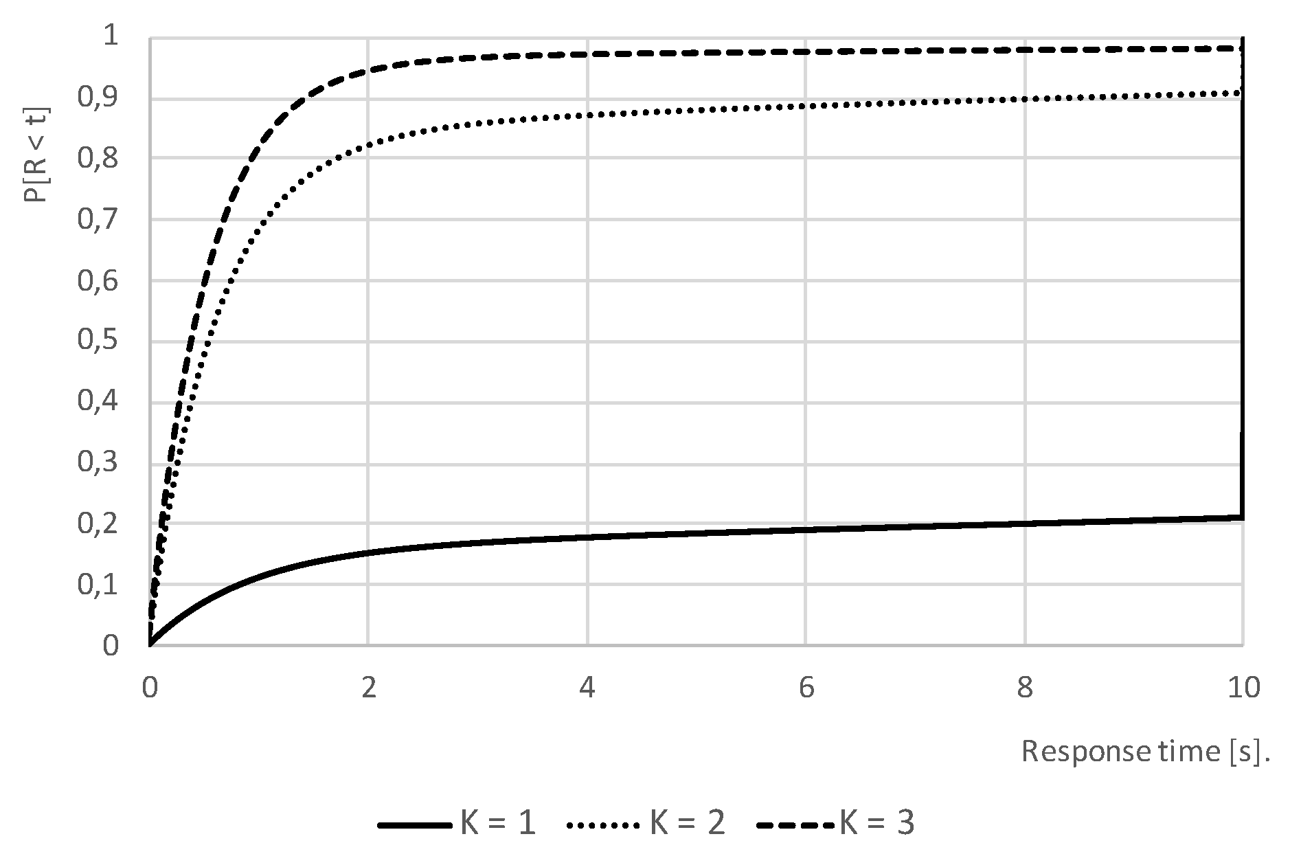
This effect is further investigated in Figure 4, where the response time distribution for different number K of VMs, ranging from 1 to 3, and an arrival rate of λ = 0.9 r/s is presented. Although for K = 1 the system is stable and characterized by an average utilization U = 0.9 , most of the requests will undergo a timeout (the steep rises at time t = 10 s): users are then either served very quickly or quit the system otherwise. With K = 3 , timeout almost never occurs, while K = 2 seems to be a reasonable tradeoff between deployment cost and user experience, where most of the requests are served on time, and only less than 10 % are subject to timeouts.
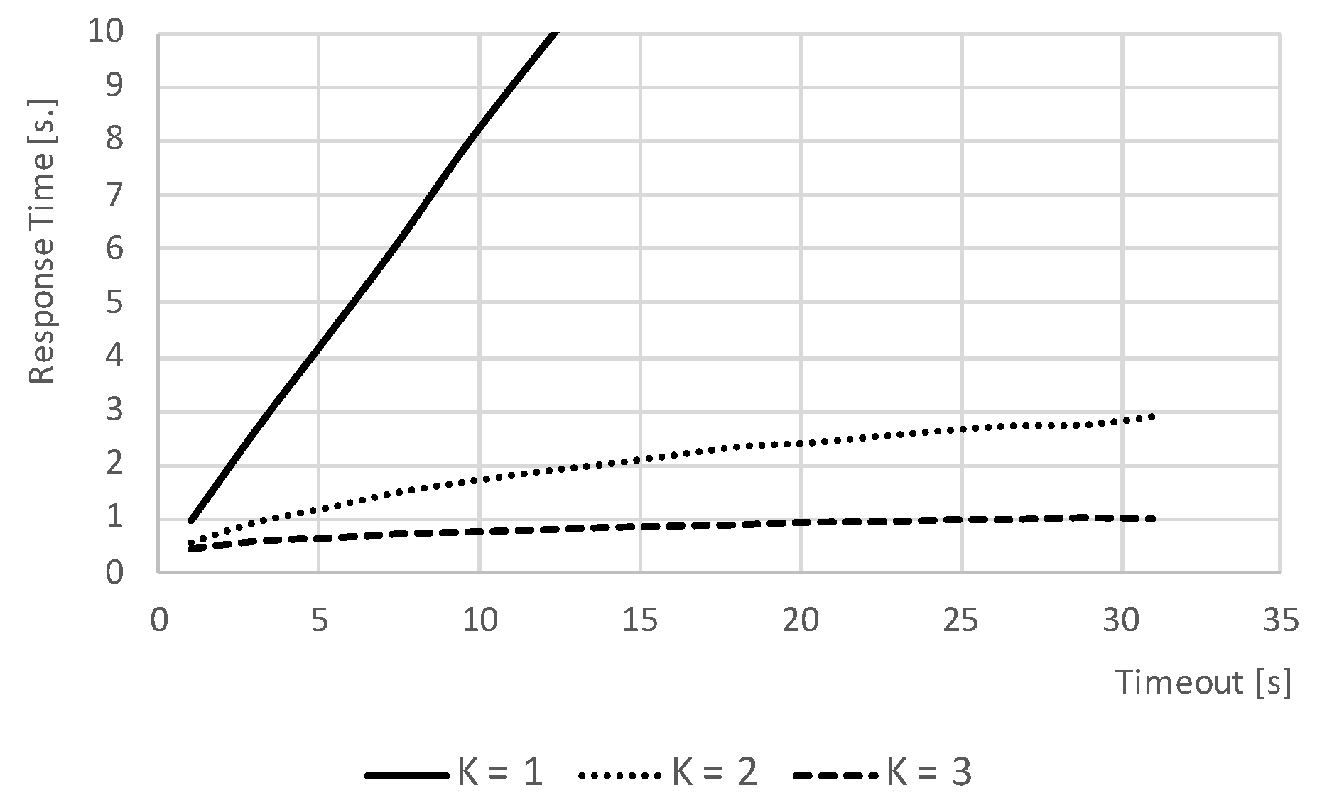
The effect of the deployment on a different number of VMs is then investigated in Figure 5, for increasing timeout durations. With only one VM ( K = 1 ), the users are almost always subject to timeouts, and its value basically defines the time requests will take before being discarded due to abandonment. Parallel deployments ( K = 2 and K = 3 ) are instead only marginally influenced by timeouts, since, in any case, most of the users will be served before the event occurs.
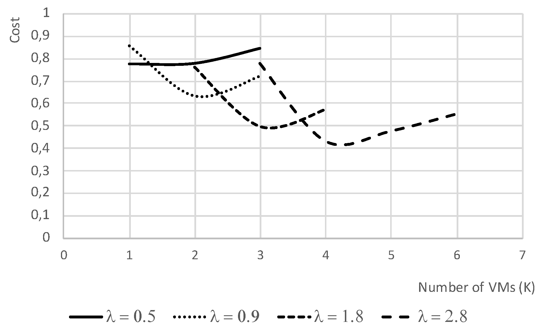
Finally, Figure 6 studies the trade-off user satisfaction and deployment cost, by defining a metric: c o s t = 1 U + P ( T i m e o u t ) where U is the average utilization of the VMs and P ( T i m e o u t ) is the probability that a timeout event occurs, as identified by the two loggers. When the system is deployed on a small number of VMs, the utilization is very high (hence, 1 U is close to zero), but also the timeout probability is close to P ( T i m e o u t ) 1 . Conversely, when the system is deployed on a large number K of VMs, the time probability is close to P ( T i m e o u t ) 0 , but also the utilization is very low, making 1 U 1 . The best configuration of the system is thus the one that minimizes this cost. For an arrival rate of λ = 0.9 r/s, this occurs at K = 2 , while, for λ = 1.8 r/s and λ = 2.8 r/s, at K = 3 and K = 4 , respectively. Note that, in these cases, respectively, K = 1 and K = 2 could not have been used since in such circumstances the system would have not been stable. For λ = 0.5 r/s, the best solution seems to be K = 1 , since having a second VM does not sufficiently decrease the timeout probability.

3.2. Approximate Computing with Finite Capacity Region

The evolution of hardware and software architectures is making approximate computing an emerging technology with great potential. This computing paradigm is based on a very simple concept: an approximate result obtained in a short amount of time is very often sufficient to achieve the objectives of the application with the required accuracy. Essentially, this method trades off accuracy of results with the requested time for their computation.
Examples of applications range from parallel search engines to data analytics, video streaming compression, statistical analysis of large datasets, MapReduce transactions, and special hardware implemented for this purpose, e.g., Neural Network Accelerators. The wide range of applications requires the implementation of many approximation techniques. Among them, the one based on the parallel execution of several tasks of an application and a stopping condition based on the accuracy level required is very popular. Deploying approximate computing in a cloud computing scenario is particularly relevant, as this approach allows containing the costs of autoscaling algorithms by imposing a threshold to the acquired VM numbers (without affecting the performance and maintaining the system responsiveness to the requests’ bursts). The VMs parallelism degree is not increased, at the cost of lowering down the results quality.
In the following, we show a simple model of approximate computing based on parallel computations, implemented with a Fork primitive, and a control condition based on the accuracy level required, implemented with a Join primitive and advanced synchronization [29].
Thus, approximate computing has the potential to benefit a wide range of application frameworks, e.g., data analytics, scientific computing, multimedia and signal processing, machine learning and MapReduce.

3.2.1. Description of the Problem

A car navigation system designed to meet the needs of the users of a smart city must be adaptive to the highly variable conditions set by traffic, municipality constraints, and other unexpected events. Typically, a pipeline of various stages is used. The first one is the alternative route planning that consists of the identification of k alternative paths from source to destination. This step is referred to as the K-shortest paths with limited overlap [30] problem, since the alternative paths should overlap less than a given threshold. The shortest path in terms of distance or average traveling time might not be the optimal one, as several other parameters may have a significant influence on the computation of the best solution. Examples of conditions that must be considered are: (i) traffic status; (ii) layout of the road map; (iii) municipality constraints; (iv) transient work in progress; (v) car accidents; (vi) severe climate conditions; an (vii) other unexpected events. Consequently, the computation times required by the algorithms are highly variable not only because of the different numerical algorithms implemented but also for those other variables considered.
To be effective, the mean response time R (i.e., the time spent by a request in execution in the fork/join region plus the time spent at the Fork waiting to enter the region) of this step for the computation of the best route must be 3 s. To achieve this performance goal, sub-optimal solutions are computed considering only the results of the first k algorithms of N that completed their executions. The model is used to investigate the impact on the best route computation time of the variability of the execution times of the N algorithms and of the subset size k.

3.2.2. Finite Capacity Regions

In this case, queueing network models contain nodes that include, in turn, regions applying specific policies (finite capacity constraints (FCC)). A policy denotes upper bounds on the number of requests that can reside in its service nodes at the same time. Ready customers (contraposed to customers who are waiting at terminals) wait to enter into a FCC and, once they are inside, compete to acquire the available resources. An interesting case occurs when the population belongs to multiple classes. In this case, the constraints undertaken are the following: (i) one bounding the number of customers in a region for a specific class; and (ii) a shared one limiting the number of customers without class distinctions. FCC allows capturing the occurrence of performance saturation effects determined, for example, by memory constraints.

3.2.3. Model Description

The layout of the model is shown in Figure 7. It consists of a fork/join region with a capacity limited of one request. Each arriving request is split at the Fork into six tasks that are executed in parallel. Each task represent a different algorithm for the route computation and is executed by a dedicated processor represented by a Delay node.
In this specific case, it is assumed that the storage does not origin a bottleneck, since all the nodes exploit a local content and their execution follow a fairness policy.
The parameters of the service demands of the six algorithms are reported in Table 2. Their mean values are highly variable (from 1 to 5 s) and their coefficients of variation vary from 0.5 to 5.
The data in Table 2 are assumed to consider a good variety of computation times. For the sake of simplicity, and without affecting the accuracy of the model, we limit the capacity of the fork/join region to one request, i.e., only the tasks generated by one request can be executed in the region. Requests that arrive when another one is in execution wait at Fork node. A typical characteristic of car navigation systems is the presence of fluctuations in the arrival flow of requests. The arrival rate considered in the study is λ = 2 r e q / s with the exponential distribution of the inter-arrival times.
The request exits the fork/join region when at least k algorithms have completed their executions. The Join implements a synchronization rule referred to as Quorum k.

3.2.4. Model Results

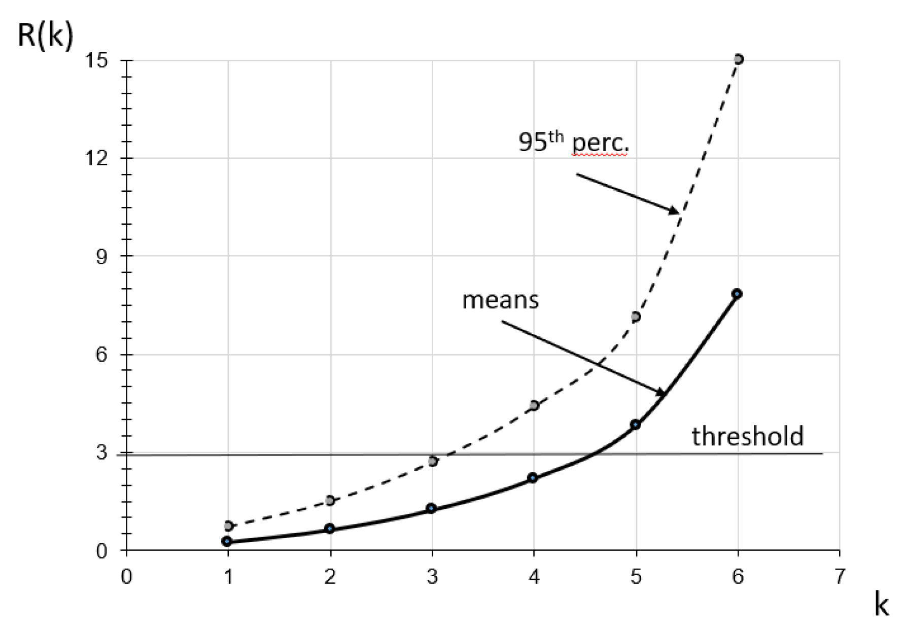
Figure 8 shows the behavior of the mean response times and of the 95th percentiles for the computation of the best routes with respect to the number of algorithms considered from k = 1 ÷ 6 .
The mean values were obtained with 99% confidence intervals.
As can be seen in the figure, it is sufficient to decrease the number k of algorithms waiting for synchronization at the Join from six to five to obtain a 51% reduction in the mean response time (from 7.81 to 3.82 s) and of 52% of the 95th percentile (from 15 to 7.15 s). With k = 4 the mean response time is 2.19 s and the 95th percentile is 4.41 s This value meets the 3 s threshold. The accuracy of the results provided was positively assessed by the data collected in various periods of the day with representative traffic requests.

3.3. MapReduce with Class Switch

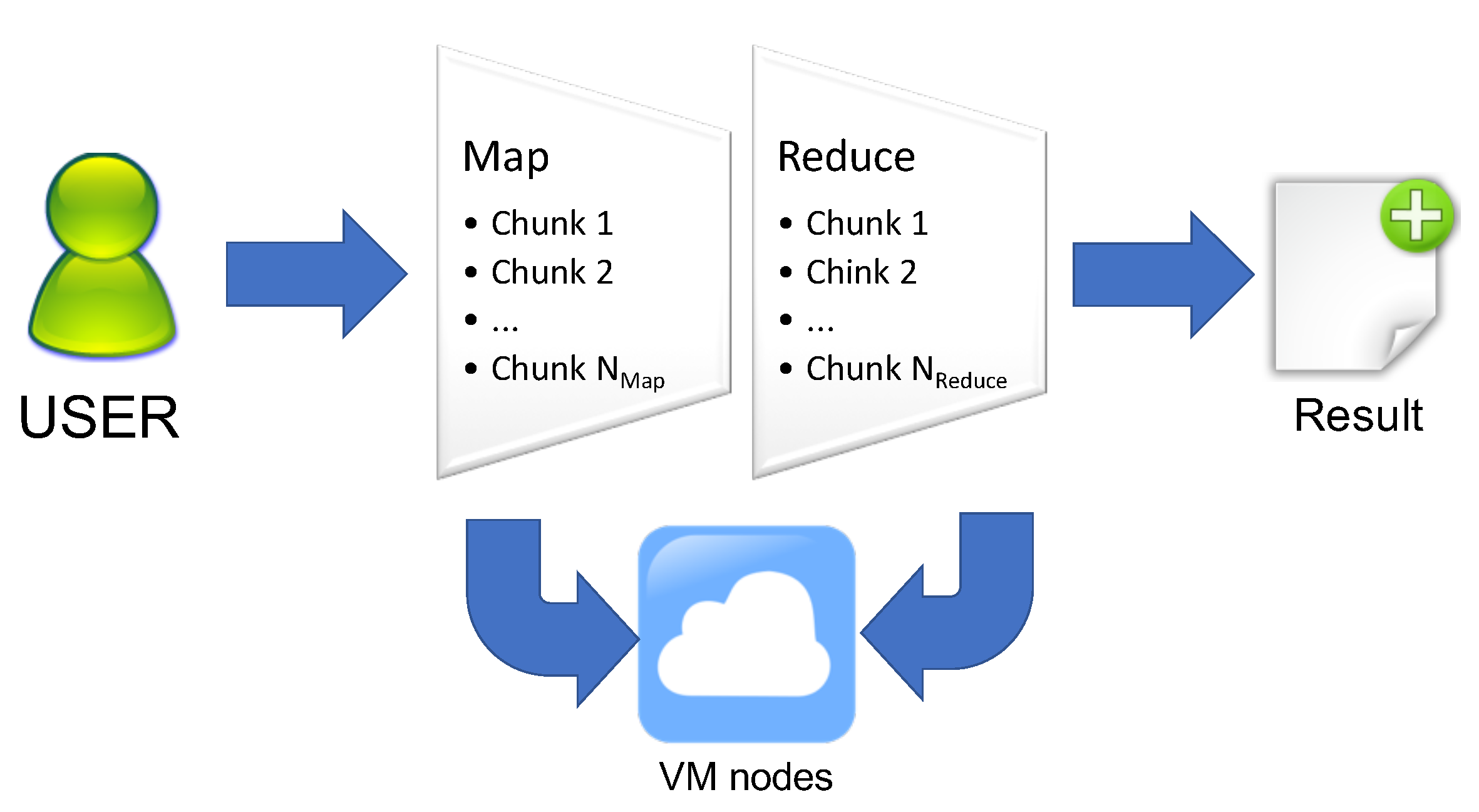
MapReduce is one of the first techniques used to support Big Data applications. From the original proposal by Apache foundation, which was supported by the Hadoop project, several different extensions have been proposed. All the techniques however are based on very similar principles. In short (see Figure 9), all the data that need to be processed (which might consist of Exabytes of data) are split into chunks that are distributed over a large set of participating nodes. Each node, besides storing part of the data, can also perform operations on them. Using specific software patterns, complex operations can be performed to obtain insight information from the considered Big Data collection. MapReduce is the simplest of these patterns: first, the map operation applies a function to each entry of the database, generally performing searching and sorting tasks. The reduce phase collects the intermediate results to produce the final answer. The number of chunks does not necessarily needs to correspond to the number of nodes: in many best practices, the number of chunks is much higher than the number of nodes to increase the parallelism, so that faster nodes can start working on new chunks while the slower ones are still finishing their job. MapReduce is closely related to Cloud computing, since VMs represent the most natural way of acquiring nodes to support the parallel execution process.

3.3.1. Description of the Problem

Sizing a MapReduce application is a non-trivial task. Indeed, increasing the number of nodes decreases the running time of the application. However, due to the hyperbolic decrease and the increasing synchronization complexity, after a given point (depending on the application and on its demands), performance improvements become negligible at first, up to another point, where increasing the nodes only makes the system’s behavior worse. Performance modeld are thus of paramount importance to correctly decide the optimal number of resources, to obtain the best results with the least expense.
While fork/join paradigms are the basis for modeling MapReduce such as in big data processing environments, they cannot capture the fact that the same processing nodes are used in different ways for different stages of the algorithm (i.e., map and reduce). The class switch feature, introduced in the next section, becomes the key tool to model such behavior.

3.3.2. Class Switch

One of the main assumptions adopted when working with simple QNs concerns the type of customers, who are assumed identical from a statistical point of view. However, when regarding a real system, this assumption does not necessarily hold as more parameters, such as the service time and the routing probabilities, must be taken in account. Therefore, it is necessary to postulate the existence of different types of customers by introducing the terms of chain and class. The former identifies a situation where a customer belongs to the same type during the entire execution. The latter denotes instead a temporary classification: from this perspective, a customer is able to change from a class to a different one while executing within the system according to a probability. The type of class plays an important role in characterizing the customer service time (in each node) and the routing probability. Classes can be partitioned into chains, which prevents the case where a job switches from classes that are part of different chains. A class switch operation allows a customer in chain to change its appearance to the server, by presenting itself with another class.

3.3.3. Model Description

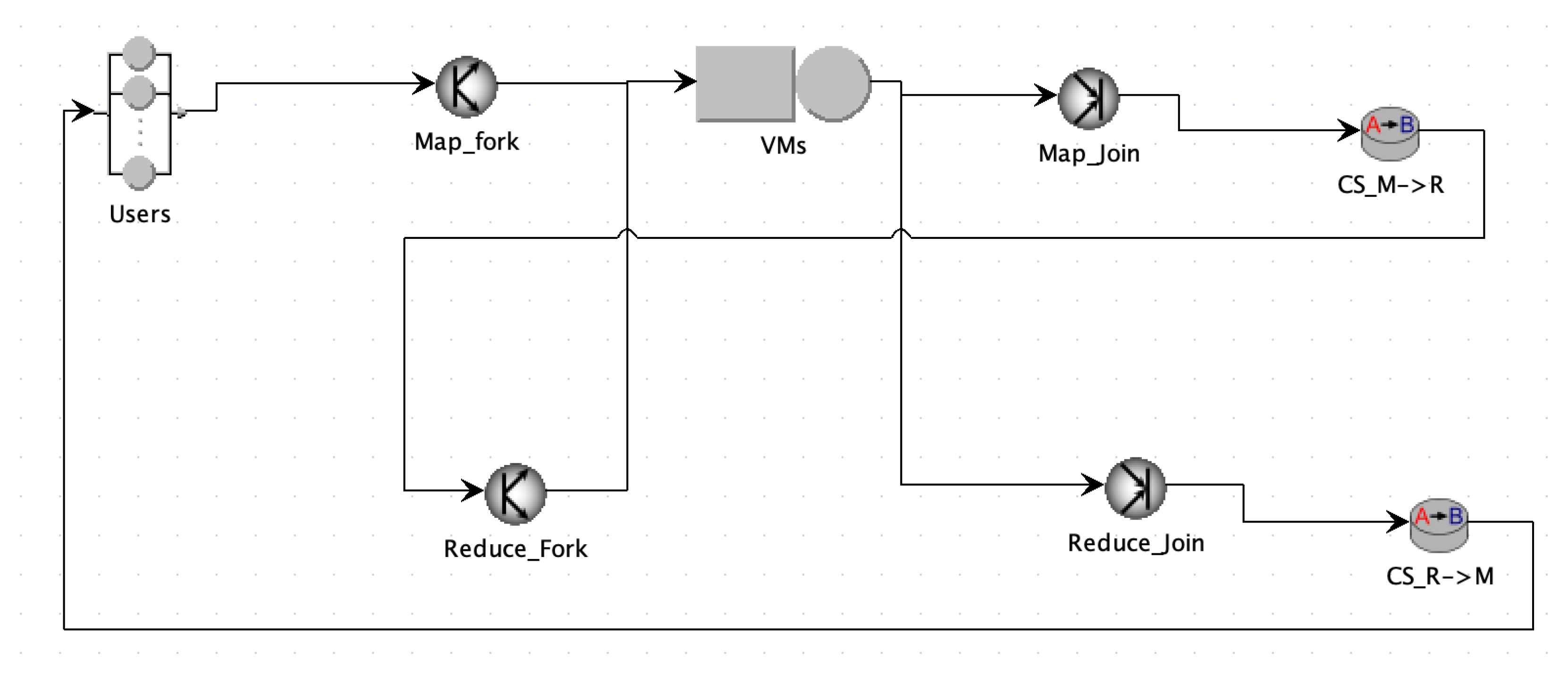
A simple MapReduce application is presented in Figure 10. In particular, we consider N users who, every Z = 100 s (modeled by delay node U s e r s ), submit a map–reduce job to the system. There are two classes in the system, representing, respectively, the map and reduce stages of the application. All requests starts in the map phase, and are characterized by the corresponding class. The Map_fork node splits the job into M_Map tasks, which are then rejoined in node Map_join. The class switch node CS_M->R changes the class of the job to the reduce stage, which is immediately split into M_Red reduce tasks in node Reduce_Fork. The job is finished when all the reduce tasks terminate: this is modeled by the join operation performed by node Reduce_join, immediately followed by class switch node CS_R->M that restores requests to the starting map class. All tasks are served by the K server queueing node VMs modeling the cloud environment running the application. The service time of the all the VMs is assumed to be exponential, with a different duration D_Map and D_Red, respectively, for the map and reduce stages. In the next experiments, we assume M_Map = 64, M_Red = 32, D_Map = 1 s, and D_Red = 2 s.

3.3.4. Model Results

The system is studied for a different number of users N, starting with N = 10 and up to N = 50 , for different parallelization levels K (corresponding to the number of acquired VMs).
Figure 11 shows the average number of tasks in execution in the VMs for the map and the reduce stage. As expected, it grows with the number of users N, and decrease with the number of K VMs. It is interesting however to note how the decay is not linear, but not even clearly hyperbolic: this is due to the different configurations of the map and reduce stages.
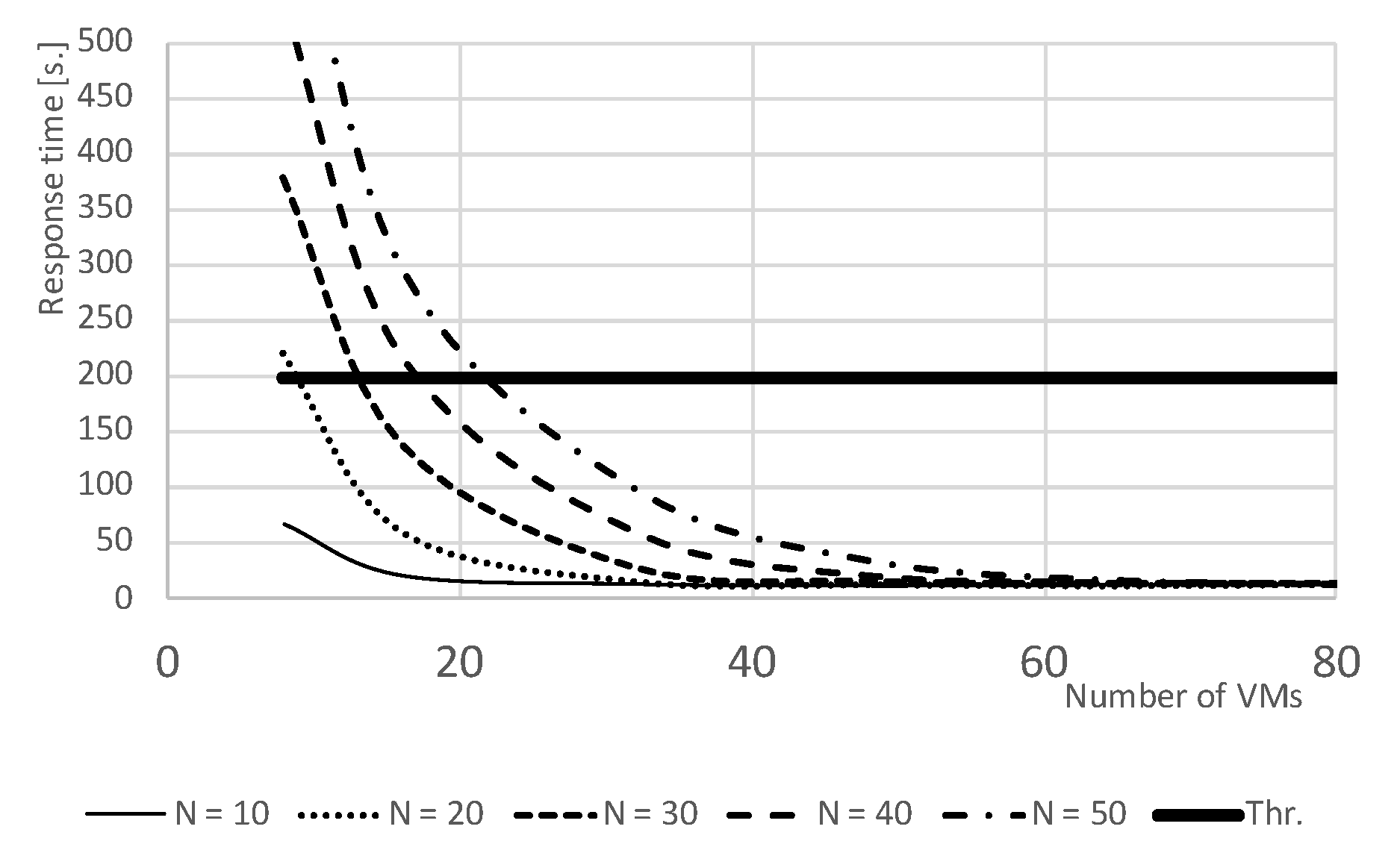
Figure 12 shows an exploitation of the model to determine the best number of VMs to support a given number of users N. In particular, it explains how the model can be used to size the system to achieve a target average response time τ = 200 s. When the number of users is very low ( N = 10 ), even a small number of VMs ( K = 8 ) is able to provide average response time much lower than the threshold. However, with a population of N = 50 , at least K = 24 VMs are necessary to achieve acceptable performances. It is also interesting to see that, for K 64 , all the considered configurations have basically the same lowest performances: this is because each job is split into M_Map = 64 tasks. If no other job is currently running, with K 64 all tasks can be executed in parallel in one shot.

4. Multi-Formalism QN/PN Techniques

According to multi-formalism, different part of a system can be modeled by using different formalism flavors (the choice depends on the modeler’s familiarity with one or more languages). In this way, it is possible to lower the learning curve and match the user abstraction as a result. The model thus derived can be solved by defining the proper combination of formalisms by mapping the model concepts into solvers primitives. Multi-formalism has proven to be successful in different areas such as biology, fault-tolerant computing, and disaster recovery. As a result, this interdisciplinary aspect has created interesting links between different communities of modelers. Various different software tools have been implemented to date. With regard to JMT, the considered multi-formalism approach allows the integration of queueing networks (QN) and Generalized Stochastic Petri Nets (GSPN, see [31] for the theoretical background of this formalism).

4.1. Hybrid Cloud

A hybrid cloud consists of an on-premises infrastructure, based on a private cloud, and resources acquired as-a-service from a public cloud provider. Among the various factors motivating a boost in the diffusion of these architectures are high security, controlled performance, large scalability, fast adoption of new technologies, and cost savings.
The problem of scalability in hybrid clouds is typically addressed through the dynamic provisioning of resources from the public cloud. The model presented in the following case study addresses this problem by implementing an algorithm that dynamically routes the requests to the public cloud when the load on the private component exceeds a threshold value.

4.1.1. Description of the Problem

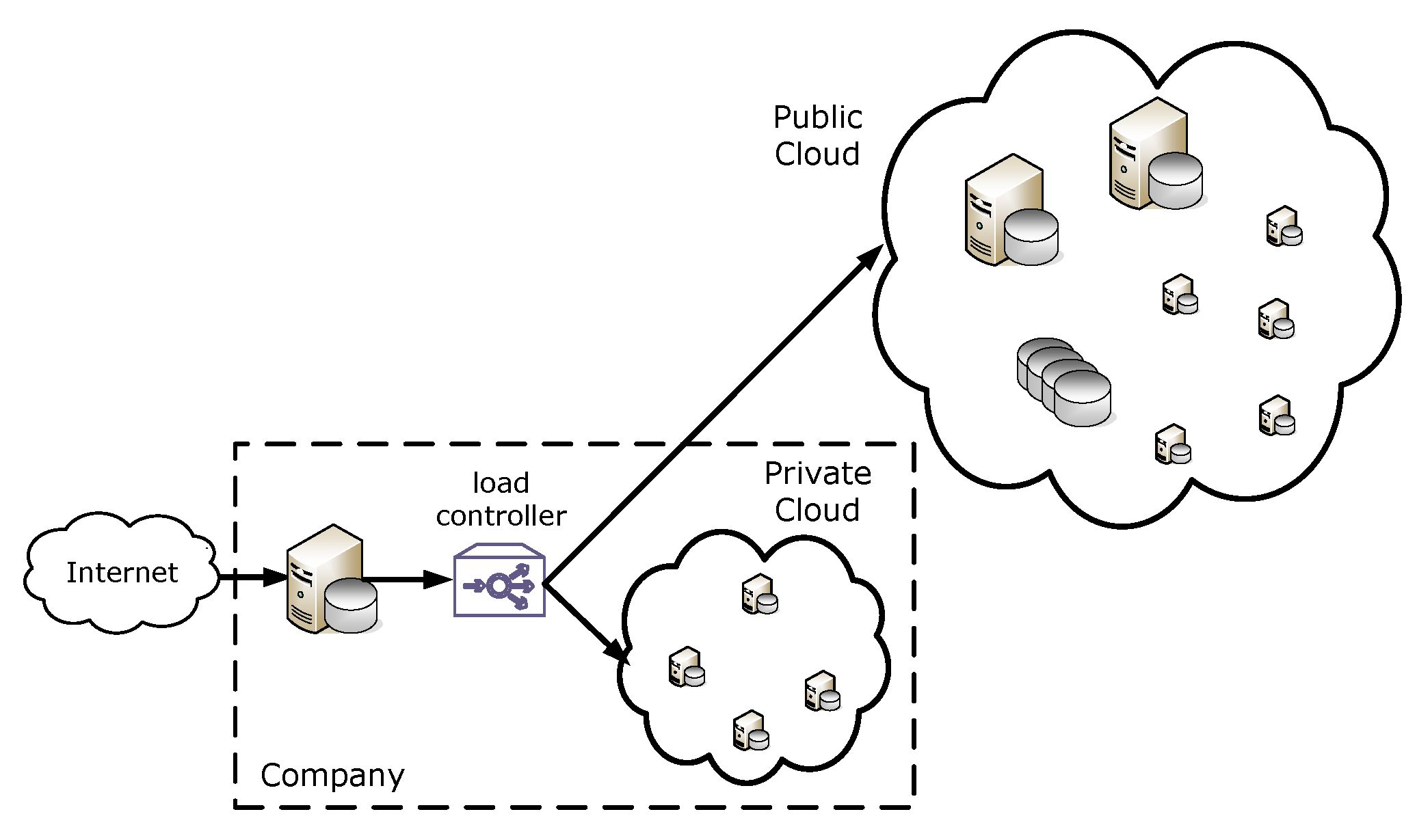
This case study concerns a model of an IT infrastructure based on a hybrid cloud. More precisely, it focuses on modeling the process for dynamic resource provisioning. This method is able to acquire VMs on-demand from the public cloud when requests exceed the capacity set as a threshold on the private cloud. The multi-formalism model implemented consists of elements of Petri nets and queueing networks. The hybrid cloud scenario considered is represented in Figure 13.
The incoming requests are processed by the user interface of the application and, after some formal and security checks, are sent to the load controller module. To satisfy the performance requirements, the software architecture of the app has been designed assuming that a dedicated VM of the local cloud is assigned to each request in execution. Since several highly fluctuating workloads share the resources of the private cloud, a limit is set on the maximum number of VMs dedicated to this application. When this threshold is reached, the new VMs are acquired on-demand from a public cloud.
The impact of this threshold on global response time and throughputs of both clouds need to be investigated. The objective of the study is the identification of the computational capacity, in terms of number of cores and power, of the servers of the private cloud that are required to satisfy the performance target with cost savings. In fact, VMs with the same computational power as a private provided by the public cloud are much more expensive. Therefore, to save costs, the VMs provided by the public cloud are much less powerful than the private ones. Thus, there is a tradeoff between the VMs provided by the private and public clouds, of performance and infrastructure costs.

4.1.2. Model Description

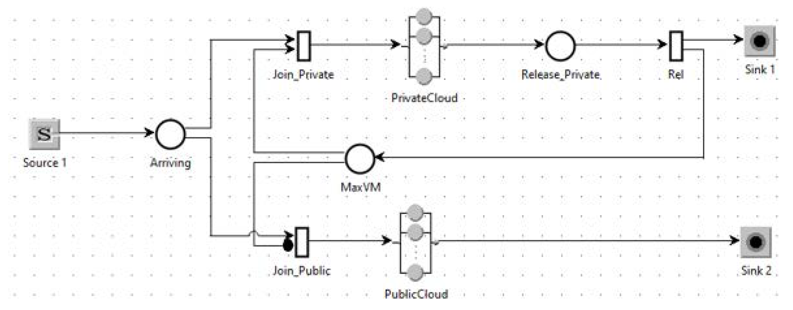
The layout of the model is shown in Figure 14. The workload consists of two classes of customers: the incoming requests, representing the user demands of computation time, and the VMs (the tokens), representing the number of VMs available in the private cloud.
The JoinPrivate transition is enabled when a request arrives in Arriving place and there is at least one token available in MaxVM place. Each time the transition is activated, a VM of the private cloud is assigned to the request and the value of MaxVM is decreased by one. When this value is zero, the Inhibitor arc from MaxVM place and JoinPublic transition activate the latter and the request is addressed to the public cloud. When a request has been completely executed in the private cloud, the Rel transition routes it to Sink1 and a token is sent to the MaxVM place incrementing the number of VMs available.
The two clouds are represented by two delay stations since there is no competition for an available VM in both clouds. The arrival rate of the requests to be considered in the study is λ = 50 r e q / s . This value has been assigned by the application designers since it is representative of a medium/high load that, according to the business plan, should be achieved in a year. The fluctuations of arrivals has been modeled with a c v = 4 of the hyper-exponential distribution of inter-arrival times. The mean service demands of the private cloud is 2.5 s while those of the public cloud is 7.5 s. The high variability of service times was considered assuming their distributions as hyper-exponential with c v = 6 . The time required by the processing of a request in the other infrastructure components, such as the user interface and the load controller, are negligible compared to the service demands of the VMs; therefore, small increases in their values have been considered.

4.1.3. Model Results

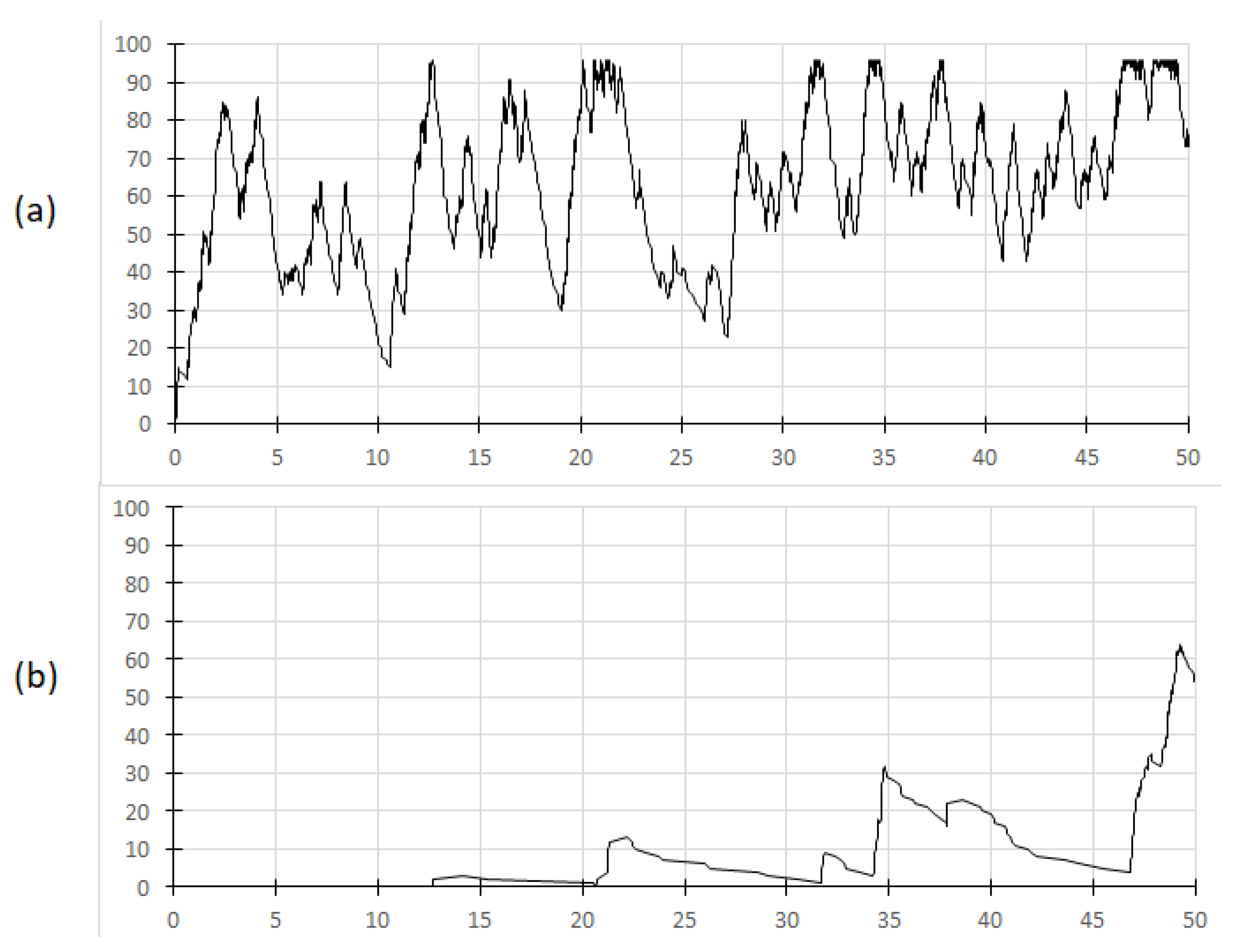
The behavior of the algorithm for dynamic provisioning of virtual machines is highlighted in Figure 15 that shows the trend of the number of VMs in execution in the two clouds, private (Figure 15a) and public (Figure 15b), in the interval 0–50 s.
The arrival rate is λ = 50 req/s and the threshold of the VMs in the private cloud is 96. As can be seen in Figure 15a, when the number of requests in execution in the private cloud is greater than 96, the provisioning of the new VMs is dynamically routed to the public cloud (see, e.g., the interval 45–50 s in Figure 15b).
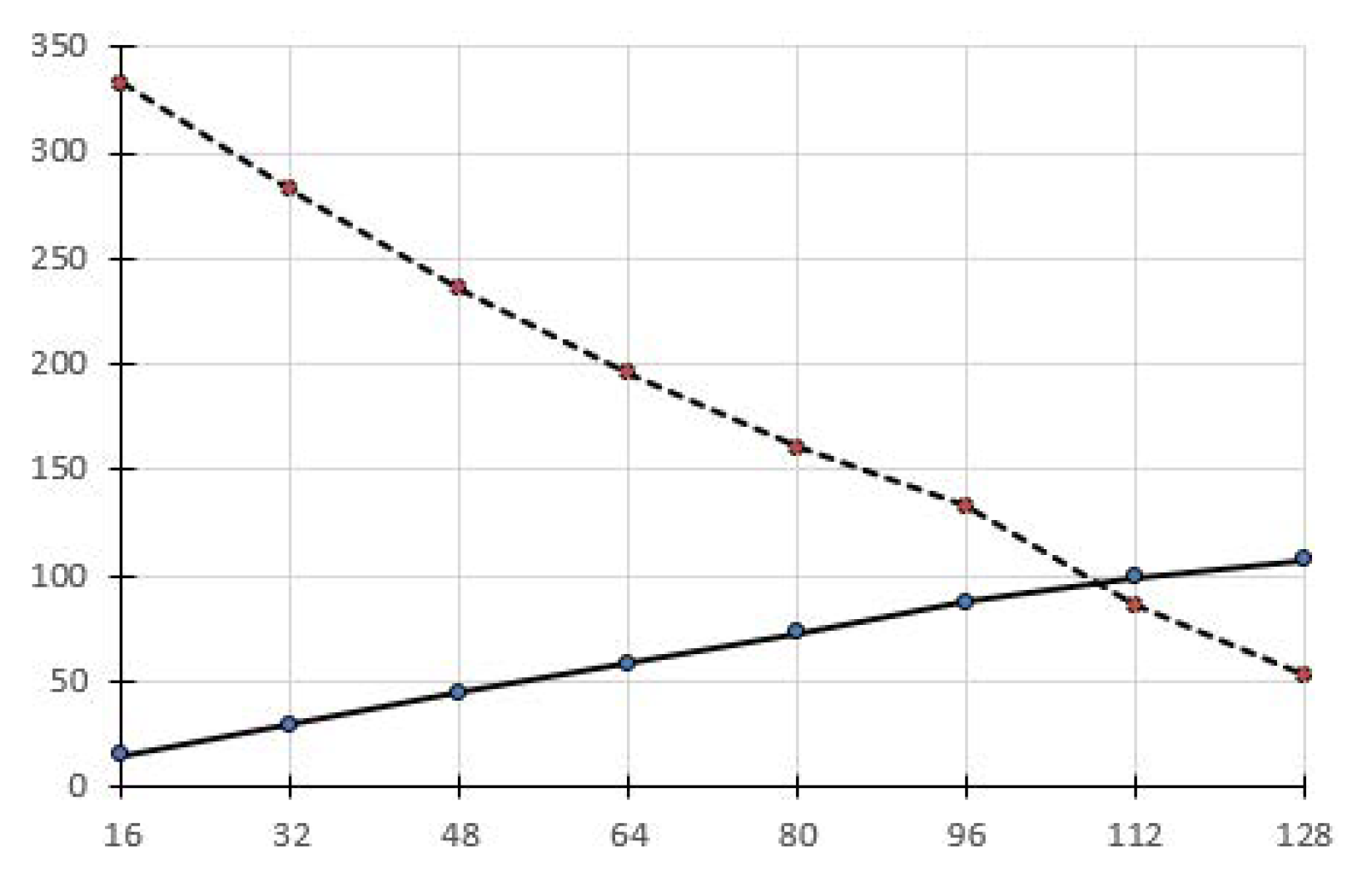
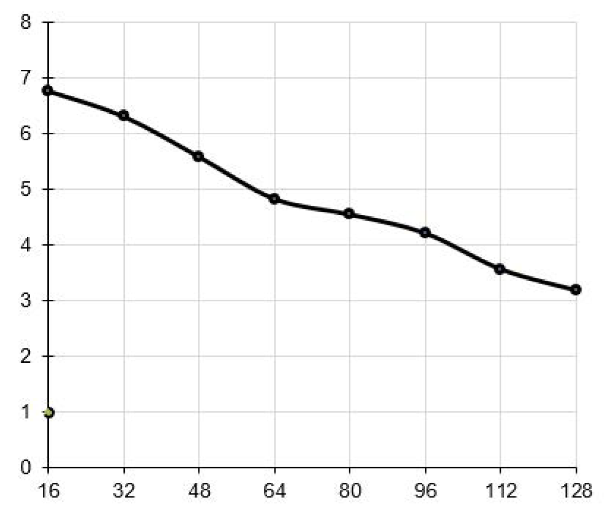
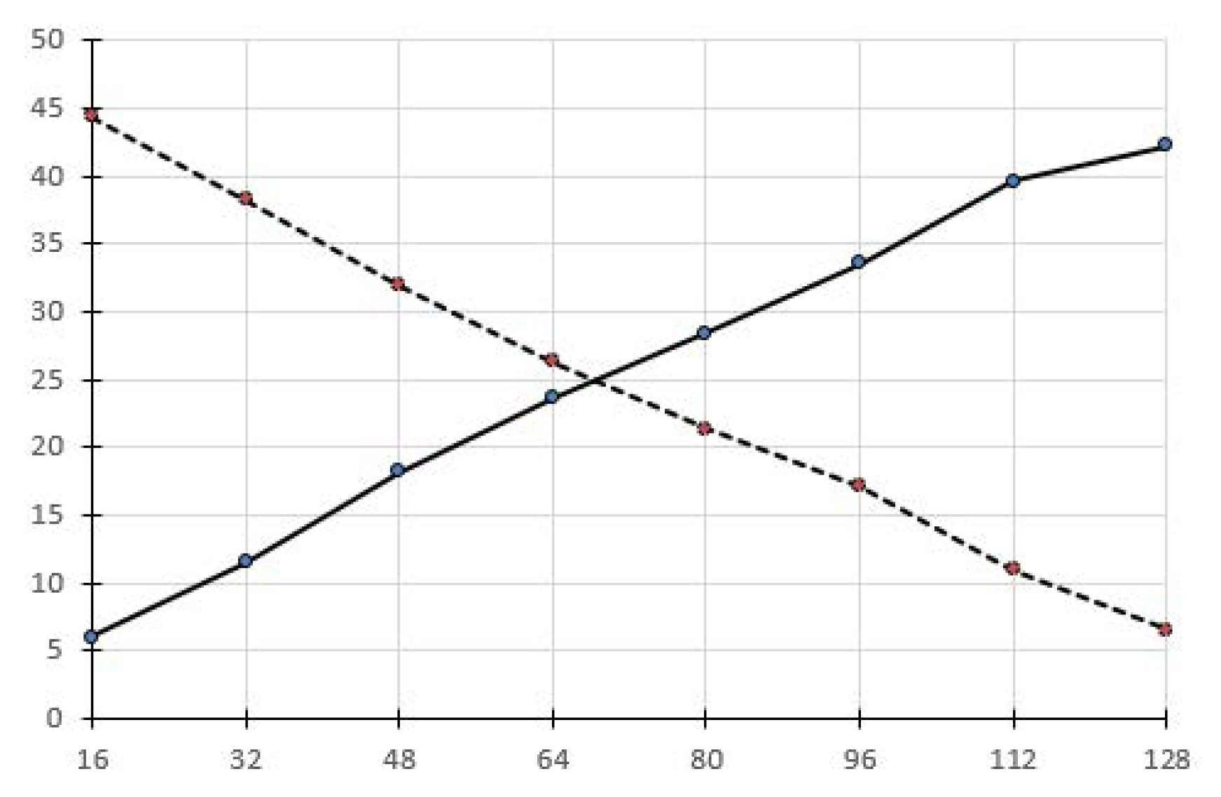
The number of requests in execution in the two clouds as a function of the maximum number of VMs MaxVM that can be provisioned in the private cloud is shown in Figure 16. The range of MaxVM evaluated is 16–128. The mean response time R of the system as a function of the MaxVM is depicted in Figure 17.
With 96 VMs, the average response time is close to 4 s, a value that is considered acceptable as a performance target with the associated costs. As can be seen in Figure 16, 87 VMs are in execution in the private cloud and 133 in the public cloud with MaxVM = 96.
The costs of the infrastructure can be evaluated considering the throughput of the two clouds as a function of MaxVM (see Figure 18).

4.2. Batching in IoT-Based Healthcare

The proliferation of IoT in the healthcare scenario has introduced new problems, which have been faced for effective use of their potential. Important benefits can be obtained in all areas of e-Health, in particular in those that use IoT integrated into information infrastructures enabling the use of ubiquitous computing technologies. Patients can be monitored anytime and anywhere, in either special hospital wards or remotely, through the use of wearable sensors and smart medical devices.
Sensors may detect a variety of patient physiological signals, such as temperature, pulse, oxygen saturation, blood pressure and glucose, ECG, and EEG, as well as other body motion related variables that can help accurately monitoring patient movements. Among the potential benefits that can be achieved by body sensors, and more generally by IoT smart devices, in e-Health monitoring are the high rate of data transmission and the minimization of end-to-end data delivery time. The interconnections among the various components of the networks, e.g., IoT devices, intelligent medical devices, edge and fog systems, hospital and cloud servers, patients, and medical staff, are implemented through cabled or wireless networks with low-power communication protocols.
The following case study focuses on body sensor networks, and more specifically on the study of the trade-off that exists between performance of the network (data delivery time) and the energy consumed by the data exchange (the cost of transmission).
The implemented model is derived from a more complex version of the one in [32] that considers a completely different scenario: the smart monitoring of fog computing infrastructures. The key feature of these models is the dynamic management of the buffer of requests based on the intensity of arrivals and the expiration of a periodic trigger. With the multi-formalism models, it is possible to implement algorithms with dynamic behavior as a function of the workload characteristics.

4.2.1. Description of the Problem

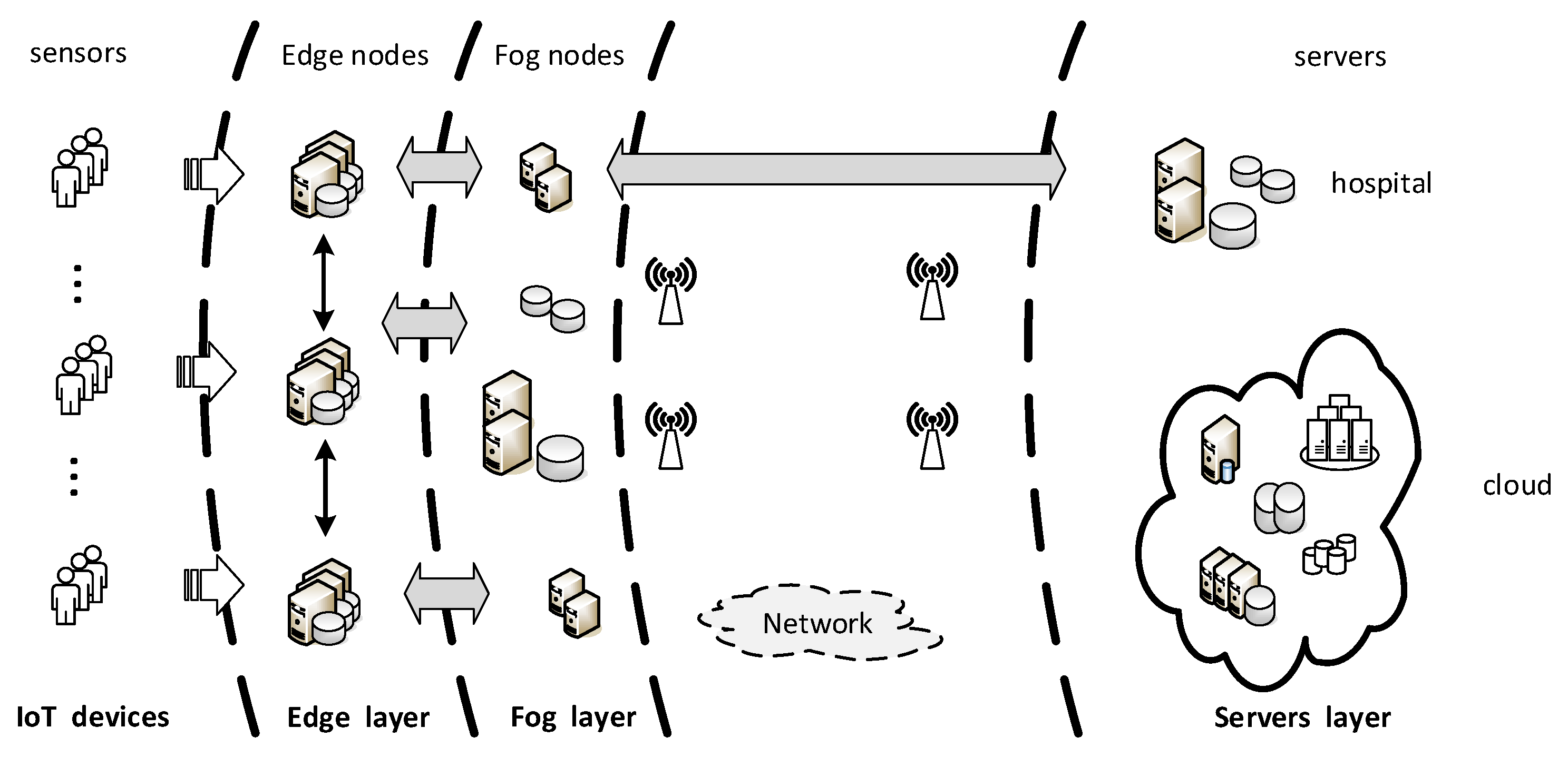
Figure 19 shows the target e-Health scenario considered. The data collected from body sensors are transmitted through wireless or wired connections to the edge nodes located as close as possible, where they are pre-processed and then sent to the fog nodes (if any) or to the hospital servers for their complete processing.
The data arriving at the hospital servers are subject to fluctuations generated by the different type of physiological signals detected and the health conditions of the patients. Indeed, different type of measured variables require a different frequency at which a detected signal is available for transmission. For example, in body temperature, the sampling rate can be once per minute; in pulse oxygen monitoring, the rate can be once per second; and, in other variables, such as ECG or EEG, it can be of the order of several hundred per second. In addition, when a patient’s health condition is assessed as critical, new sensors are activated and the detection rate of other monitored variables can be increased under the control of edge or fog nodes. Among the many problems that need to be addressed, this case study concerns the following:
  • identification of the amount of data that must be considered in each transmission to hospital servers in order to satisfy the performance requirement in term of end-to-end data delivery time and minimize the energy consumption of the operations; and
  • identification of potential critical health conditions of patients that need urgent investigation, i.e., fast response time.
The former problem requires studying the trade-off between the time required to deliver the detected signal to the servers in the upper layer of the medical infrastructure, and the cost associated with the transmission operation. The immediate transmission of a detected signal minimizes its end-to-end response time from either the hospital servers or the cloud. However, the set up costs of the connection cannot be shared with other signals. The technique of batching the data of several signals to be transmitted in a single operation is used to approach this problem. The impact on end-to-end delivery time of different batch sizes, and thus on the number of operations required to transmit the signals detected by a set of sensors, must be studied. Knowing the number of sensors connected to an edge system and the type of signals detected, it is possible to derive the arrival rate of the requests to the hospital servers. Then, once pre-processing is complete, the data are stored in a buffer until they are ready to be transmitted. The management of this buffer is crucial to achieve the two objectives described above.
The implemented algorithm considers the number and types of signals detected by the sensors connected to the edge nodes, the fluctuations of arriving traffic considered regular and the arrival patterns that must be transmitted with p r i o r i t y , as they can be associated with a patient in critical conditions. The most important elements of the implemented model simulating this algorithm are described in the next section.

4.2.2. The Model

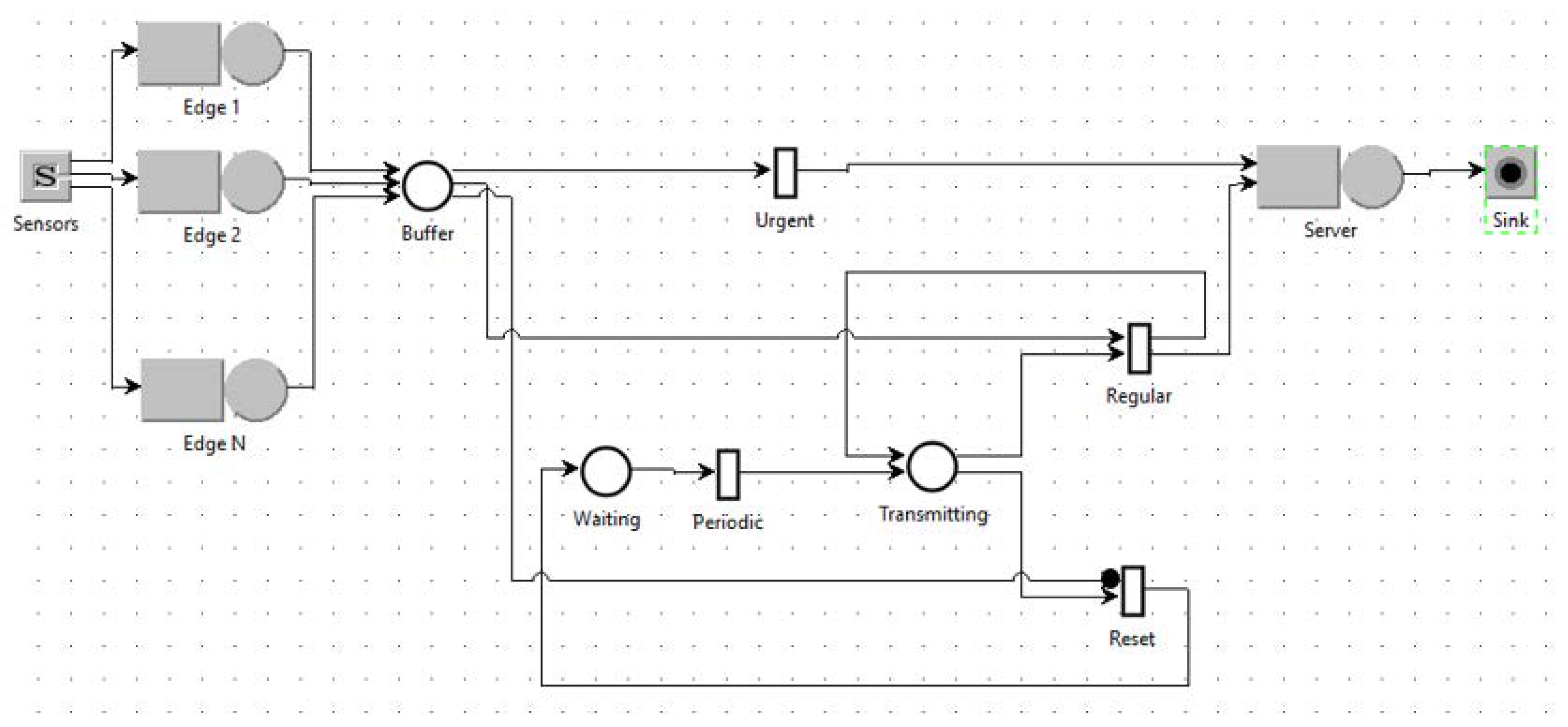
Multi-formalism models allow the exploitation of queueing networks and Petri net primitives to represent each concept with the most appropriate technique. To describe the dynamic behavior of the batching algorithm, we used the PN primitives while the QN primitives were used to represent the other components of the e-Health infrastructure. The layout of the model is shown in Figure 20.
The workload consists of two classes: s i g n a l s detected by sensors (referred to as requests) and a t o k e n , needed to model the periodic/triggered management of the requests.
The key feature of the model is the algorithm that manages the transmission requests batch. To ensure that the model and the presentation of the algorithm remain as simple as possible, we adopted several assumptions that have a minimal impact on the performance but that greatly simplify the description of other parts of the model.
The set of physiological signals detected by each patient is the same, and each edge system monitors several patients. The computational power of the hospital servers has been oversized compared to the processing time required by signals. In the model, we do not explicitly represent the fog systems since their processing time per request is negligible compared to the service time required by the Edge nodes. Moreover, they were considered as small increases in the service times of the Edge nodes.
The global arrival rate λ of data generated by sensors is modeled by all the source Sensors as a single aggregated Poisson process of rate λ . This flow is evenly distributed among the edge systems modeled with Edge queuing nodes. The times required to process the data of a signal, i.e., the service time of a visit by an edge node, are exponentially distributed with mean D E d g e = 200 ms. At the end of this processing phase, the requests are buffered, i.e., routed to the place Buffer, and ready to be transmitted. They are transmitted to the hospital servers (or the cloud servers) that must perform their complete analysis requiring a service time exponentially distributed with mean D s e r v e r = 500 ms. Requests follow two paths: one for Regular requests and one for Urgent requests. The requests in the buffer are managed according to two different policies:
  • The buffer is emptied (i.e., the requests that are in the buffer are transmitted) periodically with a period defined according to the number and type of signals detected by all sensors. Requests are assumed to belong to patients under Regular conditions and are sent at the end of the period.
  • The buffer is emptied when the number of requests in the buffer reaches a threshold value β , i.e., the maximum batch size. In this case, requests with such a high arrival rate are assumed to indicate the presence of a critical condition for one or more patients. Therefore, requests in the buffer are considered Urgent and must be sent immediately without waiting for the end of the emptying period.
The periodic transmission of Regular requests is modeled by the loop between places and transitions Waiting, Periodic, Transmitting, and Reset. The deterministic firing time of transition Periodic represents the duration of the clock for the transmissions of the requests arrived in Buffer. This value is computed by analyzing the detection rate of the sensors in normal operating conditions. According to the configuration analyzed, we considered 15 s as constant firing time of the transition Periodic (i.e., as periodic empty cycle time). As soon as the empty cycle expires, a token is transferred to place Transmitting where two alternatives are possible. If there are requests in the buffer, the immediate transition Regular will be enabled and will transfer them to the transmission channel. When the buffer is empty, either because all requests have been transferred or because no requests arrived in the periodic time frame, the immediate transition Reset fires, due to an Inhibitor arc that connects it to the Buffer, and restarts the timer.
The Urgent requests are managed by the immediate transition Urgent that is connected to place Buffer with an input arc of weight β . When the threshold value β is reached, the batch of requests in the Buffer are immediately transmitted to the hospital server. Note that also the arc that exits the transition Urgent has weight β , since the entire batch of requests is sent to the server.

4.2.3. Model Results

We considered several configurations of the system by modifying the global arrival rate λ , the threshold β of Urgent requests, and the empty buffer cycle time. In this section, we limit the description of the results to those that emphasize the impact of the dynamic management of the buffer of requests on the performance of the system and related costs.
The arrival rates of the requests considered in the study are λ = 0.1 ÷ 1.9 r e q / s . The inter-arrival times are exponentially distributed. These values were assumed to be representative of the potential number of patients in an emergency ward of small- or medium-sized hospitals.
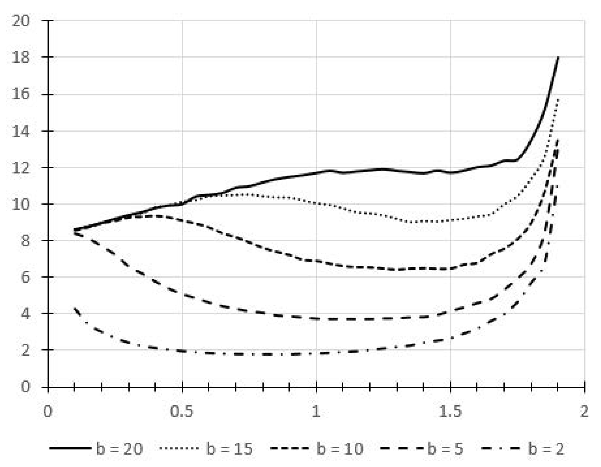
Figure 21 shows the behavior of the System Response Time R, i.e., the end-to-end time required by a signal from its detection to the completion of its processing by the hospital server, for the complete range of arrival rates. The family of curves refers to different values of β , from 2 to 20, i.e., the threshold for the identification of Urgent batches of requests will be transmitted immediately.
With a λ increase, we model an increase in the number of sensors or in the detection rate and the workload managed by Edge nodes is also greater. For small values of β (2 and 5), there is an initial decrease of R. This is because, with such small sizes, nearly all batches are considered Urgent and therefore most requests are transmitted almost immediately when they join the Buffer. With larger values of β (10, 15, and 20) this initial decrease of R as λ increases is not present. When λ becomes greater than 0.1 the value of R starts to increase from the beginning. With these batches sizes, R begins to decrease for larger λ values than those obtained with smaller β . The motivation for this behavior is that, as λ increases, the number of requests in the buffer increases as well, and if β has higher values the threshold is reached with less probability and the number of batches transmitted when the period expire is greater. However, with further increases of λ , the threshold is reached more easily and therefore there is a shorter waiting time for the requests in the buffer, i.e., the Urgent requests increase. When λ is greater than 1.5 req/s, R increases for all β since the response time of the highly utilized hospital server becomes the dominant part of its value.
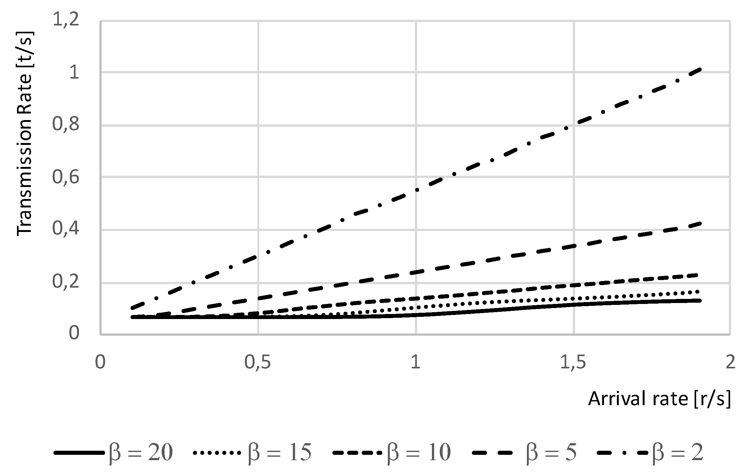
According to the objectives of the study, the R values should be analyzed together with the cost (energy consumption) for transmissions. It is assumed that the cost is directly proportional to the number of times a batch is transmitted, i.e., a buffer is emptied. Indeed, the greater are the number of times and the sizes of the transmitted requests at the same time, the better is the energy efficiency of the system. In Figure 22, the transmissions per second are shown for all the values of the considered λ .
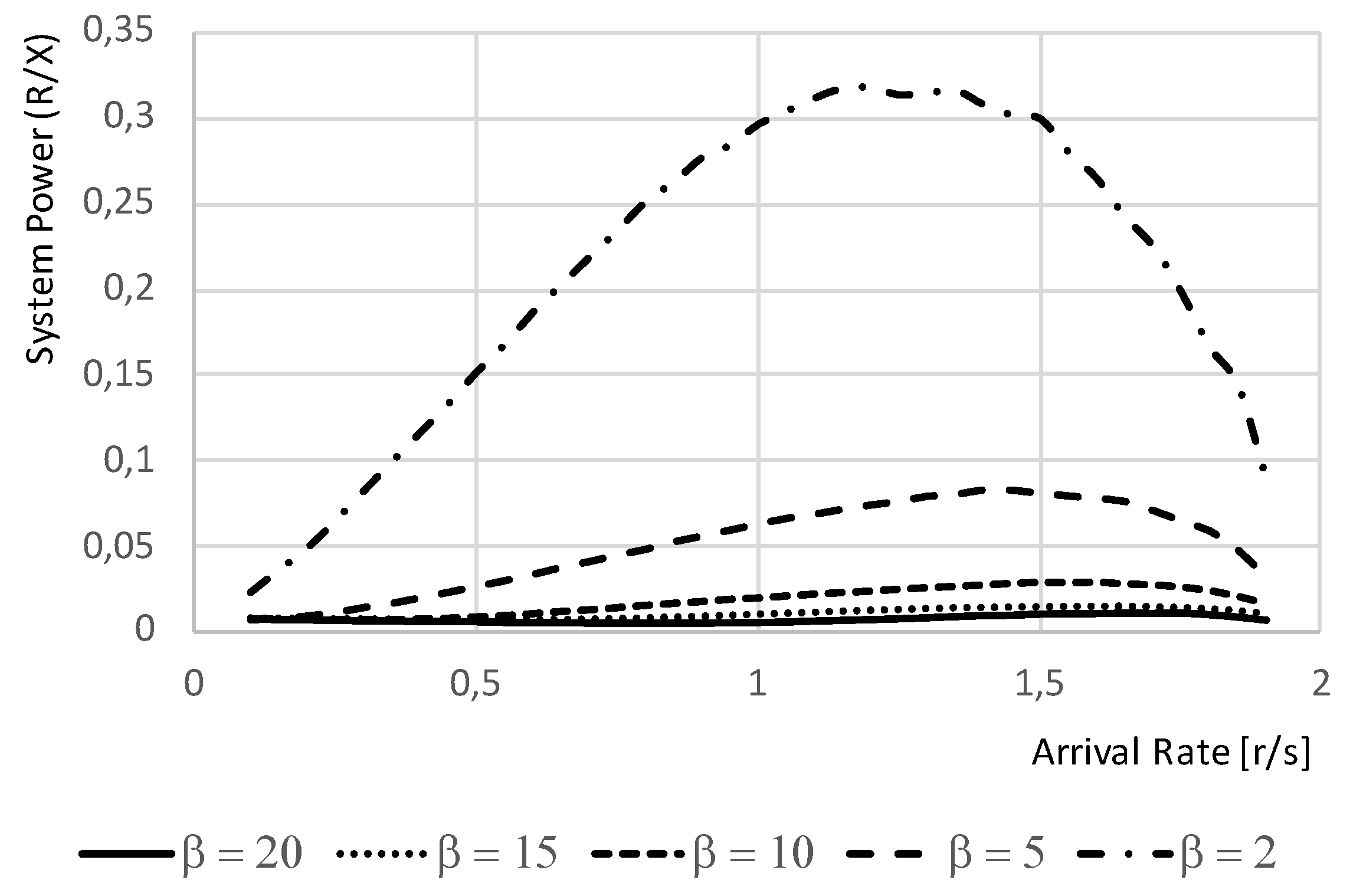
As expected, with batch size β = 2 , the number of transmissions per second are the highest, while the minimum for β = 20 . However, to have a meaningful result, these values should be considered together with the system response times. To this end, the metric system power, introduced in [33] and combining the throughput X of a system with its response time R, is considered. This metric is the ratio X/R of throughput and response time, and captures the level of efficiency in executing a workload. The maximum power corresponds to the optimal operating point for the system, i.e., the point at which the throughput is maximized with the minimum response time. In our system, we have considered the ratio of transmissions/s and aystem response time. Figure 23 shows the ratio of the two metrics of Figure 22 and Figure 21.
The optimal operating points of the system are clearly identified as a function of the batch size β for the Urgent requests and the global arrival rate of signals.

5. Conclusions and Future Work

In recent decades, queuing networks and Petri nets techniques have rapidly developed to respond to the needs of more and more complex applications. Furthermore, the growing availability of computational resources and large capacity memories have greatly enhanced the power of these formalisms within the boundaries of their semantics. However, considering these factors, it is clear that the implicit limitations of QNs and PNs make the analysis of many of the current problems unsuitable.
Indeed, in such cases, the idea that, as a function of the characteristic of the problem, there exists a technique that is more suitable than others to solve the problem considered is no longer valid. New methods and tools must be considered in order to broaden the spectrum of scenarios and issues that can be studied and resolved.
To this end, the contribution proposed by this work consists of the review of specific paradigms applied to complex scenarios, providing more insight into the interpretations of the experimental results, realized with the support of JMT, a dedicated suite of tools for the performance evaluation and modeling of systems.
From a critical perspective, it is interesting to open a debate comparing the results achieved in the previously discussed case studies and work from existing literature. With respect to timeout modeling, Holvoet et al. [34] discussed the requirements that a software modeling approach should meet. In this work, the authors introduced a new formalism called Object Petri Nets (OPN) based on Colored Petri Nets (CPNs, see [35]), proposing a new kind of transition called timeout transition, which is in turn based on non-deterministic input arcs and timeout output arcs. Enabledness and transition ability to occur are two distinct concepts: in the former, the transition is enabled if a proper number of tokens are available from all but the “non-deterministic input places”, while the latter is bound to happen if it has been enabled for timeout time without having taken place. In this case, tokens are withdrawn from all but the “non-deterministic input places”; finally, the tokens are shifted only through the timeout output arcs.
With the exception of Wyse’s work in [36] (where the author presented REACT, a tool for the evaluation of approximate computing techniques), literature about approximated computing modeling is relatively limited. To the best of our knowledge, we believe that the case study discussed in Section 3.2 is a novel contribution in this area of research.
Modeling of the MapReduce paradigm, on the other hand, reflects the business requirements related to the need to develop a strategy capable of allocating the optimal number of resource by minimizing, in parallel, the involved costs in deploying complex architectures. In this sense, Hadoop’s performance analysis represents a crucial indicator that can be evaluated only through a valid model. In contrast to the approach used in Section 3.3, in [37], the authors used JMT to develop simulation models based on finite capacity region (FCR) deploying QN and Stochastic Well formed Nets (SWNs). It is worth noting that some behaviors, such as the dynamic container allocation, are rather complex to abstract, although the results achieve 9 % accuracy.
Multi-formalism is a solid approach meant to augment the modeling capability of complex systems. Both case studies presented in Section 4 can be compared to different techniques used to model dynamic provisioning and e-Health scenarios discussed, although it has be noted that both consider one single formalism, reducing in this way the degree of freedom of the modeler in choosing the most suitable formalism to model a specific aspect of a problem. In [38], the authors deployed a hybrid model consisting of an M/M/c model and multiple M/M/1 models to provision computing resources within a virtualized application, while El Kafhali and Salah [39] presented a modeling architecture composed of an M/M/1/B queue for each fog node with identical service time, a M/M/C queue with infinite waiting buffer, and a M/M/c/K queue characterizing each private node in the private cloud datacenter.
Future work is likely to follow two directions. Firstly, providing users with more complex metrics not directly obtainable from single formalisms would allow a better understanding of the results produced by the models. For example, these metrics could be oriented to the study of a system’s energy consumption or concerning the evaluation of the efficiency of complex algorithms implementing approximate computing or genetic programming techniques.
Secondly, by comparing the single formalisms-based models with those using multi-formalism presented in this work, it is possible to note that the latter approach allows a greater elasticity on modeling the dynamic aspects that take into consideration complex algorithms not based on system variables (for example, this is not feasible within the QN paradigm: although the load depending routing factor can be used, it is rather limited).

Author Contributions

Software, M.G.; Supervision, G.S.; Writing original draft, E.B. All authors have contributed equally. All authors have read and agreed to the published version of the manuscript.

Funding

This research received partial funding support from the Università Cattolica del Sacro Cuore.

Conflicts of Interest

The authors declare no conflict of interest.

References

  1. Economist. The World’s Most Valuable Resource Is No Longer Oil, But Data. Available online: www.economist.com/leaders/2017/05/06/the-worlds-most-valuable-resource-is-no-longer-oil-but-data. (accessed on 15 January 2020).
  2. Guardian. Tech Giants May Be Huge, But Nothing Matches Big Data. Available online: https://www.theguardian.com/technology/2013/aug/23/tech-giants-data. (accessed on 19 December 2019).
  3. Flender, S. Data Is Not the New Oil. 2019. Available online: https://towardsdatascience.com/data-is-not-the-new-oil-bdb31f61bc2d (accessed on 19 December 2019).
  4. Ramadan, H.; Kashyap, D. Quality of Service (QoS) in Cloud Computing. Int. J. Comput. Sci. Inf. Technol. 2017, 8, 318–320. [Google Scholar]
  5. Bertoli, M.; Casale, G.; Serazzi, G. JMT: Performance engineering tools for system modeling. SIGMETRICS Perform. Eval. Rev. 2009, 36, 10–15. [Google Scholar] [CrossRef]
  6. Varghese, B.; Buyya, R. Next Generation Cloud Computing: New Trends and Research Directions. Future Gener. Comput. Syst. 2017. [Google Scholar] [CrossRef] [Green Version]
  7. Sajjad, M.; Ali, A.; Khan, A.S. Performance Evaluation of Cloud Computing Resources. Perform. Eval. 2018, 9, 187–199. [Google Scholar] [CrossRef]
  8. Duan, Q. Cloud service performance evaluation: Status, challenges, and opportunities–a survey from the system modeling perspective. Digit. Commun. Netw. 2017, 3, 101–111. [Google Scholar] [CrossRef]
  9. Maheshwari, S.; Raychaudhuri, D.; Seskar, I.; Bronzino, F. Scalability and performance evaluation of edge cloud systems for latency constrained applications. In Proceedings of the 2018 IEEE/ACM Symposium on Edge Computing (SEC), Bellevue, WA, USA, 25–27 October 2018; pp. 286–299. [Google Scholar]
  10. Calzarossa, M.C.; Massari, L.; Tessera, D. Workload Characterization: A Survey Revisited. ACM Comput. Surv. 2016, 48. [Google Scholar] [CrossRef]
  11. Megyesi, P.; Molnár, S. Analysis of Elephant Users in Broadband Network Traffic. In Proceedings of the Meeting of the European Network of Universities and Companies in Information and Communication Engineering Chemnitz, Berlin, Germany, 28–30 August 2013; pp. 37–45. [Google Scholar] [CrossRef] [Green Version]
  12. Casale, G.; Gribaudo, M.; Serazzi, G. Tools for Performance Evaluation of Computer Systems: Historical Evolution and Perspectives. In Proceedings of the Performance Evaluation of Computer and Communication Systems. Milestones and Future Challenges: IFIP WG 6.3/7.3 International Workshop, PERFORM 2010, Vienna, Austria, 14–16 October 2010. [Google Scholar] [CrossRef] [Green Version]
  13. Ciardo, G.; Jones, R.L., III; Miner, A.S.; Siminiceanu, R.I. Logic and stochastic modeling with SMART. Perform. Eval. 2006, 63, 578–608. [Google Scholar] [CrossRef]
  14. Hillston, J. Tuning Systems: From Composition to Performance. Comput. J. 2005, 48, 385–400. [Google Scholar] [CrossRef]
  15. Hoare, C.A.R. Communicating Sequential Processes; Prentice-Hall, Inc.: Upper Saddle River, NJ, USA, 1985. [Google Scholar]
  16. Milner, R. Communication and Concurrency; Prentice-Hall, Inc.: Upper Saddle River, NJ, USA, 1989. [Google Scholar]
  17. Sanders, W.H.; Courtney, T.; Deavours, D.; Daly, D.; Derisavi, S.; Lam, V. Multi-Formalism and Multi-Solution-Method Modeling Frameworks: The Mobius Approach. Available online: https://pdfs.semanticscholar.org/c461/31d01a25adb51a3a068703e56406ea62ae84.pdf?ga=2.91422174.531965311.1583560048-792180686.1567480596 (accessed on 19 December 2019).
  18. Vittorini, V.; Iacono, M.; Mazzocca, N.; Franceschinis, G. The OsMoSys approach to multi-formalism modeling of systems. Softw. Syst. Model. 2004, 3, 68–81. [Google Scholar] [CrossRef]
  19. Barbierato, E.; Gribaudo, M.; Iacono, M. Multi-formalism and Multisolution Strategies for Systems Performance Evaluation. In Quantitative Assessments of Distributed Systems; Wiley Online Library: New York, NY, USA, 2015; pp. 201–222. [Google Scholar] [CrossRef]
  20. Barbierato, E.; Iacono, M.; Gribaudo, M. Multi-formalism and Multisolution Strategies for System Performances Evaluation; Prentice-Hall, Inc.: Upper Saddle River, NJ, USA, 2015. [Google Scholar]
  21. Khan, W.; Ahmed, E.; Hakak, S.; Yaqoob, I.; Ahmed, A. Edge computing: A survey. Future Gener. Comput. Syst. 2019, 97. [Google Scholar] [CrossRef]
  22. Mouradian, C.; Naboulsi, D.; Yangui, S.; Glitho, R.; Morrow, M.; Polakos, P. A Comprehensive Survey on Fog Computing: State-of-the-art and Research Challenges. IEEE Commun. Surv. Tutor. 2017. [Google Scholar] [CrossRef] [Green Version]
  23. Mao, Y.; You, C.; Zhang, J.; Huang, K.; Letaief, K.B. Mobile Edge Computing: Survey and Research Outlook. arXiv 2017, arXiv:abs/1701.01090. Available online: https://arxiv.org/abs/1701.01090 (accessed on 19 December 2019).
  24. Ajila, S.; Bankole, A. Using Machine Learning Algorithms for Cloud Client Prediction Models in a Web VM Resource Provisioning Environment. Trans. Mach. Learn. Artif. Intell. 2016, 4, 134–142. [Google Scholar] [CrossRef] [Green Version]
  25. Ardagna, D.; Barbierato, E.; Evangelinou, A.; Gianniti, E.; Gribaudo, M.; Pinto, T.B.M.; Guimarães, A.; Couto da Silva, A.P.; Almeida, J.M. Performance Prediction of Cloud-Based Big Data Applications. In Proceedings of the 2018 ACM/SPEC International Conference on Performance Engineering, Berlin, Germany, 9–13 April 2018; pp. 192–199. [Google Scholar] [CrossRef] [Green Version]
  26. Didona, D.; Romano, P. Hybrid Machine Learning/Analytical Models for Performance Prediction: A Tutorial. In Proceedings of the 6th ACM/SPEC International Conference on Performance Engineering, Austin, TX, USA, 31 January 2015; pp. 341–344. [Google Scholar] [CrossRef]
  27. Conway, M.E. A Multiprocessor System Design. In Proceedings of the Fall Joint Computer Conference, Las Vegas, NV, USA, 12–14 November 1963; pp. 139–146. [Google Scholar] [CrossRef]
  28. Blumofe, R.D.; Leiserson, C.E. Scheduling Multithreaded Computations by Work Stealing. In Proceedings of the 35th Annual Symposium on Foundations of Computer Science, Santa Fe, NM, USA, 20–22 November 1994; pp. 356–368. [Google Scholar] [CrossRef]
  29. Arcari, L.; Gribaudo, M.; Palermo, G.; Serazzi, G. Performance-Driven Analysis for an Adaptive Car-Navigation Service on HPC Systems. SN Comput. Sci. 2020, 1, 41:1–41:8. [Google Scholar] [CrossRef] [Green Version]
  30. Chondrogiannis, T.; Bouros, P.; Gamper, J.; Leser, U. Alternative Routing: K-Shortest Paths with Limited Overlap. In Proceedings of the 23rd SIGSPATIAL International Conference on Advances in Geographic Information Systems, Seattle, WC, USA, 3–6 November 2015. [Google Scholar] [CrossRef] [Green Version]
  31. Balbo, G. Introduction to Generalized Stochastic Petri Nets. In Proceedings of the Formal Methods for Performance Evaluation: 7th International School on Formal Methods for the Design of Computer, Communication, and Software Systems, SFM 2007, Bertinoro, Italy, 28 May–2 June 2007; pp. 83–131. [Google Scholar] [CrossRef]
  32. Pinciroli, R.; Gribaudo, M.; Roveri, M.; Serazzi, G. Capacity Planning of Fog Computing Infrastructures for Smart Monitoring; Springer: Berlin, Germany, 2018; pp. 72–81. [Google Scholar] [CrossRef]
  33. Kleinrock, L. Power and Deterministic Rules of Thumb for Probabilistic Problems in Computer Communications. In Proceedings of the International Conference on Communications, Boston, MA, USA, 10–14 June 1979. [Google Scholar]
  34. Holvoet, T.; Verbaeten, P. Using Petri Nets for Specifying Active Objects and Generative Communication; Springer: Berlin, Germany, 2001; pp. 38–72. [Google Scholar] [CrossRef]
  35. Jensen, K. Coloured Petri Nets. In Petri Nets: Central Models and Their Properties; Brauer, W., Reisig, W., Rozenberg, G., Eds.; Springer: Berlin, Germany, 1987; pp. 248–299. [Google Scholar] [CrossRef]
  36. Wyse, M. Modeling Approximate Computing Techniques. Available online: https://homes.cs.washington.edu/~wysem/publications/wysem-msreport.pdf (accessed on 19 December 2019).
  37. Bernardi, S.; Gianniti, E.; Aliabadi, S.; Perez-Palacin, D.; Requeno, J. Modeling Performance of Hadoop Applications: A Journey from Queueing Networks to Stochastic Well Formed Nets. In Proceedings of the International Conference on Algorithms and Architectures for Parallel Processing, Granada, Spain, 14–16 December 2016; pp. 599–613. [Google Scholar] [CrossRef] [Green Version]
  38. Bi, J.; Zhu, Z.; Tian, R.; Wang, Q. Dynamic Provisioning Modeling for Virtualized Multi-tier Applications in Cloud Data Center. In Proceedings of the 2010 IEEE 3rd International Conference on Cloud Computing, Miami, FL, USA, 5–10 July 2010; pp. 370–377. [Google Scholar] [CrossRef]
  39. El Kafhali, S.; Salah, K. Performance Modeling and Analysis of Internet of Things enabled Healthcare Monitoring Systems. IET Netw. 2019, 8, 48–58. [Google Scholar] [CrossRef]
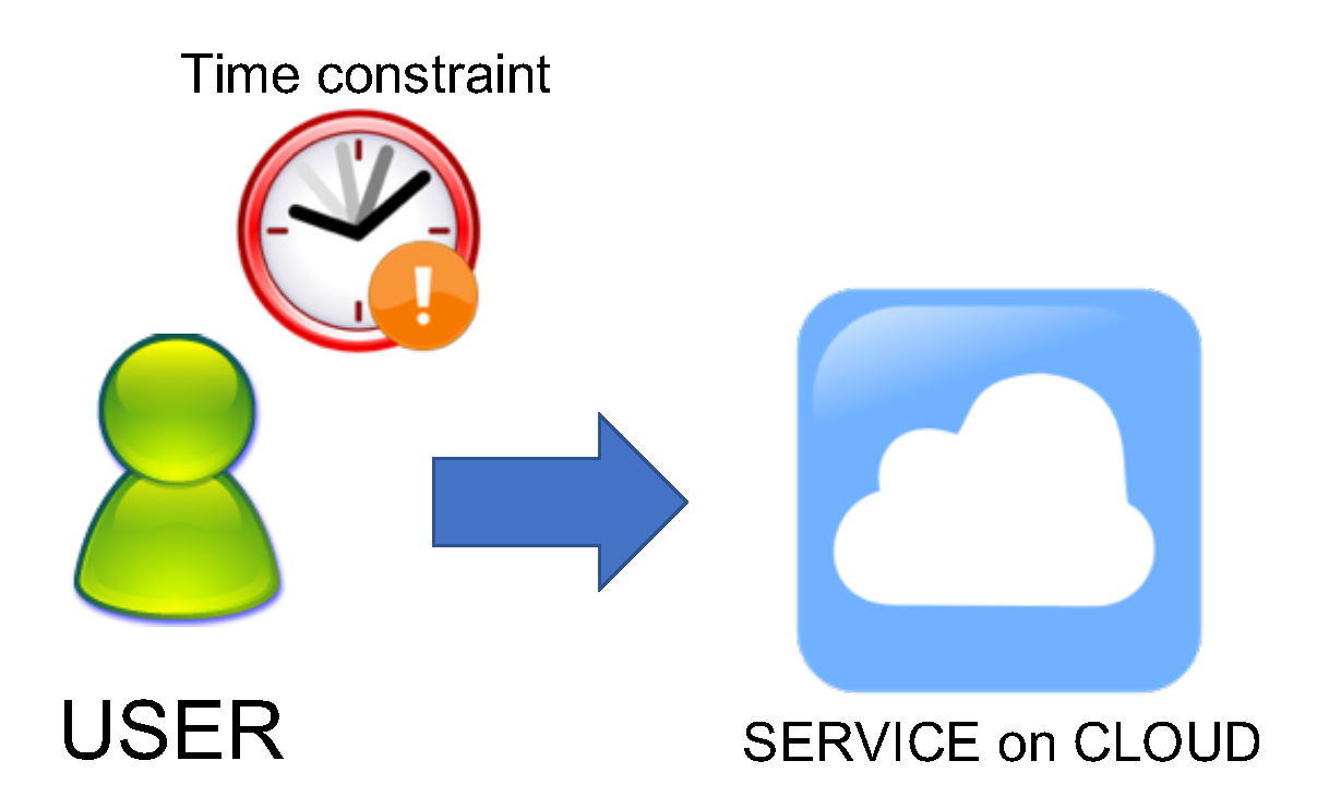
Figure 1. An application scenario including user-generated timeouts.
Futureinternet 12 00050 g001
Figure 2. Model of a cloud application with user’s timeout.
Futureinternet 12 00050 g002
Figure 3. Response times with (left) and without (right) timeout of 10 s, for λ = 1.8 r/s and K = 2 VMs.
Futureinternet 12 00050 g003
Figure 4. Distributions of response time with Timeout = 10 s and λ = 0.9 r/s for a variable number K of VMs.
Futureinternet 12 00050 g004
Figure 5. Behavior of Response Time for timeout ranging from 1 to 30 s, λ = 0.9 r/s for a variable number K of VMs.
Futureinternet 12 00050 g005
Figure 6. Trade-off between deployment cost (number K of VMs) and user satisfaction for different arrival rates λ .
Futureinternet 12 00050 g006
Figure 7. Layout of the model for the computation of the best route.
Futureinternet 12 00050 g007
Figure 8. Mean response times and 95th percentiles for the computation of the best route waiting at the Join the first k algorithms that completed their executions.
Futureinternet 12 00050 g008
Figure 9. A MapReduce application deployed on the cloud.
Futureinternet 12 00050 g009
Figure 10. Model of a MapReduce application.
Futureinternet 12 00050 g010
Figure 11. Average number of mappers (left) and reducers (right) for different number of users N and K VMs.
Futureinternet 12 00050 g011
Figure 12. Determining the optimal number of VMs to obtain an average response time R below a given threshold ( τ = 200 s in this example).
Futureinternet 12 00050 g012
Figure 13. The hybrid cloud scenario considered.
Futureinternet 12 00050 g013
Figure 14. Layout of the model for the dynamic provisioning of VM in a Hybrid cloud.
Futureinternet 12 00050 g014
Figure 15. Behavior of the number of VMs in execution in the private (a) and public (b) clouds in the interval 0–50 s. The threshold for the VMs in the private cloud is 96 and the arrival rate of requests is λ = 50 req/s.
Futureinternet 12 00050 g015
Figure 16. Number of requests in execution in the private (solid line) and public (dashed line) clouds vs. max number of VMs in the private cloud.
Futureinternet 12 00050 g016
Figure 17. Global Response time vs. maximum number of VMs in the private cloud.
Futureinternet 12 00050 g017
Figure 18. Throughput of private (solid line) and public (dashed line) cloud vs. maximum number of VMs in the private cloud.
Futureinternet 12 00050 g018
Figure 19. The considered e-Health scenario.
Futureinternet 12 00050 g019
Figure 20. Layout of the model for the smart batching of signals in the e-Health scenario considered.
Futureinternet 12 00050 g020
Figure 21. System eesponse time vs. arrival rate of requests for various values β of the batch sizes for Urgent requests.
Futureinternet 12 00050 g021
Figure 22. Batch transmissions per second vs. arrival rate of requests for various values β of the batch sizes of Urgent requests.
Futureinternet 12 00050 g022
Figure 23. System power vs. arrival rate of requests for various values β of the batch sizes of Urgent requests.
Futureinternet 12 00050 g023
Table 1. Case studies summary
ScenarioSolutionSection
Timeout with Quorum based JoinFork/Join paradigm3.1
Approximate Computing with Finite Capacity RegionFinite capacity regions3.2
MapReduce with Class SwitchClass Switch3.3
Dynamic provisioning in Hybrid CloudsMulti-formalism4.1
Batching of requests in e-Health applicationsMulti-formalism4.2
Table 2. Service demands [s], coefficients of variation, and distributions of the computation times of the six algorithms.
ComponentParameters
MeanCoeff. of Var.Distribution
Algorithm 11cv = 5hyperexp
Algorithm 23cv = 3hyperexp
Algorithm 31cv = 1exp
Algorithm 42cv = 1exp
Algorithm 54cv = 0.7Erlang
Algorithm 65cv = 0.5Erlang