1. Introduction
Among the many approaches proposed to engineer systems featuring distributed intelligence, a relevant one is
self-organization [
1], by which global structure and behavior are robustly achieved by continuous local interaction of simple individual components. This is generally meant to promote inherent adaptation to unexpected (or not completely foreseeable) contingencies, supporting applications in contexts such as human social behavior, swarm robotics, and task allocation. Therefore, in this paper we deal with artificial (software-based) self-organizing systems. Self-organization was first observed in nature, in natural systems such as ant colonies or bird flocks, and the first mechanisms for self-organization engineering were largely inspired by such systems [
1]. In recent decades, the engineering of self-organization has been widely researched in various areas including multi-agent systems [
2], autonomic computing [
3], self-managing and adaptive systems [
4], and resource management [
5]. Self-organization is generally understood as the ability of a system to sustain its internal order, in face of change and without any external control—few formalization attempts exist, e.g., via a notion of entropy of the population of system components [
6]. Often, it is common in the literature to refer to artificial systems endowing the ability to self-regulate their internal structures and behavior (e.g., by mimicking self-organization mechanisms observed in nature) as simply
self-organizing [
3,
6,
7,
8,
9]. Following this convention, in this paper we use term “self-organizing (cyber-physical) system” to mean an “artificial (cyber-physical) system featuring self-organizing logic”.
When self-organizing approaches are applied to distributed cyber-physical systems (CPS), they are essentially used to collect and process information generated by sensors distributed over the environment, and use it to control the system behavior itself [
10]—often in a purely decentralized fashion. There, individual system components form a flat space that interact with each other based on physical proximity. In these settings, direct communications with centralized servers are unpractical, expensive, or even impossible.
Recent advances in technology foster pervasiveness of computing and communication, providing opportunities for novel services and applications, which then turn into new engineering and research challenges. Current trends are making modern CPS increasingly large-scale, heterogeneous, and dynamic, requiring increasingly complex and heterogeneous infrastructures [
11]. On the one hand, remote clouds provide virtually unlimited on-demand resources (computing, storage, services), provided that costs (both in money and latency) and data protection procedures can meet the requirements of the application at hand. On the other hand, edge computing brings resources closer to users, reducing latency (increasing reactivity) and managing concerns about data dissemination. These two complementary architectures are often intertwined with other communication technologies, such as proximity interaction (e.g., Bluetooth or Near-field communication), and long-range wireless communication (e.g., Sigfox [
12] or LoRaWAN [
13]).
Such intricate and dynamic infrastructures complicate the task of solid engineering of distributed intelligent systems, whose logic tends to be significantly dependent on it. In particular, this hampers the possibility of reusing design elements across different application scenarios, and exploiting the available ICT resources opportunistically (e.g., for optimization, graceful degradation, or customization purposes). To that end, in this paper we investigate the following problem:
How to design and implement the self-organization logic of CPS in a deployment-independent way?
With “deployment-independent” we mean a separation of concerns between the self-organization logic and the deployment context. In particular, the behavioral description of the self-organization logic remains unchanged regardless of the specifics of the deployment context.
Consider as a motivating example, the problem of a smart-city CPS that consists of a computing ecosystem with devices that monitor and aggregate pollution levels and household temperatures to promote eco-friendly living. One typical approach to implement the application logic of such systems is through self-organizing algorithms—see for instance [
14]. Such algorithms employ the spatiotemporal proximity of devices to regulate the flow of information in the system in a scalable way, ultimately promoting the emergence of smart collective behavior. Evidently, such applications can be set up using different heterogeneous sets of computing and networking devices. Depending on the concrete technology at hand, the communication between physically close devices may need to be implemented in different ways, for instance, based on direct device-to-device interaction or communication via intermediaries such as fog servers or the cloud. Ideally, the application logic should not be affected by the heterogeneity of the underlying technology or the specific deployment choices (cf., cost, performance, and reliability considerations). We use this example as a case in
Section 6.
To tackle this type of problems, we propose a framework to design distributed adaptive behavior for large-scale CPSs rooted on what we call the
pulverization approach. This approach breaks the overall system behavior into tiny pieces of computation logically linked to sensors, actuators, and neighboring components, each continuously scheduled and executed across space (i.e., the computational devices available) and time.This “network” can then be smoothly mapped onto a variety of multi-layered deployment infrastructures. In other words, we provide a schema for engineering the self-organizing logic in CPSs: it is based on a flexible logical model which can be decomposed into a set of sub-components with well-defined relationships that can be deployed and wired separately (i.e., they work as “logical units of deployment”). Such a schema is to be properly instantiated and filled with details to actually drive self-organization. To that end, we show how this approach can be implemented in the framework of Aggregate Computing [
15], where global self-organizing behavior can be specified declaratively, i.e., by composing pure functions expressing increasingly complex distributed algorithms. As a key benefit, the approach can make the Aggregate Computing toolchain [
16,
17], distributed algorithms and systems [
18,
19], readily available to work in the larger class of complex ICT infrastructures [
20].
To showcase the pulverization proposal, we evaluate the approach by simulating a situated CPS, whose software components are deployed using a synergy of technologies including edge servers, low-power/long-range communication via LoRaWAN [
13], MQTT (Message Queuing Telemetry Transport) [
21,
22], and cloud offloading. We run the system over different deployment configurations, exploiting the edge and cloud layers. Then, we verify that its self-organizing logic, written once and orthogonal to the specifics of deployment, always produce the same functional behavior—although, non-functional aspects such as performance (e.g., network response time) or operating cost are affected by the underlying deployment at hand. The evaluation is performed on an evolved version of the DingNet exemplar [
23], augmented with Aggregate Computing support and features to select deployment schemes.
After discussing background and related work (
Section 2), this paper describes the following key contributions:
- 1.
A
novel model for self-organizing cyber-physical systems that fosters “pulverized” execution to realize deployment independence, formalized by a structural operational semantics defining a transition system for logical and physical network of devices (
Section 3);
- 2.
An
instantiation of the model for the aggregate computing framework (
Section 4);
- 3.
An
evaluation of the pulverization approach (
Section 6) on a simulated smart-city case comprising multiple deployments of a CPS for pollution-aware household heating control.
2. Background and Related Work
This section is structured in three parts that introduce the main related efforts and positions our work on this landscape: self-organization, decentralized self-adaptation, and flexible deployments of adaptive systems.
2.1. Self-Organization
A self-organizing system consists of (simple) components that realize the system goals through repeated local interaction. Self-organization [
24] often draws inspiration from natural systems and promotes
emergence [
25,
26], i.e., the creation of novel macro-level effects out of decentralized micro-level activity. Swarm intelligence exhibited by ants is probably the best-known example [
27]. Such macro-effects are often connected with the ability of the system to be resilient to environmental perturbations (ranging from human in-the-loop effects to faults in physical devices or communications—which are the norm in large-scale distributed systems), or to deal with changing functional/non-functional requirements that have to be satisfied in a wide variety of conditions. Relevant application of self-organization include: study of human social behavior [
28], crowd tracking and steering [
15], energy demand allocation [
29], terrain exploration [
30], smart camera coverage [
31], task allocation of autonomous vehicles [
32], and ICT resources coordination [
33].
Most of these works show a trend in self-organization, shifting from natural inspiration to the identification of “artificial” mechanisms for engineering the collective part of adaptive systems, namely to develop so-called
collective adaptive systems (CASs). Research on CASs [
34] study how a
collective (i.e., a dynamic group of “similar” autonomous entities—e.g., a swarm of robots) can support macro-level adaptivity and how such insights can be leveraged for engineering large-scale socio-technical systems.
The approach studied in this paper takes somewhat inspiration from these latter approaches, looking for ways to abstract from the actual deployment of physical systems, hence aiming to apply self-organization techniques in heterogeneous deployment settings such as those relying on multiple layers of cloud/fog/edge computing.
2.2. Decentralized Self-Adaptation
A
self-adaptive system is one that is equipped with an external feedback loop that tracks the state of the system and its environment and, through adapting it to changes, ensures that a set of goals is achieved, or if necessary, the system is gracefully degraded [
35,
36,
37,
38,
39]. In this paper, we are concerned with self-adaptive
software systems [
40] as well as their deployment, in particular cyber-physical systems.
Research on self-adaptive software relates to the field of
autonomic computing [
41]. A self-adaptive (or autonomic) system can be thought as consisting of three main pieces [
38]: (i) a
managed system, which provides the application logic and should be adapted to satisfy its requirements in different circumstances; (ii) an operating
environment, which is generally characterized by
uncertainty in terms of changes that are difficult to predict; and (iii) a
managing system, (also known as
autonomic manager [
41] or
adaptation engine [
40]), that is responsible for the management of the managed system. A common approach to realize self-adaptation is architecture-based adaptation [
37,
42,
43], which leverages architectural models of the system at runtime [
44]. The managing system is usually organized around in a feedback loop that realizes four main functions [
41]:
Monitoring,
Analysis,
Planning, and
Execution, that share common
Knowledge, MAPE-K in short.
The work presented in this paper is in particular related to
decentralized self-adaptive systems, i.e., systems in which there is not a single component responsible for adaptation, but adaptation control is distributed among multiple components [
45]. In contrast to a self-organizing system, a decentralized self-adaptive system consists of components that are equipped with feedback loops that interact locally to adapt the underlying components to realize the system goals.
Decentralization in control fosters
scalability (avoiding bottlenecks),
robustness (avoiding single points of failure), and
efficiency through the exploitation of locality (avoiding the overhead of non-local interactions). Sometimes, centralized control is simply not an option for a large class of modern distributed systems, because of cost of impact on quality attributes [
4,
46].
Despite the high relevance of decentralization of control in self-adaptive systems, existing work remains limited. We highlight a few representative approaches. Malek et al. [
47] use an auction-based coordination mechanism to find the appropriate deployment architecture under changing operating conditions. Vromant et al. [
48] extends MAPE loops with support for inter-loop and intra-loop coordination. Vogel and Giese [
49] present
EUREMA (ExecUtable RuntimE MegAmodels) that offers support for specifying interacting feedback loops models that then can be directly deployed and interpreted by an interpreter. A related, but formally founded approach is presented in [
50]. Calinescu et al. [
51] present
DECIDE (DEcentralized Control In Distributed sElf-adaptive software), an approach to decentralize feedback loops that uses quantitative verification at runtime to assure Quality-of-Service (QoS) requirements in the presence of change. The approach demonstrates better scalability compared to a centralized approach, but only for small component models.
Weyns and Georgeff [
52] apply self-adaptation in a multi-agent system application for automated guided vehicles. An example of self-adaptive middleware architecture for dynamic service composition is described in [
53], and
GoPrime [
54] offers a decentralized middleware for self-assembly of distributed services. A gossip protocol realizes decentralized data dissemination to maintain an assembly of services that fulfils global QoS goals.
Although these approaches offer complementary contributions to tackle the complex problem of decentralization of control in self-adaptation, none of these approaches targets large-scale adaptive systems nor their deployment independence, which is exactly the contribution of this paper.
2.3. Flexible Deployment
In
distributed systems, software components are deployed to hardware elements, and this affects the notion of “locality”, and the connection of computations to physical space, in ways that deserve attention. We generally refer to the hardware and the media supporting communication between hardware elements (in general, these hardware element are part of the communication network and the physical environment, where principles of stigmergy are applied [
55] to support the exchange of information of sensors and actuators) as
(ICT) infrastructure. The problem of
deployment is about how to map (components of) the system to available infrastructure. We use the same terminology of major literature [
4,
56], where term “distribution” refers to deployment and term “decentralization” refers to the degree by which
adaptation control is handled by multiple interacting components rather than by a single, central component. Notice that decentralization of control is
orthogonal to distribution (i.e., to deployment) [
4,
56]: this is indeed the main theme of this article, where we show how this principle can actually be implemented, methodologically. Though deployment is considered a research challenge for self-adaptive systems [
56], few works address the tension between application logic, adaptation control, and deployment.
Presently, infrastructure is increasingly heterogeneous, complex, and dynamic: computers range from low-powered, thin devices to large supercomputers; telecommunications technology can be wired or wireless, with many subtypes providing a wide range of capabilities and guarantees; storage and computational resources may be close, distant, or very distant to a communication endpoint—cf. edge, fog, and cloud computing; and finally, failures, interferences, replacements, extensions, can make the infrastructure dynamic. This richness is an opportunity but also a challenge for distributed computing paradigms, as typically each of them tends to address a specific deployment style.
At a first instance, applications should aim at being agnostic with respect to the underlying infrastructure and deployment. This is supported by abstraction, hiding unnecessary details for better focusing on the problem at hand, and by a middleware that makes the abstraction operational—filling the “gap” with the underlying platform or infrastructure where the details do matter.
This paper addresses the problem of identifying a suitable abstraction level to support deployment independence, or deployment agnosticism, in self-organizing systems. Instead of trying to match specific self-organizing models or patterns to the deployment at hand, we aim at a model by which general self-organizing strategies can be mapped to a variety of contexts. The key idea, inherited by approaches of so-called macro-programming [
15,
57,
58], is to consider system behavior as a conceptually global computation performed on the whole set of system devices, and being effectively independent on details such as number and (mutual) location of devices. Declarative programming approaches can naturally be applied to promote the specification of
what the computational system should perform, abstracting from concrete aspects pertaining lower-level details. Facilitated by declarativity, one such macro-behavior should then be “pulverized” into smaller pieces or chunks of behavior, each to be executed in a continuous way across “space”, i.e., across all the devices of a system. According to the self-organization principle, such chunks affect only a logical locality, in terms of perception/action over the local portion of the environment, and exchange of messages with neighbors. Deployment independence is then achieved by a suitable mapping of a general self-organization problem to the actual platform, and performed by spreading such chunks in the available devices.
Large-scale distributed and self-adaptive systems as envisioned in forthcoming CPS and the Internet-of-Things (IoT) make a case for
distributed declarative programming promoting self-organization, while at the same time leaving
degrees of freedom [
59] to designers and deployment. We highlight several representative research efforts on deployment and automatic reconfiguration of systems.
Osmotic computing [
11] is an approach to opportunistic deployment of microservices on the edge-fog-cloud platform. An osmotic platform aims to reach and maintain an “osmotic equilibrium” between infrastructural and application requirements by automatically migrating microservices to deployment locations. However, the approach mainly targets centrally orchestrated systems. Other approaches leverage component-based, architectural descriptions to decouple application logic and deployment. For instance,
DR-BIP (Dynamically Reconfigurable Behavior Interaction Priority model) [
60] and
DReAM (Dynamically Reconfigurable Architectural Modelling) [
61] use
components (capturing behavior),
connectors (capturing interaction between components’
ports),
maps (logical topologies), and
deployments (associating components to map locations), overall organized in
motifs (dynamic architectural configurations), to model and analyze dynamic architectures.
These approaches have some similarity with the approach presented in this paper, but they are arguably more complex and our approach explicitly addresses self-organizing CPS.
3. A Model of Deployment-Independent, Self-Organizing, Cyber-Physical Systems
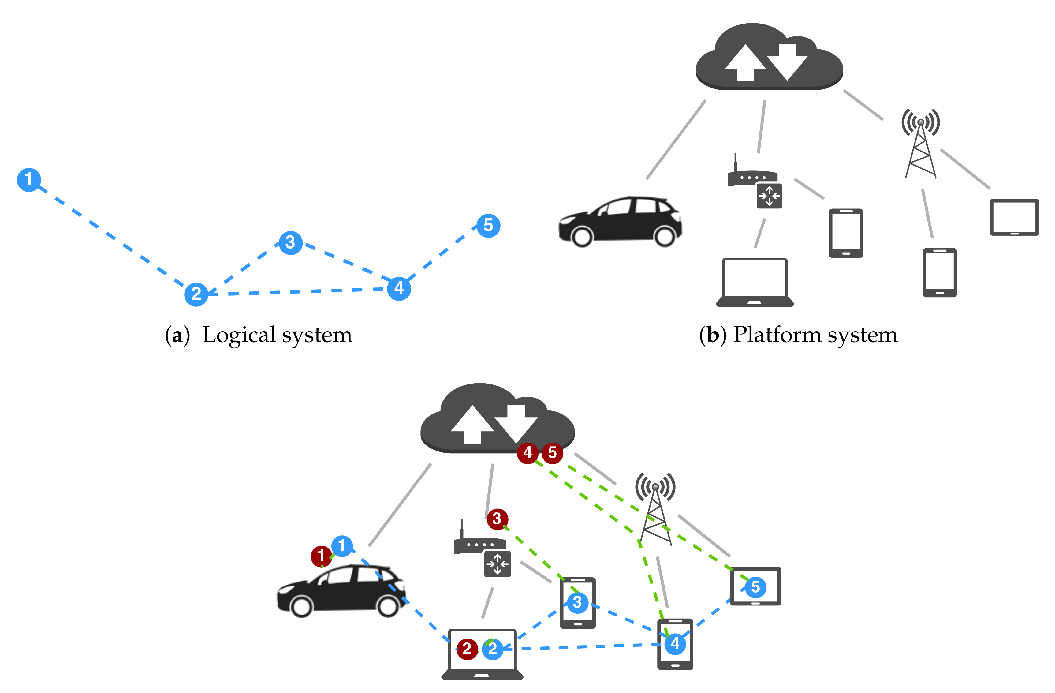
In this paper, we present an approach to conceive self-organization in distributed systems that facilitates deployment independence, i.e., the ability of an application to run with no change on various deployments while retaining its original functional semantics. It is rooted in the idea (illustrated in
Figure 1) to organize the structure and behavior of a system so that (i) the developer can focus on a logical model that mostly abstracts details concerning deployment, scheduling and communication; and (ii) the logical model can be straightforwardly partitioned into a set of deployable software components, which deployers (e.g., devops team members or automated systems) can “freely” distribute on available infrastructure. The application logic will obtain the functional goals independent of the actual deployment, yet the choice of the deployment at hand typically affects non-functional properties, such as performance and cost.
Let us consider a cyber-physical system consisting of: a
cyber system (
Section 3.1), which provides a logical model for the system; and a
platform system, which models networks of hosts for deployment (hence subsuming physical systems as well as simulation platforms) and to which the cyber system can be mapped to by a so-called
deployment (
Section 3.2). In the following, we describe this model informally at first and then formally by a structural operational semantics [
62], e.g., in the style of calculi like
-calculus [
63] (the quintessential process algebra for mobility) or the field calculus [
64] (the main foundation of aggregate computing). The main goal of the formalization, presented incrementally in the following, is to provide an unambiguous specification of what constitutes pulverization, clarify subtle aspects of the model, and state the deployment-independence property rigorously. The model will then be instantiated in the macro-programming approach of aggregate computing in
Section 4.
3.1. Cyber System
A cyber system is a collection of
logical devices (or devices for short), each with the ability of connecting to other devices, called
neighbors—generally, such connections (
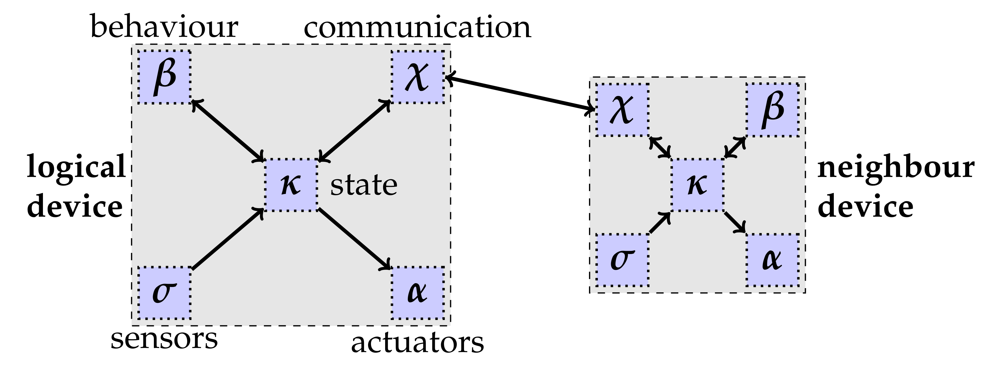
logical neighboring links) define a structure that can change over time. A device (
Figure 2) is a logical entity with the following components:
A set of logical sensors.
A set of logical actuators.
A state , representing the device’s local knowledge (where we abstract the particular representation chosen for a state).
A communication component handling interaction with neighbors, holding information on the identity of neighbors and how to reach them, managing input channels used to receive external messages into the device’s state, and output channels for emitting messages to all its neighbors (i.e., the output channel of a device is connected to the input channels of all its neighbor devices as per the neighboring relationship).
A computation function modelling the device behavior, which maps the state of the device to (i) a new state, (ii) a “prescriptive” set of actuations to be performed, and (iii) coordination messages to be emitted.
Each individual device of the cyber system performs a MAPE-like cycle that includes the following steps and that defines the interactions between the device’s subcomponents as depicted in
Figure 2 (with arrows denoting message flow).
- 1.
Context acquisition. In this step, the device retrieves information from context sources (sensors and communications) and stores them in the device state.
- 2.
Computation. The behavior function is applied against (data inferred from) the device state; its (possibly processed) output is stored in the device state.
- 3.
Coordination data propagation. From the device state, coordination data is sent to all neighbors.
- 4.
Actuation. Actuators are activated to execute a set of actions inferred from the device state (these actions are, e.g., prescribed through the device behavior or mere sensor data-driven reactions).
3.1.1. Formalization: Device Semantics
We formalize the main structure and behavioral elements of a cyber system by an operational semantics describing how the various components of a logical device interact with each other (and then how the whole logical network correspondingly evolves—
Section 3.1.2). In doing so, we specifically identify how inner components are abstracted, hence clarifying their boundary, role and interactions.
We adopt several mathematical conventions frequently used in works in process algebras [
63] and core calculi for programming languages and concurrent systems [
64], which we here briefly recap. To capture the behavior of interactive systems we use labelled transition systems [
63] which are triples
of a set
of states, a ternary relation
, and a set
of labels. We write
as a shorthand for
, meaning that the modelled system moves from state
to
by an observable action
ℓ. To describe interactive behavior we then give axioms and rules defining the triples in the relation →.
We introduce meta-variables for the various element types of the model, which are used both as non-terminal symbols in grammars and in rules of the operational semantics: we let meta-variable s range over values produced by sensors, a over values sent to actuators, x over states, e over coordination messages (also called exports) providing an internal representation of the set of messages to send/receive, i over logical device identifiers, and v over message values exchanged with other devices. We abstract away the syntax of the elements that such meta-variables range over; on the other hand, when other elements need an abstract syntax, we introduce their meta-variables by non-terminal symbols of grammars instead. As additional notation, for any meta-variable, say v, we let decorations (, , , and so on) range over the same elements as v, let be the set of elements it ranges over, be used as default value for —unless differently specified, it is assumed that different meta-variables have disjoint sets of elements they range over.
To describe the components of a cyber system we introduce the following abstract grammar:
The five kinds of components, of which only has a defined structure, are modelled as follows:
Actuators define a labelled transition system : a transition models an actuator component (generally made of a set of physical actuators) that moves from state to receiving actuation value a.
Sensors define a labelled transition system : a transition models a sensor component (generally made of a set of physical sensors) that moves from state to emitting sensor value s.
Behavior component is a pure function of the kind , namely it consumes a state, input export, and sensed value, producing a new state, output export, and actuation values.
Communication interfaces define a labelled transition system : a transition models a communication interface component that moves from state to internally receiving export e, internally producing export e, receiving message m from outside (namely from another device), and finally sending message m outward—note that an export is a general representation of neighbor values (either imported or exported), and the interface component is in charge of turning it into a set of messages for neighbors, and vice-versa.
State component is as described in the grammar: it keeps track of the status of a component, of the information useful in that status, and evolves as detailed by the rules in the following.
The semantics of a whole logical device (also called a node in this semantics) can be defined in terms of the behaviors and interactions of its logical components, which we associate to node identifiers to form
situated components. Interactions between two such situated components can produce an observable action
o:
The semantics of such interaction is given by a labelled transition system
, where
is used to mean the two situated components
interact by action
l from device
i to
moving to
. This is defined by the following rules:
That is, the node acquires context information via and in status , then computes according to its behavior , moving to status , performs actuations via , moving to status where it finally loads the export into , going back to status for another cycle. This kind of loop provides a proper pace for self-organization through MAPE-based “rounds” involving context monitoring, reasoning, and action. Notice that action is the only one involving two distinct devices i and ; in other words, all the other actions are logically local to a given device.
3.1.2. Formalization: Logical Network Semantics
On top of the formalization of interactions between pairs of situated components as presented in the previous subsection, we now define the model of a whole logical network, starting from the following grammar:
A node configuration
N is defined as a composition of components
C by operator “|”, and a logical network is defined as a composition of terms of the kind
, describing a configuration
N situated at a logical device with identifier
i. As common in process algebraic approaches [
63], we find it useful to define the network semantics first by introducing a congruence relation (i.e., an equivalence relation applicable at any level of depth), equating network configurations defined to be equivalent. This is used to define symbol “|” as multiset composition operator (associative, commutative, and absorbing configuration 0), and to allow blocks
to freely break by splitting
N; namely:
We then introduce a non-deterministic operational semantics for logical networks by the transition system
. As with transition
described in
Section 3.1.1, we write
to mean that logical network
L moves to
by executing action
l from device
i to
. As already discussed, actions of the kind
represent interaction localized inside device
i, while
with
represents an interaction through the neighboring link connecting
i to
. The transition relation is defined by the following rules:
The former two rules are standard: the first simply states that transitions work modulo the congruence relation; the second states that transitions can be applied to a network sub-part. The key rule is the third one: it selects two logical network pieces and which can interact by transition and action o, and then derives their new states and .
A logical network
L is said
complete if it is congruent to a network of the kind:
namely if every logical device
in the network has associated precisely five components, one per kind:
,
,
,
, and
. A network evolution is then defined as a sequence of transitions of the kind:
where
is complete. It is trivially shown that all
are complete, since all rules of the transition system leaves the location of components unchanged.
3.2. Platform System and Deployment as a Cyber-Physical Mapping
We represent the platform as a collection of physical hosts, connected by a possibly dynamic graph of physical network links, representing communication channels connecting a source host with a target host. A host is an entity with a network identity (e.g., a URI resource or an IP address); it can be, e.g., a computer system, a device holding a sensor, an actuator, a virtual machine, or a software container. The actual nature of the communication channel may also vary as well, depending on the network architecture and protocols. The sole relevant property is the availability of a directional channel allowing for application-level communication. Additionally, we distinguish: thin hosts, which are resource-constrained and may host sensors/actuators but not computations; from thick hosts, which instead can compute and may even do so on behalf of multiple logical devices.
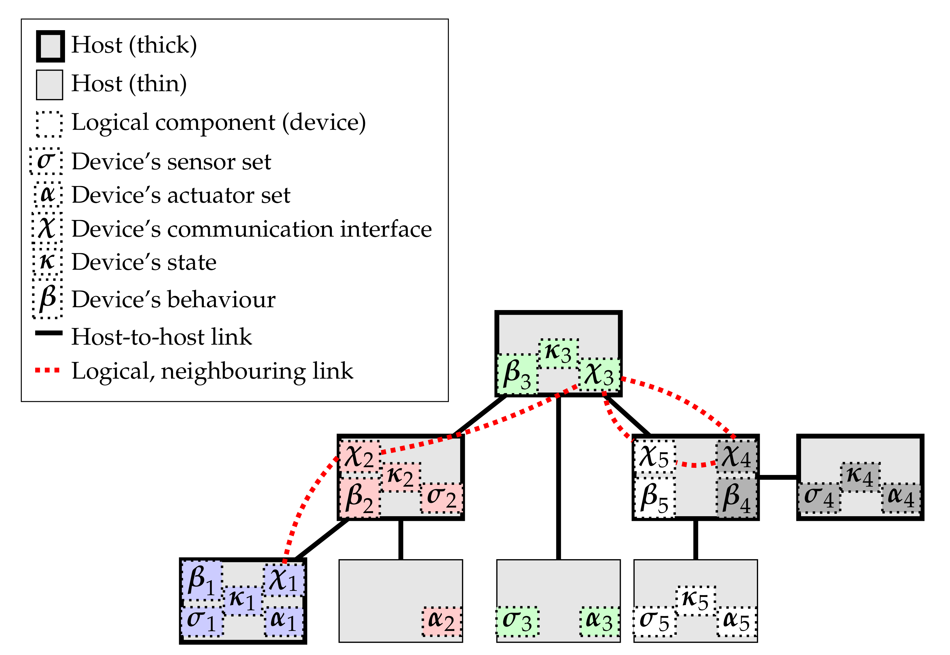
We then define a deployment as an
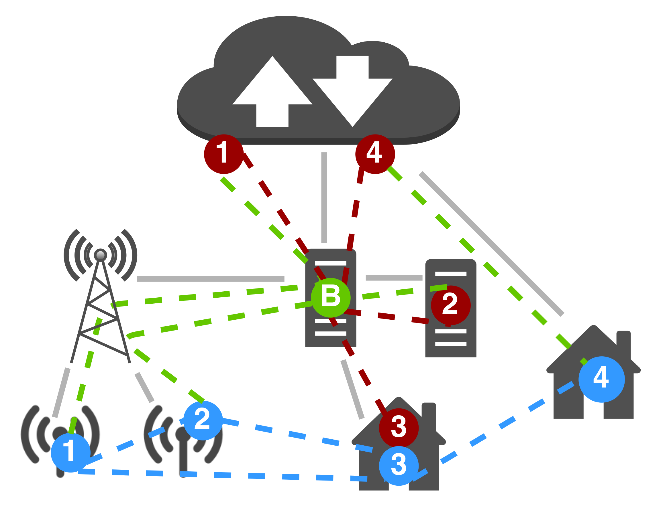
allocation map placing logical components of each device to specific hosts in the platform system, the arranging platform-level connections to support expected logical connections. An example of a deployment is pictorially shown in
Figure 3. For simplicity in presentation, we assume that all the sensors and all the actuators of a device are deployed together (into a single
- and
-component), though individual sensors and actuators may potentially be placed to different hosts. In
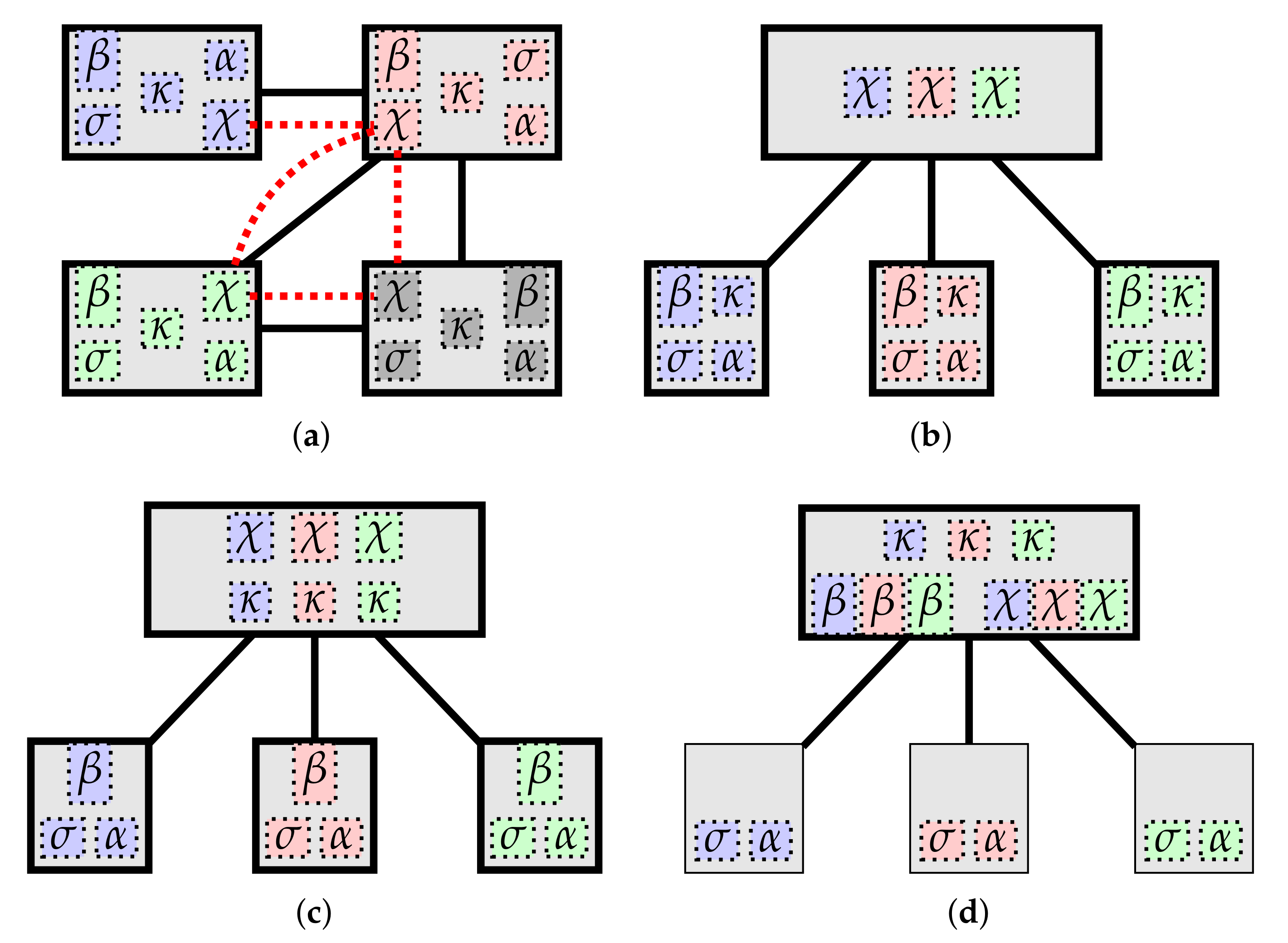
Figure 4, we provide examples of
notable deployments, showing a progression where increasing numbers of responsibilities are centralized (e.g., to a cloud or fog service layer). Of course, depending on the specifics of the actual system being deployed, some cyber-physical mappings may not be actually supported by the platform. For instance, in sensor networks whose sensing devices are designed to operate for a long time using solely battery power, such devices may not be equipped with enough computation power to host a
-component, making the deployment depicted in
Figure 4a practically unfeasible.
Details on
how to perform the mapping of a dynamic logical system upon a changing network of hosts go beyond the scope of this work. Possible approaches from literature are, e.g., in the context of
virtual network embedding [
65]. A further opportunity enabled by the proposed model is
self-(re)configuration: i.e., the autonomous process by which the platform system (re)arranges components and connections into new deployment configurations. This is a very interesting and important direction for future work.
3.2.1. Formalization: Deployed Network Semantics
We now incrementally formalize the semantics of a network deployed on a platform system. Let meta-variable
range over host identifiers (uniquely identifying physical or virtual devices being targets for deployment). A deployed network is a composition of terms
, modelling a (complete or incomplete) logical network
L located at a host with identifier
. Although evolving due to the interaction of logical components, deployed networks will then exhibit so-called
global labels, providing information on both the logical and physical links. As in previous sections, we introduce syntax
and corresponding congruence:
We then introduce a non-deterministic operational semantics for deployed networks, by the transition system
. Write
to mean that deployed network
D moves to
by executing action
l from device
i at host
to
at host
—when
and
are the same it means this is an action internal to a host, otherwise it pertains communication across a network link. The transition relation is defined by the following rules:
Again, while the former two are standard, the third is the key one, capturing the 1-to-1 correspondence with logical network evolution.
3.2.2. Formalization: Deployment
Given a deployed network
D, its corresponding logical network
can be simply obtained by erasing all sub-terms
to
L, namely:
We say that a deployed network
D is complete if its logical network
is complete. We analogously define with abuse of notation
to be the observable (logic) action obtained from global action
g erasing information about physical hosts, namely:
Definition 1. Define a deployment mapping any function such that (i) and (ii) for some . Please note that any deployment mapping is such that for any logical network L then .
Then, the following correspondence result holds.
Theorem 1. Cyber-Physical correspondence. Given a complete deployed network , for any evolution trace there exists an equivalent evolution trace in the corresponding logical network and vice-versa, such that for all k, and .
Proof. The thesis is straightforwardly proved by the way
and
have been constructed, noting that rules
D-INT and
L-INT share the same premises, and hence, if
then
and vice-versa. □
Lemma 1. Deployment independence. Given a logical network L and deployment mappings and , then the deployed networks and are such that for any evolution trace there exists an equivalent evolution trace and vice-versa, such that the corresponding logical evolutions are the same, namely for all k, and .
Proof. Straightforward. □
In this framework, the examples of mappings from
Figure 4 can be formalized as follows:
Peer-to-peer (Figure 4a). There is a bijection
such that for each
C,
.
Broker-based (Figure 4b). There is a bijection
and a
different from all
, called a
broker, such that:
and for each
,
.
State as Big Data (Figure 4c). There is a bijection
and a
different from all
, called e.g., the
cloud, such that:
,
, and for each
,
.
Cloud and thin hosts (Figure 4d). There is a bijection
and a
different from all
, called e.g., the
cloud, such that:
,
,
, and for each
,
.
4. Application to Aggregate Computing
Aggregate Computing [
15,
66] is a programming paradigm arising from the general need for capturing, linguistically and computationally, the self-organizing behavior of a (possibly large-scale, dynamic) collection of components. Its core idea is to shift from the traditional
device-centric viewpoint, which focusses on the behavior of each individual agent, to an
aggregate-centric viewpoint that emphasizes the global behavior of a
collective or
aggregate system (i.e., a whole set of interacting autonomous entities). This stance is not just conceptual, but also pragmatical: the collective logic can be expressed as an
aggregate program that is executed by an
“aggregate virtual machine” consisting of an entire (possibly distributed) system of networked agents. Aggregate programs are written in some
aggregate programming Domain-Specific Language (DSL) such as the standalone DSL
Protelis [
16] or the Scala-internal DSL
ScaFi [
17].
In this paper, we do not extend the aggregate computing model itself, but rather describe it as an instance of the model outlined in
Section 3, as follows. A logical aggregate system is a cyber system, and its deployment is an allocation map between its component and a platform system. An aggregate cyber system comprises the following elements:
Global program. All devices run the same program
. In aggregate computing, it is possible to express collective behavior through a single, global program which yields different results and actions when
interpreted against different contexts. Notice that other macro-programming languages [
67] adopt a different approach where local programs for the individual nodes are obtained by
compilation of a global program, so leading to multiple βs.
Context and Local computation. The same program is meant to be iteratively and asynchronously evaluated locally against each device’s up-to-date context, which consists of a tuple extracted from with (i) a map of the most recent sensor values for the named sensors in used by the program itself, and (ii) a map from neighbors to their most recent exported value. That is, only the last message for each neighbor is to be stored. Moreover, messages are usually retained for an application-specific amount of time. This suffices to guarantee progression and steering (via self-organization).
Program output. According to the aggregate operational semantics [
64], the output of a local execution of an aggregate program is a
vtree, i.e., a tree of values. A vtree already embeds both (i) local state to support stateful computations; (ii) information needed for coordination, to be broadcast to neighbors; and (iii) prescriptions about actuations to be performed by
. In other words, the output of an aggregate program is directly usable as an
export (see
Section 3.1.1).
Messages. Messages sent to neighbors through components are (specific parts of) vtrees.
Details about
how compositions of aggregate computing constructs give rise to self-organizing behavior are deeply covered in [
64]. It suffices to say that aggregate programs can be defined as
compositions of functional blocks that describe how a system should collectively behave through a manipulation of
computational fields [
64], i.e., dynamic maps from logical devices to computational values. However, each device computes against partial fields given by the most recent information gathered from neighbors. The key insight delivered in this paper is that the execution of such aggregate programs can be “pulverized” into micro-steps of sensing, computation, interaction, and actuation (
Section 3.1) that can also be distributed across different machines. Consider the example of a
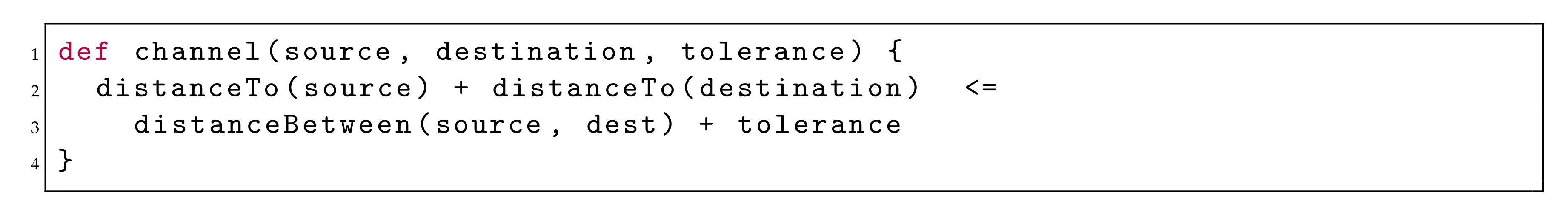
self-healing channel [
20]: an algorithm that yields, for each device, a Boolean value denoting whether it is part of the shortest path from a source to a destination group of devices, expressed in Protelis as shown in
Figure 5.
There, distanceTo(s) is a gradient (a field of minimum distances to source devices for which field s holds true) and distanceBetween(s,d) a function computing and propagating everywhere the distance between s and d. When this specification is executed in a decentralized, iterative way, it locally adapts the channel value after changes in topology, device-to-neighbor distances (obtained through a proper sensor used within distanceTo—not shown), and input fields source, destination, and tolerance. Notice how the specification is declarative: it describes the macro-level behavior without specifying exactly how micro-level behavior is to be carried out. This enables pulverization of the system, first into devices (and their execution steps) and then into devices’ components (and their execution steps). Pulverization does not depend on the specific program: the execution protocol is “fixed”; only communication payloads, which include vtrees yielded by local evaluations of the program, change. Each aggregate function call (such as distanceTo) yields a particular sub-tree including its very own relevant data.
5. Deployment Independence in Action: Aggregate Computing over DingNet
In this section, we leverage deployment independence to integrate aggregate programming, embodied by the Protelis [
16] programming language, into DingNet [
23,
68], an exemplar for research on self-adaptation in the domain of IoT.
DingNet provides an integrated simulator that maps directly to a physical IoT system deployed in the area of Leuven, Belgium. Such IoT deployment includes a situated Low-Power Wide-Area Network (LPWAN) realized with LoRaWAN devices [
13], whose hardware does not allow for intensive computation, making them obligated
thin hosts. We extend the simulator adding support for simulating edge servers and non-LoRaWAN situated devices, thus enabling controlled experiments involving a heterogeneous network composed of a mixture of thick and thin nodes whose communication intertwines several network protocols. We show how the proposed approach enables aggregate computations to be performed over such a heterogeneous infrastructure, abstracting away deployment its complexity from the business logic design.
5.1. LoRaWAN
We here briefly introduce LoRaWAN and its software stack. LoRaWAN is a communication system designed for long-range communication (up to kilometers) and low energy requirements, at the price of data rates in the order of few bytes per second (six or more orders of magnitude less than Wi-Fi or LTE). The foundational elements of LoRaWANs are end devices (or motes), gateways, and LoRa servers. Motes communicate with gateways, forming a star topology. Gateways, in turn, communicate with a LoRa server, building an overall star of stars topology. In such a network, each mote willing to communicate broadcasts its message to all nearby gateways through single hub wireless links. All the gateways receiving the packet forward it to the server through any available networking backhaul (the protocol does not govern how gateways server communicate). When communicating from servers to motes, the server selects the gateway that deems best to deliver data to the recipient. LoRa motes are designed for constrained-energy scenarios—typical industrial implementations provide battery life of 1–3 years. Consequently, motes provide little computation capacity and memory, and hence represent an exemplar case of thin devices.
5.2. MQTT-Based Network Architecture
Even though the LoRaWAN protocol focuses on communication between motes and gateways, its typical implementations usually resort to a centralized cloud LoRa server (most notably, relying on
The Things Network (
https://www.thethingsnetwork.org/) [
69]), or the
Chirpstack implementation (
https://www.chirpstack.io/)), which provides support for communicating with motes through high-level protocols, typically MQTT [
21]. MQTT is a connectivity protocol designed as a lightweight publish/subscribe messaging transport devoted to IoT and machine-to-machine communication. It defines two network entities: clients that want to exchange information; and a broker, which is in charge of receiving and redistributing data among clients. As part of the contribution of this work, we extended DingNet with an explicit model of the interaction between gateways and LoRa servers via MQTT, thus emulating the behavior of Chirpstack. The implementation has been released as open source under a permissive licence (
https://github.com/aPlacuzzi/DingNet/releases/tag/v1.3.3).
5.3. Aggregate Computing over DingNet
We now define our cyber system and the mapping of pulverized components with the platform layer given by DingNet.
The cyber system, which we target when defining the business logic, is composed of several logical devices with computation, sensing, actuation, and communication capabilities. Logical components have a position in space, and their neighborhoods are defined based on geographical proximity, within some arbitrarily chosen range (although, in principle, any policy for neighborhood definition could be used). The set of sensors and actuators may differ on each device. All logical devices have computational capabilities. Every logical device is bound to a situated platform device of the simulated system, inheriting its spatial situation.
The pulverized logical system is then mapped over the platform system as follows (see also
Table 1). Sensing and actuation systems
and
are always deployed on the host bound to the logical node. This is true for both
thin and
thick hosts. Behavior (
) and state (
) components cannot get allocated on thin hosts: their deployment targets are restricted to the cloud, edge servers, and thick situated devices. To simulate realistic situations, we allow
and
components of LoRa motes associated devices to be located solely on edge servers or on the cloud, and we let
and
associated with localized thick devices (e.g., handhelds) to be hosted locally or on the cloud. Impractical deployments, (e.g.,
and
on a device backing the LoRa mote [
70]) although possible in principle, are deemed as unrealistic with the current state-of-the-art technologies, and thus excluded from the present analysis. Moreover, as introduced in
Section 4, we note that all logical devices share the same behavior:
where
are logical device identifiers. This is part of the semantics of aggregate computing, and may vary for other pulverizable computational models. We give an example program of logical devices for the evaluation case in
Section 6. Finally, communication components
are all hosted on a single device, the MQTT broker, that can be either an edge server or a service on the cloud. This choice was made for the sake of simplicity and without loss of generality: in fact, even though in principle
components could be located on diverse hosts, and communication among them could be wired to any level 7 network protocol, we share in fact the same MQTT broker supporting the Chirpstack architecture.
Figure 6 summarizes the aggregate system as deployable within the DingNet extended simulator.
6. Evaluation
We exercise our approach for deployment independence via simulation, relying on the aforementioned extended DingNet simulator with Protelis support. In particular, we simulate a CPS whose aim is to reduce the contribution of household winter heating to air pollution [
71] by imposing custom maximum household temperatures relative to the current level of particulate matter with a diameter smaller than 10 μm (
) in the area surrounding the household.
The system must provide this functionality in a self-organizing fashion: there must be no central coordinator; rather, the system itself must autonomously organize its micro-level actuation activity, in terms of decentralized computation and interaction, so that the functionality is implemented achieved despite environmental perturbations. Our goal is to show that the same business logic, defined once, can be reused via its pulverized model across different deployment schemes, allowing the picking of an actual deployment whose non-functional tradeoffs better fit the requirements at hand.
6.1. Case Description and Simulation Configuration
Our CPS is composed of a sensor network of LoRa motes, each equipped with a sensor measuring in . Eight motes are installed in fixed position, while two are mobile (mounted on public transport systems). LoRa network coverage on the city is provided by nine gateways, whose position in the simulated environment matches one of the physical gateways deployed in the Belgian city of Leuven. The target of the control system are 300 households, randomly selected in the city area, equipped with a smart thermostat. Our logical neighborhood relationship allows logical direct communication in a unit disc of 1 km radius.
The deployment possibilities and network architecture are summarized in
Table 2. The actual deployment scheme is controlled by three parameters described in
Table 3, indicating respectively: the fraction of LoRa devices whose computation is hosted on the edge rather than on the cloud (
); the fraction of smart thermostats whose computation is hosted on the local device rather than on the cloud (
); and whether the MQTT broker is hosted on the edge or on the cloud (
B). Changing the values of such parameters generates a new deployment, with its own performance and price tradeoffs: we exercise our approach by showing that the business logic is unaffected by such change.
The DingNet simulator takes care of realistically simulating LoRaWAN network interactions and delays, while other communications are simulated with a refined version of the network model proposed by EdgeCloudSim [
72]. More precisely, the communication delay (
D) is a function of a propagation delay
d, the message size
s, and the channel data rate
b:
. Since all communications in our system are mediated by an MQTT broker, we consider delays and data rates all relative to communications from and to that broker. In particular, we assume the data rate of the broker to be
, and we compute the propagation delay
d considering the actual network path the data needs to travel, summing the individual contributions of each communication link. We account separately for end devices Internet access delay, e.g., due to Wi-Fi or LTE (
); communication delays between cloud and edge (
), edge servers (
), and cloud services (
). Actual delay values are free variables in our experiments, summarized in
Table 3. We also take into account the case in which two logically separate components are hosted on the same physical machine, in which case the data rate is considered virtually unlimited, thus
, and consequently consider such delay as constant
ms.
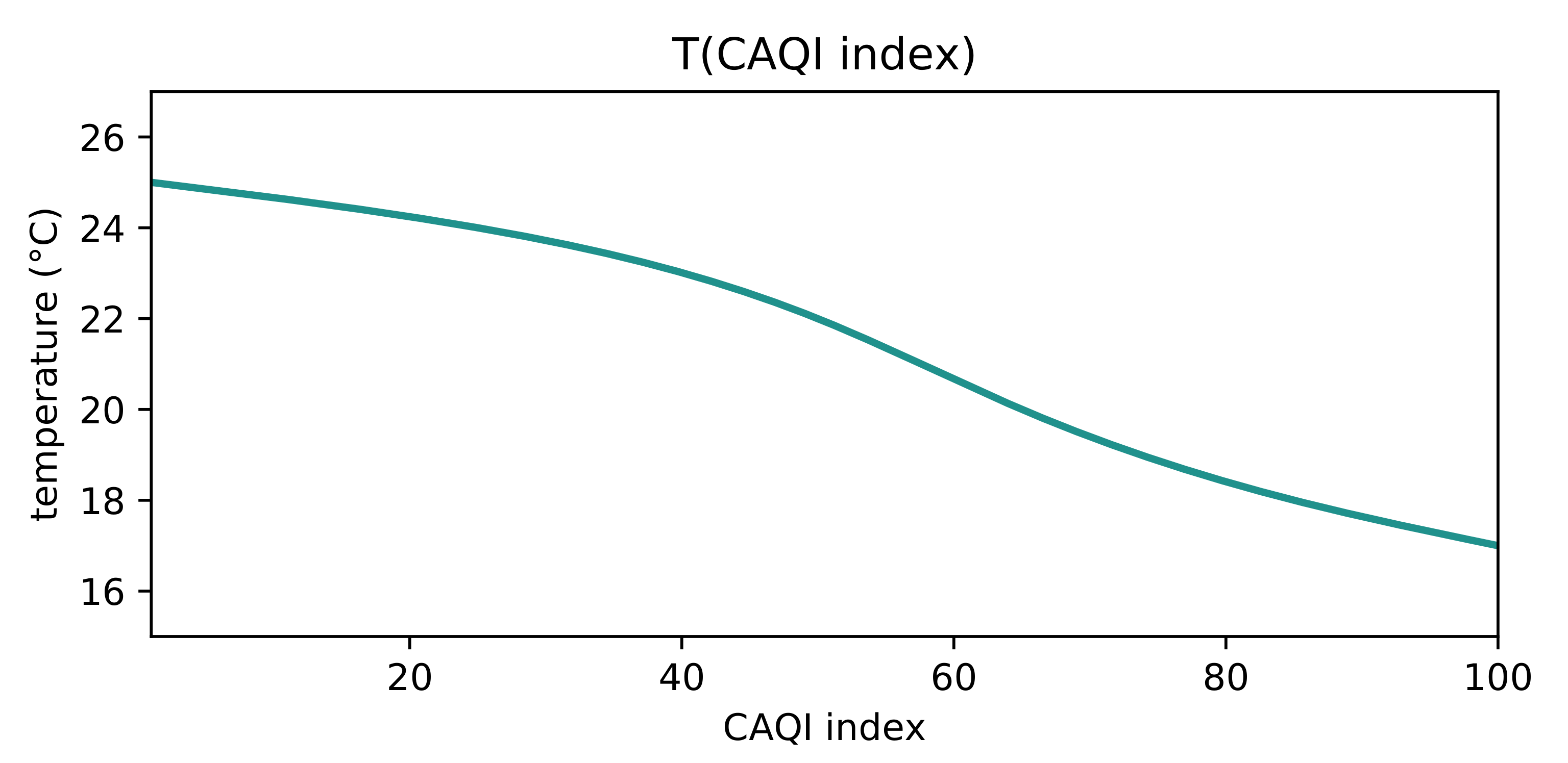
Logical devices are programmed to: (i) consider pollution data from all nodes within 2 hops; (ii) compute the local pollution value as the weighted mean of such information, using the inverse of the distance as weights; and (iii) use the value to set the maximum allowed temperature, if the appropriate actuator is available. Instead of directly relying on
as metric, it computes the CAQI index [
73], in such a way that future addition of further pollution metrics such as
can be considered with no change to behavior. The relationship between the computed CAQI index and the desired temperature used in our experiments is shown in
Figure 7.
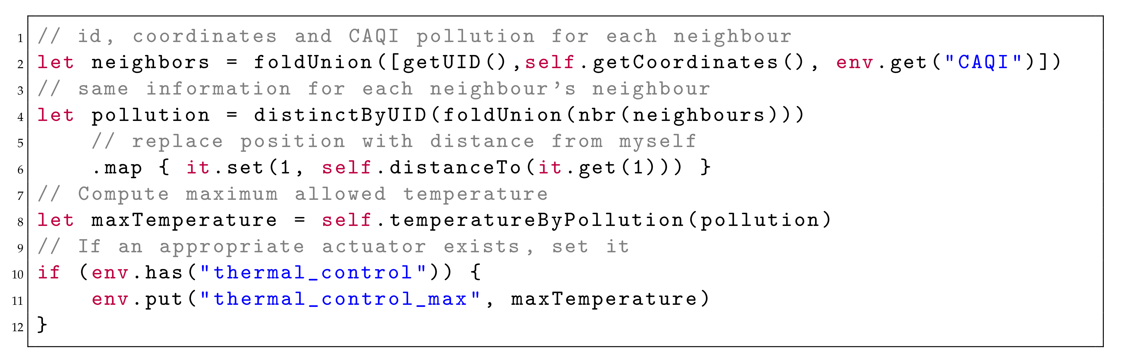
The program, excerpted in
Figure 8, is entirely independent of the actual deployment of logical devices’ components.
We simulate the system evolution over four days (96 h). Device round frequency is set to
Hz. We perturb the system by reproducing the reduction in
caused by a rainfall [
74] starting from the northern side of the city after 25 h of simulation, covering the whole city at the 31st simulated hour, and terminating at the 61st hour.
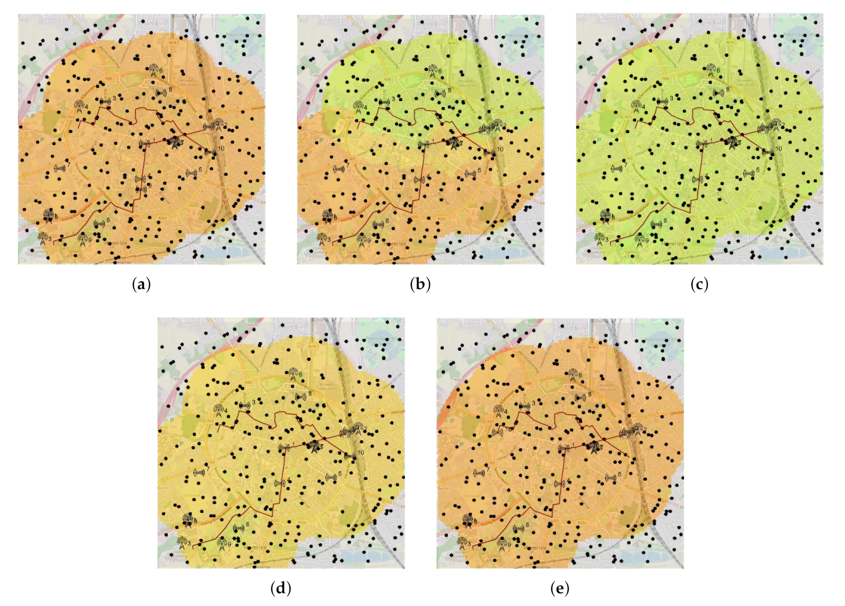
Figure 9 shows the system’s evolution through snapshots of a simulation run.
Our reference metrics are presented in
Table 4. Temperature measures are used to verify that the system is operating nominally, regardless of the deployment configuration. Latency measures are intended as a performance proxy, showcasing that different deployment choices provide different tradeoffs. We also provide an operating cost estimation for the deployment. Our estimation is the following:
We estimate the pricing for operating the MQTT broker on the cloud by referring to the prices of a prominent operator available at the time of writing (
https://archive.is/9g2tk).
We assume the broker located on the edge to be self-hosted, thus with a negligible upkeep cost.
We consider the smallest cloud server instances available from one of the major players (
https://archive.is/9fg0e). We estimate that each such instance has enough memory to comfortably host about a hundred pulverized smart thermostats.
For any cloud hosting service, we pick the pricing for the infrastructure located geographically closest to Leuven (in our case, located in Frankfurt).
We include the electricity pricing to estimate the operating cost for smart thermostats (Arguably, this cost would be charged to the end users, and thus not impact the actual operating cost directly. However, we decided to consider this negative externality in our estimation), to do so we consider them to be implemented using a Raspberry PI Zero [
75].
We execute 10 runs of the experiment with a different seed for every combination of the variables in
Table 3. Different seeds imply different household positions, users’ desired temperature, and smart device power on instant. Data analysis has been performed using Xarray [
76] and matplotlib [
77]. The complete analysis, available on the aforementioned repository, counts over 350 charts, of which the most relevant are included here.
6.2. Results and Analysis
Subsequently, we show how the pulverisation approach achieves the functional goals independently of deployment, then we elaborate on the effect of different deployments on non-functional goals, and finally we discuss threats to validity.
6.2.1. Achieving Functional Goals Independently of Deployment
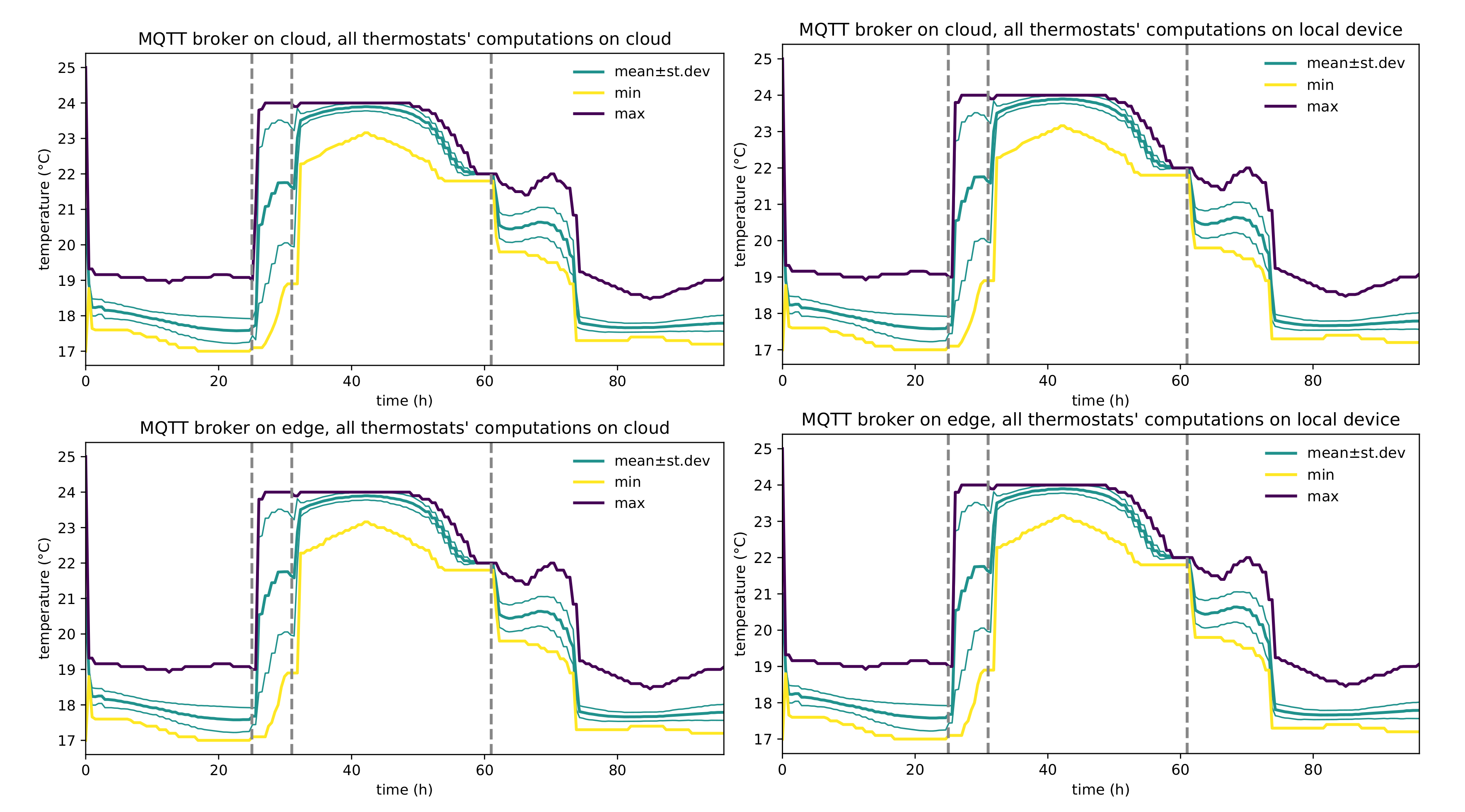
Our goal is to demonstrate that pulverization allows for reusing the same business logic on diverse deployments, thus making deployment no longer a design constraint with respect to the realization of the functionality of the system.
Figure 10 shows correctness by depicting the system functionality in a typical configuration. The system, whose overall performance changes in response to different network delays, retains its application-level behavior across the table, regardless of the actual deployment shape of its sub-components; namely the core business logic of the application is preserved regardless of the underlying deployment configuration (whose alternatives are summarized in
Table 2). The example thus shows that pulverization achieves separation between the behavior of the system from its deployment detail, thus providing flexibility to engineers that will be able to select (and change) the deployment scheme based on desired performance and projected operating cost.
We stress that no change to the application level software was required to tackle different deployment targets for any component, thus demonstrating the feasibility of a deployment-agnostic approach to self-organizing CPSs design.
6.2.2. Effect of Deployment on Non-Functional Goals
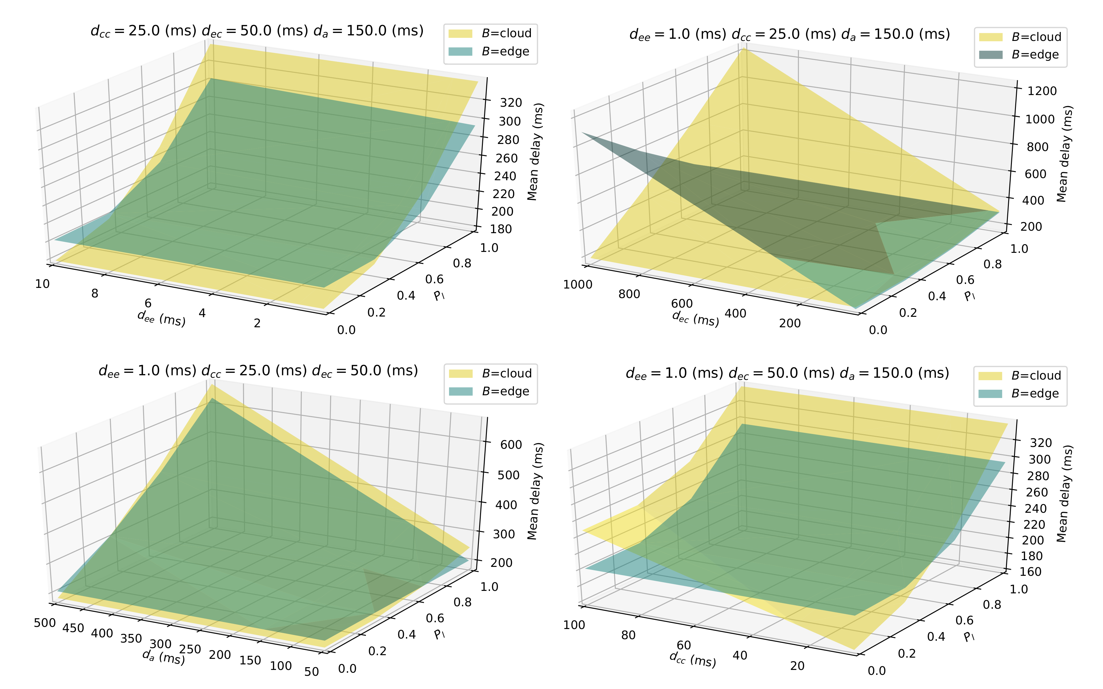
In-depth performance analysis is presented in
Figure 11, while cost estimation is depicted in
Figure 12. Performance analysis shows that depending on expected network delays, different deployment choices may have relevant performance consequences. Expressing the behavior in a deployment-independent way along with the availability of an evaluation tool enables for predicting the system’s performance across several different possibilities, thus allowing for more informed deployment choices. Should conditions change and a different deployment be required to meet performance metrics, application-level logic would not get impacted in any way.
6.3. Threats to Validity
In the section we discuss the main internal (intrinsic to the experiment, e.g., systematic error) and external (related to the generalizability) threats to the validity of the evaluation results, and for each one we explain how we mitigated it.
Regarding the correctness of the application-level behavior in the experiment: changes in the pollution level get reflected in the maximum allowed temperature setpoint for households, and the time after which the change becomes effective is subsequent to the moment sensors detect such change. Guarantees in this sense come from the structure of the application program itself. In fact, it functionally builds the output field (i.e., the field of maximum allowed temperature) through a field computation taking a single input field, namely the field of pollution level. The network performance that we measure as mean network delay, is dependent on all the free variables. For each such variable, we picked a set of values that ranges from smaller-than-normal to larger-than-normal, of course also experimenting with values that could be reasonably expected for a real deployment. To pinpoint the effect of every single variable on the performance, we execute simulation replicas for every combination in the Cartesian product of variable values, hence testing every combination. This allowed us to isolate the behavior and impact of every single change of any variable value, moreover enabling the analysis of interactions among multiple values (e.g., possible resonant phenomena).
Simulations have been performed using state-of-the-art best practices, for instance, multiple randomization-controlled simulation repetitions (ten for each combination of the free variables), guaranteeing both a reasonable problem space exploration and complete reproducibility. The first version of [
23] has been used in the past to simulate realistic LoRa communications between LoRa motes and LoRa gateways. Network communications other than those based on the LoRa protocol are modelled using a refined version of the network model proposed in [
72], as described in
Section 6.1. The most obvious threat to the validity of the network model is the lack of a model of lost packets, along with the assumption that the MQTT broker is behaving correctly and not having networking issues. In case of deployment in networks with low reliability, we expect the deployed system to show performance possibly different from the ones measured in simulation. However, we note that networking among households, edge, and cloud is usually reasonably reliable, and in our simulated system the most unreliable network is by its nature the wireless LoRa communication, whose model from Dingnet however includes packet losses, collisions, and signal propagation.
Another validity issue concerning generalisability is the resilience of the system in face of an active attacker: this kind of robustness would require specific security measures to be implemented, which fall out of the scope of this manuscript (see, e.g., [
78,
79]).
At the application level, we note that by its nature LoRa can efficiently deal with systems whose evolution in time is not exceedingly quick. If sensor readings are required multiple times per second, LoRa motes would quickly terminate their allowed use of the shared medium and hence stop transmitting to comply with the medium-use limitations [
80], hence affecting the final results. More generally, the applicability of the LoRa network architecture for the specific domain at hand puts some limitations on the generality of the results obtained for this specific case study. For similar applications in different domains, as far as time frames are similar, we expect that the simulation techniques can be straightforwardly applied. We stress, however, that such limitation is due to the specifics of LoRaWAN and affects solely the simulation platform: the concept of pulverization remains untouched, as it is conceptually independent of the network and hardware infrastructure on which we implemented it for the evaluation.
7. Conclusions and Future Work
In this paper, we introduced a novel model for self-organizing cyber-physical systems that fosters “pulverization” of the structure and execution of global system behavior (i.e., the ability to decompose macro-level components and activity into micro-level components and activities) and deployment independence (i.e., the ability of moving components and activities to different deployment targets). We then demonstrated the approach by considering an instantiation in the aggregate computing framework. We validated the approach in a simulation case of pollution-aware household heat monitoring and control, achieved through a simulator extending DingNet to support heterogeneous CPSs comprising LoRa motes, IoT devices, edge servers and Protelis nodes.
As future work, we plan to investigate and develop support for adaptive and opportunistic deployment of self-organizing systems by taking into account dynamics in the environment (for instance based on human behaviour), changes in the available infrastructure (e.g., as induced by failure and mobility), changes in requirements and preferences (e.g.,related to quality of service, operating cost, and risk), and accordingly, dynamic and opportunistic relocation of components. The theoretical framework introduced in this paper will then serve as ground.


