Abstract
This paper proposes an approach to the geospatial assessment of a territorial road network based on the fractals theory. This approach allows us to obtain quantitative values of spatial complexity for any transport network and, in contrast to the classical indicators of the transport provisions of a territory (Botcher, Henkel, Engel, Goltz, Uspensky, etc.), consider only the complexity level of the network itself, regardless of the area of the territory. The degree of complexity is measured by a fractal dimension. A method for calculating the fractal dimension based on a combination of box counting and GIS analysis is proposed. We created a geoprocessing script tool for the GIS software system ESRI ArcGIS 10.7, and a study of the spatial pattern of the transport network of the Ukraine territory, and other countries of the world, was made. The results of the study will help to better understand the different aspects of the development of transport networks, their changes over time and the impact on the socioeconomic indicators of urban development.
1. Introduction
The development of an efficient transport infrastructure is one of the most pressing problems both for the whole territory of Ukraine and for other countries. As is known, a transport system has fairly high dynamics of development, and the effectiveness of its function depends on the quality of its organization and management. The presence of a large number of diverse properties and characteristics makes it impossible and inefficient to manually process large flows of input information. This increases the relevance of the development and implementation of automated approaches and analysis tools, as well as appropriate tools for working with geodata. The best modern tool for the analysis of spatial information is geographic information technology, which combines the functionality of traditional cartography and intelligent data processing in geographic information systems (GISs) [1].
An important aspect of the application of GISs is solving environmental problems, including terrain analysis, hydrological modelling, land use analysis and modelling, ecological modelling, and ecosystem service valuation [2]. GIS techniques and procedures have an important role to play in analyzing the multicriteria decision problems of planning and management. A variety of theoretical and methodological perspectives on multicriteria decision analysis (MCDA) in GISs have been suggested over the last 20 years [3]. Examples of spatial problems that are successfully addressed by integrating MCDA and GISs are suitability multicriteria analysis and site selection analysis [4]. GIS technology can also be useful in planning the development of engineering infrastructure facilities and the construction of environmentally hazardous facilities [5]. In [6], practical examples of the use of GISs in sustainable urban planning are shown. GIS technologies allow one to observe and register changes in urban areas, manage the complex process of urban growth, and also help assess the impact of various multicriteria decision-making procedures for urban planning. Besides that, a GIS enables planners to develop and analyze urban transport development models and solve various transport-related problems.
One of the important indicators characterizing the transport system of any country is the transport provision of the territory. The transport provision level of the territory is traditionally estimated by the transport network density, the calculation of which involves using the coefficients of Botcher, Henkel, Engel, Goltz, and Uspensky [7]. A territory transport provision analysis example, based on the calculation of the Engel and Uspensky coefficients for assessing the impact of the transport system on economic security, is presented in [8]. The main drawback of the given coefficients is their use in the calculation formulas of the entire area of the territory instead of the inhabited area, which does not always adequately reflect the real picture. In order to take into account only the level of complexity of the transport network itself, and to not tie the indicator of transport provision to the area, it is proposed to calculate this indicator based on the fractals theory.
A fractal is a geometric figure that has the property of self-similarity; that is, it is composed of an infinite number of parts, each of which is similar to the whole figure [9]. The basic property of all fractal structures is their dimension. Although there is no exact definition of fractals, Mandelbrot B., the scientist who was the first to introduce the concept of fractals into science [10], gave his definition, stating that “A fractal is by definition a set for which the Hausdorff–Besicovitch dimension strictly exceeds the topological dimension” [11]. Unlike Euclidean geometry, in which dimensions are expressed in integers, the dimensions of fractal geometry can be expressed by fractional numbers between one and two in a two-dimensional space [12]. The bigger the non-integer value of the Hausdorff–Besicovitch dimension, the more irregular and complex the shape of the object.
The fractal geometry theoretical foundations development has contributed to the widespread use of fractals to describe various spatial phenomena in urban geography, urban morphology, landscape structure, and transport networks [13,14]. In [15], it was shown that the fractal geometry brings very effective apparatus to measure an object’s dimension and shape metrics in order to supply, or even substitute, other measurable characteristics of the object. Based on the fractal geographical interpretation, scientists are exploring the relationship between various aspects of urban space and the fractal dimension of cities and its changes over time [16,17]. In [18], it was shown how information on the fractal dimensions of the urban bounder and urban area can be used as a parameter for decision-making in the spatial development field, such as in the case of new residential area planning. The calculation of the fractal geometry of urban land use, performed in [19], made it possible to study the dynamics of urbanization and city expansion over recent years. Some aspects of the interpretation of the results of fractal analysis, as well as the analysis of scientific publications on the use of fractal models for urban analysis and planning, are presented in [20].
The calculation of fractal characteristics and research of the fractal pattern in the spatial structure of urban road networks provide extremely useful information for urban planning [21,22]. In particular, [23] used a modified box-counting method to describe the fractal properties of urban transportation networks and investigated the relationship between the mass size of cities and the complexity of their road systems. In [24], a box-counting method was applied to obtain a simple statistical model for determining the efficiency of filling the space of the transport system and identifying the variation in the level of fractality within the city itself and between parts of the city.
In this study, we propose a model for the geospatial assessment of the transport development of any land area based on the fractals theory. By transport development, we mean the provision of a territory with transport routes. This model will solve the problem that arises with the reliability of previous indicators that assess the level of transport development, based on the ratio of the transport network length and the territory area. Such areal indicators may give unreliable results when comparing the transport development of different countries such as, For example, the territory of Bolivia, which has an uneven population density associated with the presence of the Andean mountains, and the Amazonian jungle, which contributes to the lack of transport networks in that part of the country. Such features should be taken into account, and when calculating transport development, only the area of inhabited areas should be taken into account.
The use of the territory transport development indicator on the basis of the roads fractal dimension will allow for excluding the use of the territory area value and take into account transport network structure peculiarities by itself, while also getting a geospatial estimate of the road network complexity.
Thus, the purpose of this study is to create a model for the quantitative geospatial assessment of the territorial road network, based on the fractal dimension of roads and its implementation in the form of GIS-oriented software (scripted geoprocessing tool) for ArcMap 10.7.
2. Statement of the Problem
2.1. Classical Indicators of the Transport Provision of Territories
The concept of transport development of territories is associated with such concepts as transport provision, which reflects the quality level of transport services for facilities and the population. Obviously, the more developed the network of communication lines in a particular region, the higher these indicators are. To assess transport provision, quantitative indicators are usually used that express the ratio of the length of tracks to a unit area of a territory, or to a certain number of residents, production volumes, or other factors. For example, there are the coefficients of Engel (1), Goltz (2), and Uspensky (3) [8]:
where L is the length of the transport network in km, S is the area of the developed territory in thousands of km2, H is the total population in thousands of people, N is the number of settlements, and t is the total weight of the cargo sent to the territory.
When exploring the transport provision of a territory, it is not valid to compare the length of the transport networks with the area of the territory. It is assumed that moving away from the areal component and analyzing the level of complexity of the transport network itself may become more rational. A good example is a study of the calculation of the transport provision of a territory based on the theory of fractals, which is displayed in [25]. In contrast to the indicators in Equations (1)–(3), an indicator based on the fractal dimension excludes the area of the territory and takes into account the structural features and complexity of the road network itself, where the fractal dimension of each cell of the territory reflects a certain level of its density of the road network.
2.2. Calculation of the Transport Provision of Territories Based on the Fractals Theory
It is known that the Hausdorff–Besicovitch dimension is a natural way to determine the dimension of a subset in metric space. In three-dimensional Euclidean space, the Hausdorff–Besicovitch dimension of a finite set is zero, the dimension of a smooth curve is one, the dimension of a smooth surface is two, and the dimension of a set of nonzero volume is three. For more complex (fractal) sets, the Hausdorff–Besicovitch dimension may not be an integer [26].
The determination of the Hausdorff–Besicovitch dimension can be considered by measuring the dimension of a curve (Figure 1), which is covered by a fixed grid of squares with a side ε > 0. Each point of a linear object belongs to one of the squares. Squares in which there are no points are not taken into account. The sum over all the squares covering the object (Hausdorff measure) has the following form:
where p is an arbitrary parameter.
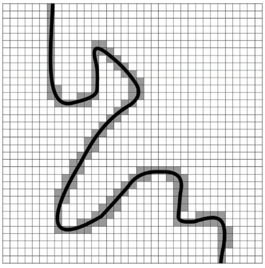
Figure 1.
Determination of the Hausdorff–Besicovitch dimension using the ε coating.
There is a critical value of p0 such that for all p < p0 and for all p > p0. This value p0 = DH is the value of the Hausdorff–Besicovitch dimension.
For example, for a square Q having a unit size with ε = 1/10, the number of square boxes covering Q equals N (ε) = ε−2 = (1/10)−2 = 100. The Hausdorff measure is mp (Q) = N(ε)εp = εp−2. Let us say ε → 0. Then, mp (Q) → ∞ for all p < 2, and mp (Q) → 0 for all p > 2. Thus, DH (Q) = DimQ = 2.
The dimension in general is determined by the law of similarity:
By taking the logarithm of the right and left sides of Equation (5), we obtain
where N(ε) is minimal number of the square boxes covering the object and ε is the square box size.
Let us give a definition of the transport provision of the territory based on the fractals theory [20].
We will consider the geospace (territory) as a two-dimensional space, and the maximum transport provision of the territory is the possibility of getting from each point of this territory to any other point in the shortest distance.
By destination points, we mean areal objects (points) whose dimensions (area) in this scale of research are negligible. Then, any territory can be represented as a finite number of such areal objects on a certain scale. A hit at any point of the area of the object is equivalent to falling into its center.
Since it is necessary to cover with points the entire investigated territory, it is advisable to choose the corresponding figure, a hexagon, as an area object. Thus, the transport development of the territory will be at a maximum when all the centers of the hexagons are interconnected by faces (a linear object) (Figure 2). These line features are actually roads on a territory map.
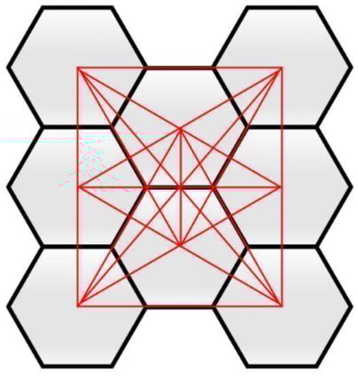
Figure 2.
An example of maximum transport provision of territories.
Since any line to a certain scale is a fractal, the transport provision of the territory can be understood as the desire of the roads to occupy the entire area on which they are located. Therefore, the level of transport provision of the territory (TP) can be represented as the ratio of the fractal dimension of the studied road to the dimension of the area (equal to 2) or, taking into account Equation (7) [25], this can be expressed as
3. The Main Research
3.1. Research Methodology
The research methodology provided for the development of a model for the geospatial assessment of a territory’s transport development is based on the fractals theory, in accordance with Equations (7) and (8).
In this study, the box-counting method was used to calculate the fractal dimension [9,27]. The essence of the method is as follows. The original dataset was split into a square box of size ε as a fixed grid (Figure 1). Next, the minimum number of square boxes N (ε) that cover the original object was calculated. Calculations of N(ε) were performed for various sizes of ε. For a small ε value, the square box number should behave like ~ε−D, and in this case, logN(ε) = D⋅log1/ε. According to the data obtained, we constructed a dependence of the following form:
Then, we calculated its slope d, defined as
To find the slope of Equation (8) in logarithmic scale, we had to build the general linear regression, expressed in the following form:
where Δ represents the error of a linear approximation.
The transport development of the territory was calculated as the ratio of the studied road dimension to the area dimension (i.e., a dimension equal to 2), based on Equation (8).
To implement the model, was created a Python script that calculated the fractal dimension for a polyline shapefile with a road network in the ArcMap program of the ArcGIS platform. In accordance with the proposed model, the study area was covered with a network of hexagons of a given size. Then, using the box-counting method, the road network fractal dimension and the territory transport development within each hexagon were calculated, as in Equation (8).
The script execution result was a polygonal shapefile, the attribute table of which had a numerical field added with the territory transport development’s calculated value for each polygonal object (hexagon).
As they were required for the script to work, base maps of the administrative area (boundary) and the road network were imported from the OpenStreetMap dataset in .shp format [28].
Modeling was performed for the following countries: Ukraine, Germany, and Bolivia. To compare their transport development level values, the same hexagon size was chosen, equal to 1000 km2, so that most settlements had a single transport development and did not introduce additional errors into the study on the selected scale of countries. In the attributive tables of polyline layers of the road networks of countries, using an SQL query, only major trunk roads of international and regional importance were selected. These polyline features are tagged with highway = (motorway; trunk; primary; secondary).
Testing of the script was also carried out for a large-scale map, representing the territory of the city of Odessa (Ukraine). All road types were considered, including streets and roads within residential areas. The hexagon area was chosen as 0.25 km2. The results obtained made it possible to compare the network fractal dimension indicators within the same settlement.
3.2. Results
For geospatial assessment of the transport provision of territories, a geoprocessing tool was created: an autonomous Python script that allowed one to calculate the fractal dimension for vector geodata with a linear geometry type.
ArcGIS contains a large library of geoprocessing tools for spatial modeling and the analysis of geographic data. The tools are grouped into toolboxes by the type of actions they perform (e.g., 3D Analyst, Spatial Analysis, and Cartography) [29,30]. To provide access to all standard ArcGIS geoprocessing tools via Python code, the ArcPy library was imported. In addition, the NumPy and SciPy libraries were imported into the script, allowing the use of high-level mathematical functions with data arrays, including data linear approximation [31,32].
Two inputs to the script were entered: a polygon shapefile with the administrative boundary of the study area and a polyline shapefile with the road network (Figure 3). In addition, it was necessary to indicate the area scale for fractal analysis (i.e., the area of one hexagon on the ground).
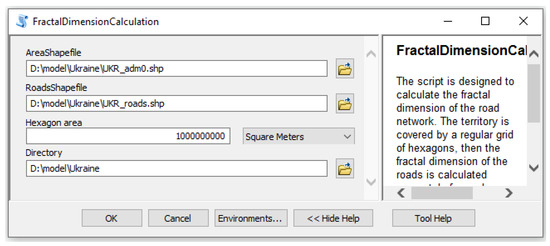
Figure 3.
Python script interface.
When running the script using the GenerateTessellation() tool, a polygon shapefile (Hexagons.shp) was created with regular hexagons of a given area (Figure 4), which covered the study area and was then used to calculate the fractal dimension of the roads. The attribute table of this layer contained an ID column with a unique code for each hexagon object.
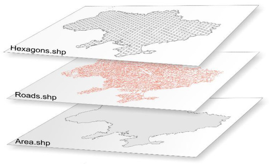
Figure 4.
Hexagon polygon shapefile covering the study area.
Using the Intersect() tool, the intersection of linear objects of the Roads.shp road network with the Hexagons.shp hexagon layer was performed. According to these results, each section of the road was assigned the ID of the hexagon in which it was located. The combination of road sections belonging to one hexagon into a single object that had an ID that matched the hexagon ID was performed using the Dissolve() tool. The resulting polyline shapefile would then be used in a script called HexagonsDiss.shp.
The calculation of the fractal dimension was carried out in a cycle for each polygonal object from the Hexagons.shp attribute table. In each iteration of the cycle, using the CreateFishnet() tool, a grid was constructed with the cell size ε, and the number of squares N(ε) that covered all linear objects (roads) inside the current hexagon was calculated.
Calculations of N(ε) were carried out for various values of ε. There were five steps. Each hexagon was covered by a grid with 1, 4, 16, 64, and 256 squares, and the size of the square decreased by 1, 2, 4, 8, and 16 times, respectively (Figure 5).
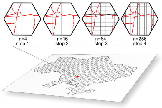
Figure 5.
Steps for executing the box-counting method.
The calculation of the fractal dimension was carried out using linear approximation by the method of least squares. As an estimate of the fractal dimension, the slope value of the straight line was used. The following is a fragment of the program code for a script that calculates the coefficients α and β of the linear function in Equation (10) using the least squares method:
#Target function
fitfunc = lambda p, x: (p[0] + p[1] ∗ x)
#Distance to the target function
errfunc = lambda p, x, y: (fitfunc(p, x) − y)
#Minimize the sum of squares of a set of equations; p1 = [α,β]
p1,success = optimize.leastsq(errfunc, [0,0], args = (logx, logy))
For the example shown in Figure 5, changes to N(ε) as a function of ε are given in Table 1. The regression line to estimate the fractal dimension is shown in Figure 6.

Table 1.
The change of N(ε) versus different values of ε for the example in Figure 5.
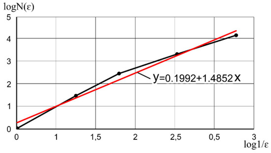
Figure 6.
The regression line to estimate the fractal dimension.
After performing linear regression, an equation of the following form was obtained: ln(N(ε)) = 0.1992 + 1.4852ln(1/ε) + Δ. The slope of this curve is equal to the box-counting dimension d = 1.4852. Accordingly, the level of transport provision, in accordance with Equation (11), is equal to TP = 1.4852/2 = 0.7426.
Figure 7 shows examples of roads of various fractal geometries and the values of the indicator of transport provision of the territory calculated for them.
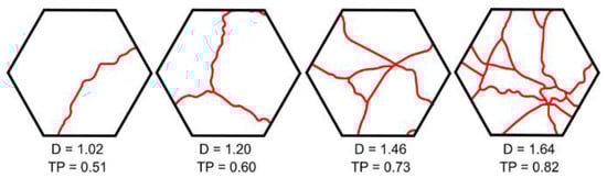
Figure 7.
Fractal dimensions and transport utilization rates for different road patterns.
The script operation algorithm is shown in Figure 8. The result of the script was a vector layer of hexagons, the attribute table of which contained calculated values of the level of transport provision for each hexagon in the TP field. The resulting value fell in a range from zero to one.
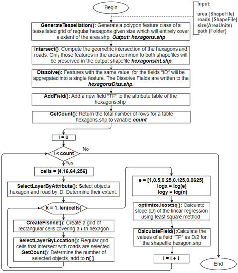
Figure 8.
Python script algorithm.
4. Discussion
Using the created script, as an example of use, a map of the transport provision of Ukraine was constructed, shown in Figure 9.
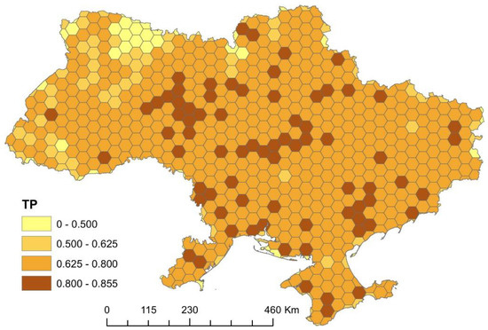
Figure 9.
Ukraine road network transport provision level.
The area of the hexagonal cell of the fixed grid was chosen, equal to 1000 km2. The resulting vector map, consisting of 710 polygon features, was classified by the TP field, which contained the calculated values of the transport provision indicator in accordance with Equation (11).
The script execution time was 44 m 54 s. For simulation, a PC with modest technical characteristics was used: an Intel Pentium Processor G4400 (3 M Cache, 3.30 GHz) with an Intel HD Graphics 510 integrated graphics processor, 4.00 Gb DDR4 RAM, and an Asus H110M-K motherboard. When using a PC with better performance, one should expect a reduction in script execution time.
In the territory of Ukraine, low values of fractal dimensions are observed in the absence of settlements and an increase in its values in the vicinity of cities. At the same time, the relationship between the size of the population of the city and the growth of the area with a high fractal dimension index around it is clearly traced.
In percentage terms, in 11% of the Ukraine territory, transport provision is less than 0.5 (very low value with a sparse road network). In 14%, the level of transport provision is from 0.5 to 0.625 (low value with a sparse road network; that is, there are single primary roads crossing the territory). In 63%, the value of the indicator is from 0.625 to 0.8 (average value; that is, there is a network of primary roads between settlements). Lastly, in 12%, a high level of transport provision appears in a range from 0.8 to 0.855.
If we compare the transport provision of different countries around the world, we can see the relationship between the population density and the growth of the territory with a high fractal dimension index. In Figure 10, (a) shows the result of calculating the transport provision of Bolivia, located on the continent of South America, which has a low population density, and (b) shows Germany, a country in Europe with a high population density. The area of the hexagonal cell of the fixed grid was also chosen to be 1000 km2. The simulation results are presented in Table 2. In 61% of Bolivia’s territory, the indicator of transport provision is less than 0.5, including 47% of the territory that lacks a road network (i.e., the indicator is zero). This is due to the presence of large areas of Amazonian rainforests in this part of the country. The Bolivia territory is also crossed by the Andean mountains, which contributes to the scarcity of transportation lines. In the remaining 39% of the territory, various values of transport provision are observed, with a predominance of values in the range from 0.5 to 0.79. As for Germany, about 79% of its territory has a transport provision index above 0.625, including 34% above 0.75.
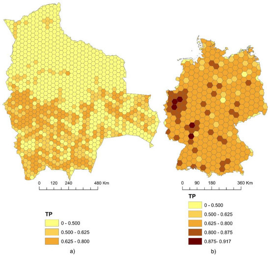
Figure 10.
The level of transport provision of the territory (a) for Bolivia and (b) for Germany.
Table 2.
Comparative characteristics of the calculation of transport development of a territory.
Table 2 shows the comparative characteristics of the calculation of the transport provision of a territory for different countries. We also presented these countries’ transport network density values, calculated as the highway length ratio to the territory area, and the values of Engel’s coefficient, in accordance with Equation (1). Although it is not possible to compare the indicators of transport development calculated using Engel’s coefficient (generalized indicator) and the fractal method (geospatial indicator), the main differences are still visible. The transport development of the territory of Germany, based on the value of Engel’s coefficient (8.3), is almost 1.7 times less than the transport development of the territory of Ukraine (14.3) and is practically equal to the transport development of Bolivia (8.8). However, as can be seen in Figure 9 and Figure 10, the values of transport development in Germany in most of the territory, calculated by the fractal method, have medium and high values, reaching 0.917 in individual hexagons, while for Ukraine, the maximum transport development value does not exceed 0.855.
The transport network fractal dimension calculation, in accordance with the proposed algorithm, can be performed for any land area, such as cities and towns. In this case, when using larger scale maps, one should choose a smaller hexagon size. Figure 11 shows the result of modeling the fractal dimension for the city of Odessa (Ukraine), the area of which is 163 km2. The data source is the OpenStreetMap map service. All road types were considered, including streets and roads within residential areas. The hexagon area was 0.25 km2.
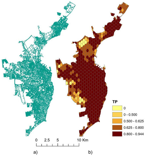
Figure 11.
Modeling results for the territory of the city of Odessa, showing (a) the transport network and (b) the transport development level.
The obtained modeling results (Figure 11b) allowed us to identify differences in the level of fractality within the city itself and compare the transport development indicator between parts of the city. A high or very high level of transport development (0.8–0.94) was found for the central and coastal regions, the most inhabited areas of the city of Odessa, while the suburban areas had a low level of transport development (0.5–0.625).
5. Conclusions
This paper proposes a geospatial approach to the study of transport provision based on the fractal dimension of roads, which allows one to obtain quantitative values of provision (level of spatial complexity) for a road network of any land territory. An algorithm for calculating the fractal dimension of roads based on the box-counting method was developed, and a scripted geoprocessing tool for ESRI ArcGIS 10.5 was created. The Python code for the FractalDimensionCalculation script has been uploaded to the GitHub repository, available to download for free (https://github.com/kuznichenko-s/FractalDimension).
Using the developed script, a study of the density of the road networks of the territory of Ukraine and other countries of the world was carried out. Additionally, the script was used to study urban and suburban areas (for example, the city of Odessa). The resulting map of the geospatial assessment of the transport development indicator made it possible to identify differences in the level of fractality within the city itself and compare the indicator of transport development between parts of the city.
The proposed quantitative model and script can be useful for scientists studying urban transport networks, in order to analyze the dynamics of their change over time, as well as to compare the level of complexity of transport networks in individual urban areas and their impact on socioeconomic indicators of urban development.
Given the high computational complexity of the algorithm, the development of parallel algorithms for calculating the fractal dimension (for example, on GPUs) can be a vector of subsequent research in this direction.
Author Contributions
Conceptualization, M.K., S.K., N.K., O.F.-F. and D.J.; Formal analysis, M.K. and D.J.; Methodology, M.K., S.K., N.K., O.F.-F. and D.J.; Software, S.K., N.K. and O.F.-F. All authors have read and agreed to the published version of the manuscript.
Funding
This research received no external funding.
Conflicts of Interest
The authors declare no conflict of interest.
References
- Hanks, R.R. Encyclopedia of Geography Terms, Themes, and Concepts; ABC-CLIO: Santa Barbara, CA, USA, 2011; p. 405. [Google Scholar]
- Zhu, X. GIS for Environmental Applications a Practical Approach; Swales & Willis Ltd.: Exeter, Devon, UK, 2016; p. 471. [Google Scholar]
- Maliene, V.; Grigonis, V.; Palevičius, V.; Griffiths, S. Geographic information system: Old principles with new capabilities. Urban Des. Int. 2011, 16, 1–6. [Google Scholar] [CrossRef]
- Malczewski, J.; Rinner, C. Multicriteria Decision Analysis in Geographic Information Science; Springer: New York, NY, USA, 2015; p. 331. [Google Scholar] [CrossRef]
- Kuznichenko, S.; Buchynska, I.; Kovalenko, L.; Gunchenko, Y. Suitable site selection using two-stage GIS-based fuzzy multi-criteria decision analysis. In Advances in Intelligent Systems and Computing; Springer: Cham, Switzerland, 2020. [Google Scholar]
- Kuznichenko, S.; Kovalenko, L.; Buchynska, I.; Gunchenko, Y. Development of a multi-criteria model for making decisions on the location of solid waste landfills. East. Eur. J. Enterp. Technol. 2018, 2, 21–31. [Google Scholar] [CrossRef][Green Version]
- Kozhevnikov, S.A. Spatial and territorial development of the European North: Trends and priorities of transformation. Econ. Soc. Chang. Facts Trends 2019, 12, 91–109. [Google Scholar] [CrossRef]
- Plotnikov, V.; Makarov, I.; Shamrina, I.; Shirokova, O. Transport development as a factor in the economic security of regions and cities. In Proceedings of the TPACEE-2018. E3S Web of Conferences, Moscow, Russia, 3–5 December 2018; Volume 91, p. 05032. [Google Scholar] [CrossRef]
- Falconer, K. Fractal Geometry: Mathematical Foundations and Applications, 3rd ed.; Wiley: Chichester, UK, 2014; p. 400. [Google Scholar]
- Mandelbrot, B. How long is the coast of Britain? Statistical self-similarity and fractional dimension. Science 1967, 156, 636–638. [Google Scholar] [CrossRef] [PubMed]
- Mandelbrot, B. The Fractal Geometry of Nature; W.H. Freeman and Company: New York, NY, USA, 1982; p. 15. [Google Scholar]
- Barnsley, M.F.; Rising, H. Fractals Everywhere; Academic Press Professional: Boston, MA, USA, 1993. [Google Scholar]
- Frankhauser, P.; Pumain, D. Fractals and Geography. In Models in Spatial Analysis; ISTE Ltd.: London, UK, 2007. [Google Scholar]
- Jiang, B.; Brandt, S. A fractal perspective on scale in geography. Isprs Int. J. Geoinf. 2016, 5, 95. [Google Scholar] [CrossRef]
- Pastzo, V.; Marek, L.; Tucek, P.; Janoska, Z. Perspectives of fractal geometry in GIS analysis. GIS Ostrav. 2011, 1, 232–236. [Google Scholar]
- Batty, M.; Longley, P.A. Fractal Cities: A Geometry of Form and Function; Academic Press Inc.: San Diego, CA, USA, 1994. [Google Scholar]
- Shen, G. Fractal dimension and fractal growth of urbanized areas. Int. J. Geogr. Inf. Sci. 2002, 16, 419–437. [Google Scholar] [CrossRef]
- Jevric, M.; Romanovich, M. Fractal Dimensions of Urban Border as a Criterion for Space Management. Procedia Eng. 2016, 165, 1478–1482. [Google Scholar] [CrossRef]
- Chen, Y. Defining urban and rural regions by multifractal spectrums of urbanization. Fractals 2016, 24, 1650004. [Google Scholar] [CrossRef]
- Purevtseren, M.; Tsegmid, B.; Indra, M.; Sugar, M. The fractal geometry of urban land use: The case of Ulaanbaatar city, Mongolia. Land 2018, 7, 67. [Google Scholar] [CrossRef]
- Wang, H.; Luo, S.; Luo, T. Fractal characteristics of urban surface transit and road networks: Case study of Strasbourg, France. Adv. Mech. Eng. 2017, 9. [Google Scholar] [CrossRef]
- Sun, Z.; Zheng, J.; Hu, H. Fractal pattern in spatial structure of urban road networks. Int. J. Mod. Phys. 2012, 26. [Google Scholar] [CrossRef]
- Lu, Y.; Tang, J. Fractal dimension of a transportation network and its relationship with urban growth: A study of the Dallas—Fort Worth area. Environ. Plan. B Plan. Des. 2004, 31, 895–911. [Google Scholar] [CrossRef]
- Sreelekha, M.G.; Krishnamurthy, K.; Anjaneyulu, M.V.L.R. Fractal Assessment of Road Transport System. Eur. Transp. 2017, 5, 65. [Google Scholar]
- Korolev, A.; Yablokov, V. The Model of Transport Development of the Territory Based on the Theory of Fractals; Regional Studies; Publishing House of the Smolensk Humanitarian University: Smolensk, Russia, 2014; pp. 29–34. [Google Scholar]
- Feder, J. Fractals; Plenum Press: New York, NY, USA, 1989. [Google Scholar]
- Robinson, J.C. Dimensions, Embeddings, and Attractors; Cambridge University Press: New York, NY, USA, 2011; p. 205. [Google Scholar]
- Arsanjani, J.J.; Zipf, A.; Mooney, P.; Helbich, M. An Introduction to OpenStreetMap in Geographic Snformation Science: Experiences, Research, and Applications; Springer International Publishing: Cham, Switzerland, 2015; p. 324. [Google Scholar] [CrossRef]
- Tateosian, L. Python for ArcGIS; Springer: Cham, Switzerland; Heidelberg, Germany; New York, NY, USA; Dordrecht, The Netherlands; London, UK, 2015; p. 544. [Google Scholar]
- Lawhead, J. Learning Geospatial Analysis with Python, 3rd ed.; Packt Publishing Ltd.: Birmingham, UK, 2019; p. 447. [Google Scholar]
- Bressert, E. SciPy and NumPy: An Overview for Developers; O’Reilly Media: Sebastopol, CA, USA, 2012; p. 68. ISBN 1449305466. [Google Scholar]
- SciPy Community. SciPy Reference Guide Release 1.0.0. 2017. Available online: https://docs.scipy.org/doc/scipy-1.0.0/scipy-ref-1.0.0.pdf (accessed on 15 November 2020).
Publisher’s Note: MDPI stays neutral with regard to jurisdictional claims in published maps and institutional affiliations. |
© 2020 by the authors. Licensee MDPI, Basel, Switzerland. This article is an open access article distributed under the terms and conditions of the Creative Commons Attribution (CC BY) license (http://creativecommons.org/licenses/by/4.0/).