Tooth-Marked Tongue Recognition Using Gradient-Weighted Class Activation Maps


Abstract
1. Introdution
2. Related Work
2.1. Tongue Diagnosis
2.2. Visual Explanation
3. Method
3.1. Problem Formulation
3.2. Model Architecture
4. Experiment and Discussion
4.1. Dataset
4.2. Training
4.3. Test
4.4. Comparison
4.5. Effects of Parameters
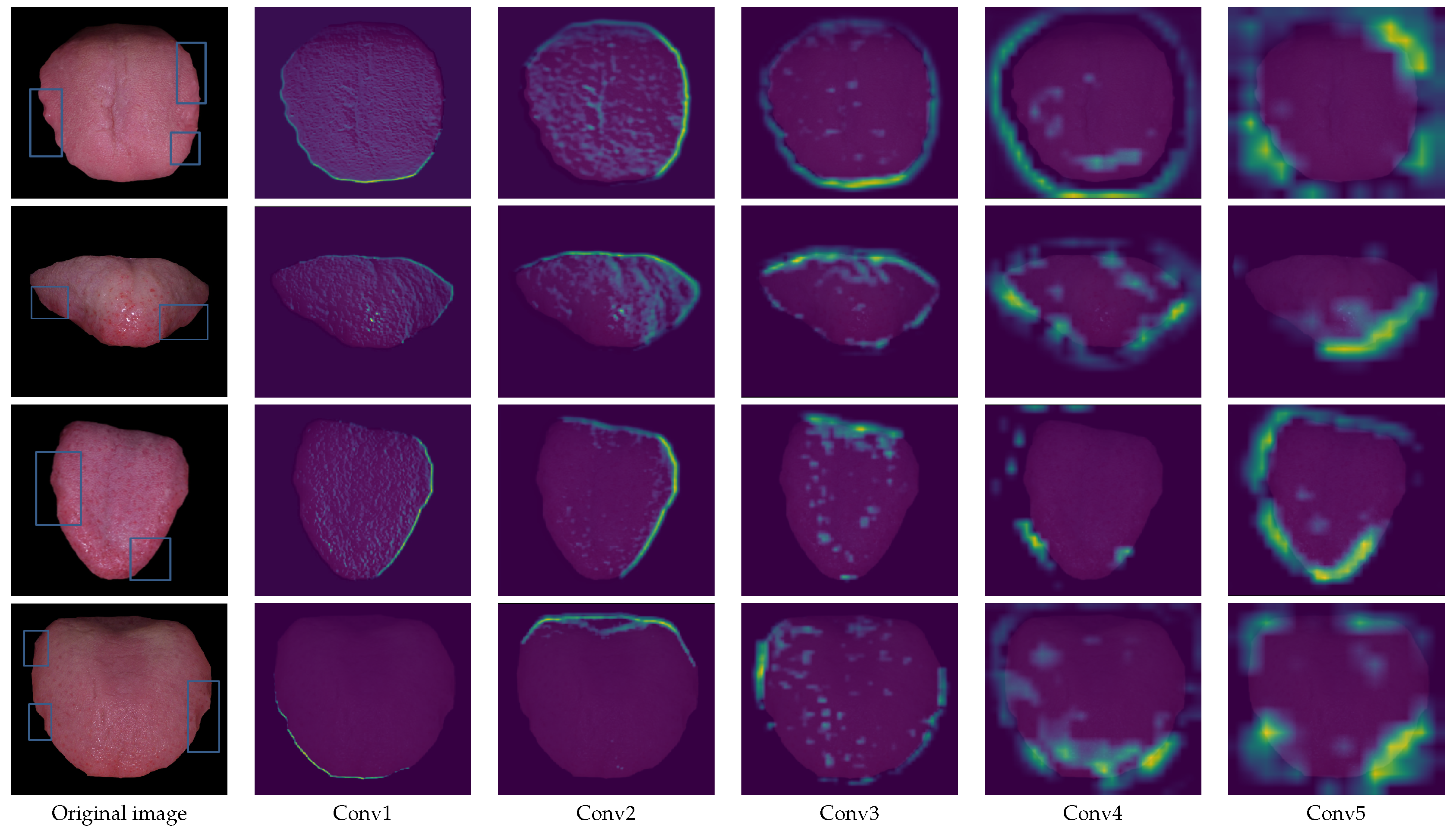
4.6. Model Interpretation
5. Conclusions
Author Contributions
Funding
Conflicts of Interest
References
- Shen, Z.Y. Basic theory of traditional Chinese medicine. Chin. J. Integr. Tradit. West. Med. 1997, 17, 643. [Google Scholar]
- Pang, B.; Zhang, D.; Wang, K. Tongue image analysis for appendicitis diagnosis. Inf. Sci. 2005, 175, 160–176. [Google Scholar] [CrossRef]
- McLean, N. Color atlas of oral diseases. Br. J. Plast. Surg. 2004, 100, 1299–1300. [Google Scholar] [CrossRef]
- Li, W.; Luo, J.; Hu, S.; Xu, J.; Zhang, Z. Towards the Objectification of Tongue Diagnosis: the Degree of Tooth-marked. In Proceedings of the IEEE International Symposium on It in Medicine and Education, Xiamen, China, 12–14 December 2008; pp. 592–595. [Google Scholar]
- Ren, Y.; Rong, L.; Ying, Z. Study on the correlation between dental scar tongue and constitution of traditional Chinese medicine in physical examination population. World Sci. Technol.-Mod. Tradit. Chin. Med. 2012, 14, 2283–2289. [Google Scholar]
- Li, X.; Yin, Z.; Cui, Q.; Yi, X.; Yi, Z. Tooth-Marked Tongue Recognition Using Multiple Instance Learning and CNN Features. IEEE Trans. Cybern. 2019, 49, 380–387. [Google Scholar] [CrossRef] [PubMed]
- Zhang, D.; Pang, B.; Li, N.; Wang, K.; Zhang, H. Computerized diagnosis from tongue appearance using quantitative feature classification. Am. J. Chin. Med. 2005, 33, 859–866. [Google Scholar] [CrossRef] [PubMed]
- Wang, Y.G.; Yang, J.; Zhou, Y.; Wang, Y.Z. Region partition and feature matching based color recognition of tongue image. Pattern Recognit. Lett. 2007, 28, 11–19. [Google Scholar] [CrossRef]
- Selvaraju, R.R.; Cogswell, M.; Das, A.; Vedantam, R.; Parikh, D.; Batra, D. Grad-CAM: Visual Explanations from Deep Networks via Gradient-Based Localization. In Proceedings of the International Conference on Computer Vision, Venice, Italy, 22–29 October 2017; pp. 618–626. [Google Scholar]
- Chiu, C.C. A novel approach based on computerized image analysis for traditional Chinese medical diagnosis of the tongue. Comput. Methods Progr. Biomed. 2000, 61, 77–89. [Google Scholar] [CrossRef]
- Pang, B.; Zhang, D.; Li, N.; Wang, K. Computerized tongue diagnosis based on Bayesian networks. IEEE Trans. Biomed. Eng. 2004, 51, 1803–1810. [Google Scholar] [CrossRef] [PubMed]
- Zuo, W.; Wang, K.; Zhang, D.; Zhang, H. Combination of polar edge detection and active contour model for automated tongue segmentation. In Proceedings of the International Conference on Image and Graphics, Hong Kong, China, 18–20 December 2004; pp. 270–273. [Google Scholar]
- Yu, S.; Yang, J.; Wang, Y.; Zhang, Y. Color Active Contour Models Based Tongue Segmentation in Traditional Chinese Medicine. In Proceedings of the International Conference on Bioinformatics and Biomedical Engineering, Wuhan, China, 6–8 July 2007; pp. 1065–1068. [Google Scholar]
- Wang, X.; Zhang, B.; Yang, Z.; Wang, H.; Zhang, D. Statistical analysis of tongue images for feature extraction and diagnostics. IEEE Trans. Image Process. 2013, 22, 5336–5347. [Google Scholar] [CrossRef] [PubMed]
- Huang, B.; Wu, J.; Zhang, D.; Li, N. Tongue shape classification by geometric features. Inf. Sci. 2010, 180, 312–324. [Google Scholar] [CrossRef]
- Zhang, Y. Research on Analysis Method of Tongue and Teeth-Marked Tongue. Ph.D. Thesis, Beijing University of Chinese Medicine, Beijing, China, 2005. [Google Scholar]
- Li, J.F.; Li, N.M.; Wang, K.Q.; Zhang, H.Z. Extracting feature of teeth-marked tongue image. In Proceedings of the Diagnosis Section of China Society of Integrated Traditional Chinese and Western Medicine, Fuzhou, China, 1 July 2009; pp. 100–105. [Google Scholar]
- Wang, H.; Zhang, X.; Cai, Y. Research on Teeth Marks Recognition in Tongue Image. In Proceedings of the Academic Conference on National Diagnosis of Chinese Society of Integrated Traditional Chinese and Western Medicine, Shenzhen, China, 30 May–1 June 2014; pp. 80–84. [Google Scholar]
- Shao, Q.; Li, X.; Fu, Z. Recognition of teeth-marked tongue based on gradient of concave region. In Proceedings of the International Conference on Audio, Language and Image Processing, Shanghai, China, 7–9 July 2015; pp. 968–972. [Google Scholar]
- Krizhevsky, A.; Sutskever, I.; Hinton, G.E. ImageNet classification with deep convolutional neural networks. In Proceedings of the International Conference on Neural Information Processing Systems, Lake Tahoe, NV, USA, 3–6 December 2012; pp. 1097–1105. [Google Scholar]
- Long, J.; Shelhamer, E.; Darrell, T. Fully convolutional networks for semantic segmentation. In Proceedings of the IEEE Conference on Computer Vision and Pattern Recognition, Boston, MA, USA, 7–12 June 2015; pp. 3431–3440. [Google Scholar]
- Zeiler, M.D.; Fergus, R. Visualizing and understanding convolutional networks. In European Conference on Computer Vision; Springer: Cham, Switzerland, 2014; pp. 818–833. [Google Scholar]
- Springenberg, J.T.; Dosovitskiy, A.; Brox, T.; Riedmiller, M. Striving for Simplicity: The All Convolutional Net. arXiv, 2014; arXiv:1412.6806. [Google Scholar]
- Zhou, B.; Khosla, A.; Lapedriza, A.; Oliva, A.; Torralba, A. Learning Deep Features for Discriminative Localization. In Proceedings of the Computer Vision and Pattern Recognition, Las Vegas, NV, USA, 27 June–30 June 2016; pp. 2921–2929. [Google Scholar]
- Mahendran, A.; Vedaldi, A. Understanding deep image representations by inverting them. In Proceedings of the IEEE Conference on Computer Vision and Pattern Recognition, Boston, MA, USA, 7–12 June 2015; pp. 5188–5196. [Google Scholar]
- Esteva, A.; Kuprel, B.; Novoa, R.A.; Ko, J.; Swetter, S.M.; Blau, H.M.; Thrun, S. Dermatologist-level classification of skin cancer with deep neural networks. Nature 2017, 542, 115–118. [Google Scholar] [CrossRef] [PubMed]
- Rajpurkar, P.; Irvin, J.; Zhu, K.; Yang, B.; Mehta, H.; Duan, T.; Ding, D.; Bagul, A.; Langlotz, C.P.; Shpanskaya, K.; et al. CheXNet: Radiologist-Level Pneumonia Detection on Chest X-Rays with Deep Learning. arXiv, 2017; arXiv:1711.05225. [Google Scholar]
- Mahendran, A.; Vedaldi, A. Visualizing Deep Convolutional Neural Networks Using Natural Pre-images. Int. J. Comput. Vis. 2016, 120, 233–255. [Google Scholar] [CrossRef]
- Kingma, D.; Ba, J. Adam: A Method for Stochastic Optimization. arXiv, 2014; arXiv:1412.6980. [Google Scholar]
- Girshick, R.B.; Donahue, J.; Darrell, T.; Malik, J. Rich Feature Hierarchies for Accurate Object Detection and Semantic Segmentation. In Proceedings of the Computer Vision and Pattern Recognition, Columbus, OH, USA, 23–28 June 2014; pp. 580–587. [Google Scholar]
- Simonyan, K.; Zisserman, A. Very Deep Convolutional Networks for Large-Scale Image Recognition. arXiv, 2015; arXiv:1409.1556. [Google Scholar]


| Accuracy | Precision | Recall | F1 Score | F2 Score | |
|---|---|---|---|---|---|
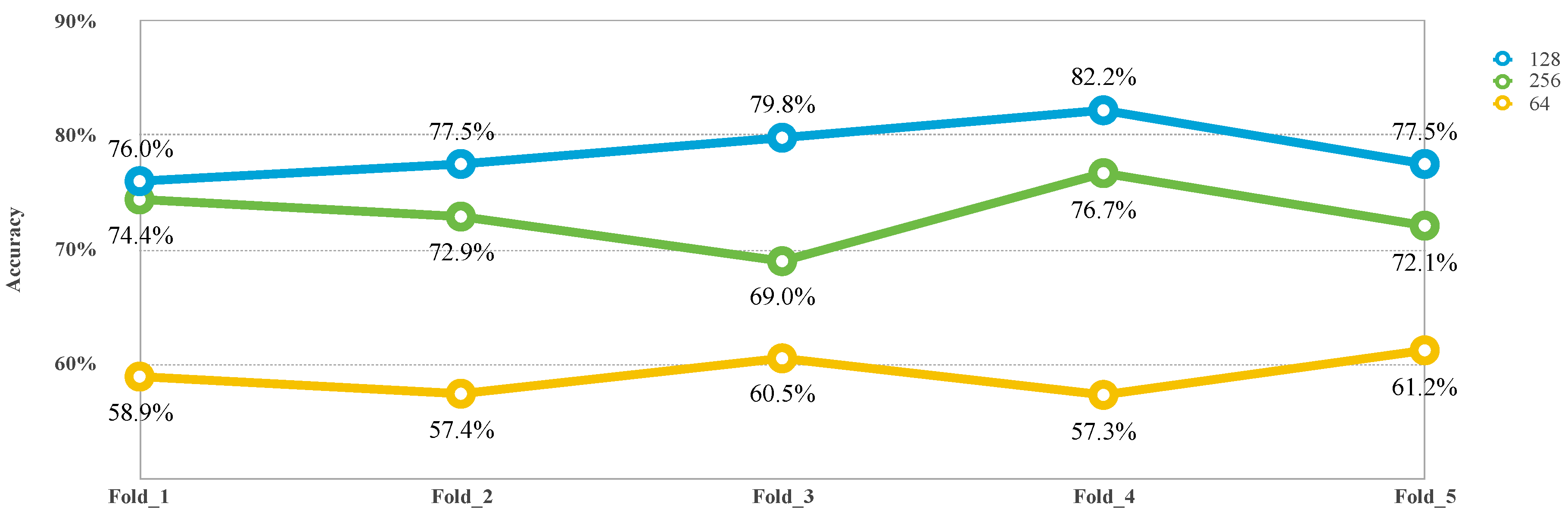
| Fold_1 | 76.0% | 74.2% | 73.8% | 0.74 | 0.74 |
| Fold_2 | 77.5% | 74.4%. | 75.6% | 0.75 | 0.76 |
| Fold_3 | 79.8% | 79.0% | 79.0% | 0.79 | 0.79 |
| Fold_4 | 82.2% | 84.1%. | 80.0% | 0.82 | 0.81 |
| Fold_5 | 77.5% | 70.7%. | 82.1% | 0.76 | 0.80 |
| Average | 78.6% | 76.5% | 78.1% | 0.77 | 0.78 |
| Kernel Size | Receptive Field | Accuracy | Precision | Recall | F1 Score | F2 Score |
|---|---|---|---|---|---|---|
| 3 × 3 | 94 | 78.6% | 75.9% | 78.1% | 0.77 | 0.78 |
| 5 × 5 | 156 | 76.0% | 74.1% | 74.1% | 0.74 | 0.74 |
| 7 × 7 | 218 | 73.6% | 71.1% | 72.9% | 0.72 | 0.73 |
| Conv Layer | Receptive Field | Accuracy | Precision | Recall | F1 Score | F2 Score |
|---|---|---|---|---|---|---|
| 3-Conv | 22 | 71.3% | 70.4%. | 62.1% | 0.66 | 0.64 |
| 4-Conv | 46 | 73.6% | 77.3%. | 56.1% | 0.65 | 0.59 |
| 5-Conv | 94 | 78.6% | 75.9% | 78.1% | 0.77 | 0.78 |
| 6-Conv | 190 | 72.1% | 72.5%. | 67.7% | 0.70 | 0.69 |
© 2019 by the authors. Licensee MDPI, Basel, Switzerland. This article is an open access article distributed under the terms and conditions of the Creative Commons Attribution (CC BY) license (http://creativecommons.org/licenses/by/4.0/).
Share and Cite
Sun, Y.; Dai, S.; Li, J.; Zhang, Y.; Li, X. Tooth-Marked Tongue Recognition Using Gradient-Weighted Class Activation Maps. Future Internet 2019, 11, 45. https://doi.org/10.3390/fi11020045
Sun Y, Dai S, Li J, Zhang Y, Li X. Tooth-Marked Tongue Recognition Using Gradient-Weighted Class Activation Maps. Future Internet. 2019; 11(2):45. https://doi.org/10.3390/fi11020045
Chicago/Turabian StyleSun, Yue, Songmin Dai, Jide Li, Yin Zhang, and Xiaoqiang Li. 2019. "Tooth-Marked Tongue Recognition Using Gradient-Weighted Class Activation Maps" Future Internet 11, no. 2: 45. https://doi.org/10.3390/fi11020045
APA StyleSun, Y., Dai, S., Li, J., Zhang, Y., & Li, X. (2019). Tooth-Marked Tongue Recognition Using Gradient-Weighted Class Activation Maps. Future Internet, 11(2), 45. https://doi.org/10.3390/fi11020045