Abstract
In this article, we work toward the answer to the question “is it worth processing a data stream on the device that collected it or should we send it somewhere else?”. As it is often the case in computer science, the response is “it depends”. To find out the cases where it is more profitable to stay in the device (which is part of the fog) or to go to a different one (for example, a device in the cloud), we propose two models that intend to help the user evaluate the cost of performing a certain computation on the fog or sending all the data to be handled by the cloud. In our generic mathematical model, the user can define a cost type (e.g., number of instructions, execution time, energy consumption) and plug in values to analyze test cases. As filters have a very important role in the future of the Internet of Things and can be implemented as lightweight programs capable of running on resource-constrained devices, this kind of procedure is the main focus of our study. Furthermore, our visual model guides the user in their decision by aiding the visualization of the proposed linear equations and their slope, which allows them to find if either fog or cloud computing is more profitable for their specific scenario. We validated our models by analyzing four benchmark instances (two applications using two different sets of parameters each) being executed on five datasets. We use execution time and energy consumption as the cost types for this investigation.
1. Introduction
Current prospects indicate that the number of devices connected to the Internet of Things (IoT) will reach the mark of 75 billion within the next decade [1], and this huge increase in scale will certainly bring new challenges with it. We can expect that when facing a scenario where several petabytes of data are produced every day, the massive volume of information will make transmitting it all to the cloud prohibitively costly in terms of time, money, and energy consumption. Thus, this outlook encourages us to examine current solutions and re-evaluate their potential in light of the new demands coming ahead.
As is often the case with big data, a possible way to meet these anticipated requirements is to not send every single byte to be processed by machines that are far from the data source, but instead bring the computation closer to where the information already is. Based on this concept, the recent paradigm called fog computing [2] was created and named after the idea that the fog can be seen as a cloud that is close to the ground. When working with fog computing, we can employ network edge devices (e.g., gateways, switches, and routers) and possibly the devices that are collecting data themselves to process the information.
Enabling computation to be performed near the data source has many advantages, such as allowing us to address issues related to transmission latency and network congestion. Moreover, it creates a window for new possibilities: filtering and discarding unnecessary information, analyzing readings in search of outliers that can be reported, combining readings from different sensors, and actual real-time response to local queries, among other applications. On the other hand, working with devices that are close to the edge of the network also means that we must handle IoT hardware with limited memory and processing power, energy consumption constraints, and new security, management, and standardization requirements [3].
With this trade-off in mind, we see that leveraging fog computing may become an appealing option for both academia and industry, as this would allow processes such as data analytics to benefit from working with more data. This could lead to data scientists not only being able to better understand the world we live in, but also making more accurate predictions and creating improved systems based on people’s behaviors and tastes.
However, even if fog computing is a very interesting choice in many situations, it is not the best solution in every possible case. For instance, if the computation that we are performing in the fog takes a long time to be completed when compared to the time that it takes for a value to be sent to the cloud, it might be more profitable to send the data to be processed by the more robust cloud servers instead of executing the program locally.
Considering this, we propose two models that aim at helping the user analyze the scenario that they are working with in order to decide whether fog or cloud computing is more profitable for them. The main contributions of this investigation are:
- A generic mathematical model that enables the calculation of fog and cloud computing costs based on a certain metric (e.g., number of instructions, execution time, energy consumed);
- A visual model that aids the comparison between fog and cloud costs and a threshold that defines which one should be chosen for a given set of parameters;
- A study of different approaches to estimate one of the parameters of the mathematical model and the impact of each approach on the performance of the test cases.
- An analysis of the proposed models using two different data filters as applications, with test cases for two distinct instances of each program being executed on five datasets (four containing real-wold data and one with artificial data). To this end, we consider the metrics execution time and energy consumption;
- A case study that explores how changing the parameters of our test cases would affect the decision between fog and cloud computing.
This article expands our previous work by presenting an investigation of different approaches to estimate one of the parameters of our mathematical model, as well as how this estimate affects performance; adding four real-world datasets to our tests; and including the analysis of energy consumption as a metric for our model. We now also discuss more studies related to ours in Section 2.
This text is organized as follows: Section 2 discusses other studies that also address system modeling. Section 3 presents our mathematical and visual models and describes how we can use them to choose between fog and cloud computing given a certain set of parameters. Section 4 has our test case analysis, where we investigate different approaches to estimating one of the parameters of the model, then go through the decision process with the help of our models, and finally simulate other values to study different scenarios. Lastly, Section 5 presents our conclusions and possibilities for future work.
2. Related Work
Mathematical models are an effective way to describe the behavior of systems and help users to better understand and optimize system performance. Therefore, many models have been proposed to estimate costs related to computing and transferring data. These costs, however, are dependent on the execution behavior of the task being considered and the highly-variable performance of the underlying resources. As such, remote execution systems must employ sophisticated prediction techniques that accurately guide computation offloading. These models are even more important for offloading systems, as they may need to decide whether or not it is worth sending a computation to other devices. To this end, many works have been proposed. However, they are usually complex, computationally expensive, or specific for some metric. We divided these works into general offloading schemes (Section 2.1) and fog-/cloud-aware schemes (Section 2.2).
2.1. Computation Offloading Schemes
Li, Wang, and Xu [4] considered offloading media encoding and compression computation from a small handheld device to a desktop via wireless LAN. They used profiling information from applications to construct cost graphs, which were then statically partitioned, and each part was set to run on either the small or the large device. The results showed considerable energy savings by offloading computation following that partition scheme. In another work [5], the authors tested the same infrastructure with benchmarks from the Mediabench suite using a Compaq iPAQ. Their scheme significantly saved energy in 13 of the 17 programs tested. Later, Li and Xu [6] considered the impact of adding security to the offload process for the same infrastructure. They added secure mechanisms such as SSL in all the offloaded wireless communication and concluded that despite the extra overhead, offloading remained quite effective as a method to reduce program execution time and energy consumption.
Kremer, Hicks, and Rehg [7] presented a prototype for an energy-aware compiler, which automatically generates client and server versions of the application. The client version runs on small devices, offloading computation to the server when necessary. The client also supports checkpoints to allow server progress monitoring and to recover from connection failures. They tested this compiler with multiple programs and mobile devices, measuring the energy consumption by actual power measurements, and showed that they could save up to one order of magnitude of energy in the small devices.
Rong and Pedram [8] built a stochastic model for a client-server system based on the theory of continuous-time Markovian decision processes and solved the offloaded dynamic-power management problem by using linear programming. Starting with the optimal solution constructed off-line, they proposed an online heuristic to update the policy based on the channel conditions and the server behavior, resulting in optimum energy consumption in the client and outperforming any existing heuristic proposed until the publication of their work by 35%.
Chen et al. [9] presented a framework that uses Java object serialization to allow the offloading of method execution as bytecode-to-native code compilation (just-in-time compilation). The framework takes into account communication, computation, and compilation energies to decide where to compile and execute a method (locally or remotely). As many of these variables vary based on external conditions, the decision is made dynamically as the methods are called. Finally, they tested the framework in a simulator and showed that the technique is very effective at conserving the energy of the mobile client.
O’Hara et al. [10] presented a system-wide model to characterize energy consumption in distributed robot systems’ computation and communication. With the model, they showed that it was possible to make better decisions of where to deploy each software and how to do the communication between robots. They tested this on a simulator and showed that for a search-and-rescue mission, there are several counterintuitive energy trade-offs, and by using their cost model scheme, AutoPower, they were able to improve by up to 57% over the baseline energy consumption.
Different from the others, Xian, Lu, and Li [11] chose to offload computation from one device to another by using a timeout approach instead of analyzing the software statically or dynamically. They set a specific amount of time in which the application would be allowed to run on the client and after a timeout, the program execution was entirely offloaded to the server. They showed that the heuristic works well and that it can save up to 17% more energy than approaches that tried to compute beforehand the execution time of the application.
Hong, Kumar, and Lu [12] showed a method to save energy in mobile systems that perform content-based image retrieval (CBIR). They proposed three offloading schemes for these applications (local search, remove extraction, and remote search) and physically measured that their approaches were able to save energy on an HP iPAQ hw6945 running CBIR applications.
Gu et al. [13] presented a dynamic partition scheme to decide when and which parts of a program to offload to nearby surrogates. They took into consideration both application execution patterns and resources fluctuations to use a fuzzy control policy model. They ran an extensive number of tests, measuring the total overhead, the average interaction delay (time to send and receive requested data), and the total bandwidth required. The results showed that their model was effective as an offloading inference engine.
Gurun, Krintz, and Wolski [14] argued that offloading systems must predict the cost of execution both locally and remotely. Moreover, these techniques must be efficient, i.e., they cannot consume significant resources, e.g., energy, execution time, etc., since they are performed on the mobile device. Thus, the authors proposed NWSLite, a predictor of resource consumption for mobile devices. They empirically analyzed and compared both the prediction accuracy and the cost of NWSLite and a number of different forecasting methods from existing remote execution systems, showing its advantages over the other systems.
Wang and Li [15] used parametric analysis to deal with the issue of programs having different execution behaviors for different input instances. They proposed a cost analysis for computation and communication of a program that generates a function of the program’s inputs. With this approach, better decisions can be made when partitioning a program and making offload decisions based on the program input.
Wolski et al. [16] proposed a method to make offloading decisions in grid settings by using statistical methods. When only considering the network bandwidth of the system, they showed that a Bayesian approach can be superior to prior methods.
Nimmagadda et al. [17] showed that offloading mechanisms can even be feasible in real-time scenarios such as real-time moving object recognition and tracking. They considered the real-time constraints when building the offloading decision system and tested motion detection and object recognition using offloading in multiple network and server configurations.
2.2. Fog/Cloud Aware
Jayaraman et al. [18] presented equations for a cost model that focuses on energy usage and evaluates the energy gain of their approach when compared to sending all the raw data to the cloud. They also introduced the CARDAP platform, which was implemented for Android devices with the aim of distributing mobile analytics applications in an energy efficient way among mobile devices in the fog.
Deng et al. [19] investigated the trade-off between power consumption and transmission delay in fog-cloud computing systems. Their model was formulated as a workload allocation problem where the optimal workload allocations between fog and cloud intended to minimize power consumption given a constrained service delay. Their aim was to provide guidance to other researchers studying the interaction and cooperation between the fog and cloud.
Xu and Ren [20] analyzed an edge system consisting of a base station and a set of edge servers that depend on renewable power sources. Their models considered workload, power, battery, and delay cost, and they used them to formulate the dynamic offloading and autoscaling problem as an online learning problem in order to minimize the system cost.
Liu et al. [21] used queuing theory to study a mobile fog computing system. Their model was formulated as a multi-objective optimization problem with a joint objective to minimize energy consumption, execution delay, and payment cost by finding the optimal offloading probability and transmission power for each mobile device. They addressed the multi-objective optimization problem with an interior point method-based algorithm.
2.3. Our Approach
This article presents a general mathematical model and a visual model created to assist the analysis of the fog-cloud computing cost trade-off. Therefore, we note that our main goal is different from that of other mentioned works, given that we intend to enable users to select the most profitable platform according to a metric of their choosing, while the other studies focus on optimizing specific metrics (mostly time and energy). Another example of a visual approach is the roofline model introduced by Williams, Waterman, and Patterson [22], which served as inspiration for our model.
Furthermore, the presented model is simple enough such that its implementation can run on resource-constrained devices, which is not the case for most of the models listed in this section. Although some approaches such as NWSLite [14] also discuss the cost model needing to be small and constrained, it is still far more complex than our approach and far too large to be used in the constrained devices with which we work. We consider this to be a relevant distinction, as constrained devices will have a growing importance in the Internet of Things due to having low power consumption and reduced cost, size, and weight.
3. Modeling Platforms
When working with sensors, it is common for users to need to transform the raw collected data into something else before storing the final values. For example, they may wish to standardize or clean the data (parsing), discard unwanted readings (filtering), or generate knowledge (predicting).
With the task at hand, they will then need to decide where to execute it, and there are a few options to choose from: they can process the data on the same device that collected the values; they can send the data to other nearby devices, among which the task may be split; or they can send the data to be processed by more powerful and distant devices, such as cloud data centers.
In this article, we discuss the first and third cases, with the second one being left to future work. Therefore, our main goal will be working toward the answer to the question “is it worth processing a data stream on the device that collected it or should we send it somewhere else?”. In a way, looking for the answer to this question is akin to a search for cases where fog computing (performing computation close to the data source) is more profitable than cloud computing (sending data to be processed by faraway devices).
For the purpose of this analysis, we consider that we are working with devices that are capable of executing custom code, connected to the Internet, and able to send packets to other devices. Furthermore, we assume that we are handling non-empty data streams with a limited size (i.e., the stream size is neither zero, nor infinite).
3.1. General Equations
First, we look at the cost of performing the task on the device itself, which we call fog computing cost (). We model this cost with regard to the steps that must be executed to complete the computation. We start by reading the sensor value (cost r). Then, we perform a custom code operation (cost t). We are particularly interested in filtering procedures, as these can be simple enough to run on resource-constrained devices [23] and have the potential to decrease the amount of data sent to the cloud drastically, a situation that is posed to become a problem with the large-scale adoption of technologies such as the Internet of Things. For that reason, in this investigation, we consider that our custom operations are filters, that is, operations that decide whether or not each stream value should be sent to the cloud. In this case, we must also consider the cost of sending the data to the cloud (s) and the probability that the value will pass the filter in question (f). After completing the operation, the device is then idle until a new reading comes along (cost i). If we are working with a data stream of size z, Equation (1) shows the fog computing cost. We are only dealing with cases where there is no overlap between processing and transferring the data, and accounting for this approach will be a future extension of our model.
Next, we look at the cost of performing the task in the cloud. As some of the resources used by the cloud are not under the user’s control, from the point of view of the device that is collecting the data, the cloud computing cost () only includes, for each of the z values in the data stream, reading (r), sending (s), and being idle (i), as shown by Equation (2).
Given that these are generic models, it is possible to plug in values to calculate different types of costs (e.g., number of instructions, execution time, energy consumed). We will use this approach in Section 4 to analyze a few test cases. We note that we are considering that all of the values are positive, with the exception of f, which is a probability and, as a result, a number between zero and one. Table A1 in Appendix A has a summary of the notation introduced in this subsection.
In order to answer our question, we would like to choose situations where the fog computing cost is less than or equal to the cloud computing cost (we use the fact that processing data locally decreases network traffic congestion as a tiebreaker in favor of fog computing when fog and cloud costs are the same). Thus, in the cases where , we have:
Since f is the probability of a value passing the filter, is the probability of a value being filtered out. Therefore, from Equation (3), we have that the probability that a value will be filtered must be greater than or equal to for us to choose fog computing in this cost model.
3.2. Estimating f
We can find s and t by measuring the hardware and software infrastructures according to the type of cost for which we are looking. However, f also depends on the data, so it cannot be as easily calculated unless we know all data points in advance. What we can do instead is estimate f by looking at a subset of the values.
We can start by plotting a graph to guide our analysis of the relationship between and . In this graph, the horizontal axis represents the fog computing cost as a function of the number of stream values being processed in the fog. Therefore, a case where all z data points are processed in the fog would be represented by a point crossing this axis. The value of this point, which we call , can be calculated by Equation (1). In the same way, the vertical axis represents the cloud computing cost from the point of view of the device as a function of the number of stream values being processed in the cloud, and a case where all values are handled by the cloud is represented by a point crossing this axis. The value of this point, which we call , can be found with the help of Equation (2).
We can also add more points to the graph by considering the cases where part of the data is processed by the fog, while the rest is processed by the cloud. For each additional sensor reading that we process in the fog instead of just sending to the cloud, we add to the value in the horizontal axis and subtract from the value in the vertical axis. It is possible to repeat this process until all possibilities are represented in the graph.
Lastly, we draw a line that passes through these points, which will give us the linear equation represented in Equation (4).
Figure 1 shows an example of a graph constructed with the method described in this section. In this graph, and all the lines have the same values for all variables, except f.
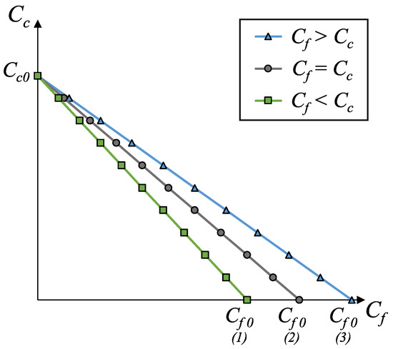
Figure 1.
Graph of the relationship between fog and cloud computing costs.
Considering that we are estimating f on the device itself while it is collecting and processing the data, we do not need to worry about situations where , as the values are processed on the device before we make our decision and nothing will change if fog computing is considered to be more profitable. To evaluate the scenario where , we can think about the worst-case scenario of (i.e., all data are passing the filter) and determine the size of the penalty that we are willing to pay to be able to make a more informed decision about the value of f. First, we calculate the penalty (p) of processing each additional value on the fog when it would be more profitable to do so on the cloud using Equation (5). This value is a percentage of increase in cost.
As , , and thus, p is always positive. Then, we can establish a threshold for the maximum penalty that we are willing to pay. For example, if , each additional point processed in the fog will increase the computational cost by . Therefore, if we are willing to risk up to a increase in cost, we can test if the first data points pass the filter or not. In this case, if out of the five values pass the filter, we can estimate that and then plug this value into Equation (3) to make our decision. It is up to the user to define what is a reasonable trade-off given the parameters of their specific scenario. Table A1 in Appendix A has a summary of the notation introduced in this subsection.
Examining Equation (4) and Figure 1 also gives us additional insights when we evaluate the slope of the line, which is . When , the slope is (as is the case of the gray line with circular markers). If , the slope is less than (green line with square markers), and for , it is greater than (blue line with triangular markers). From that, we have the following:
Considering that all values are positive (or possibly zero in the case of f), we can follow a similar logic for the cases where and . We see that Equation (6) is analogous to Equation (3), but in this case, it helps us notice that the values of r, i, and z do not affect the comparison between the slope and . Therefore, we can look only at the values of f, s, and t when deciding whether to perform the computation on the fog or the cloud using our cost model. We will use this simplification for our analysis in Section 4.
4. Analyzing Test Cases
We will now put our theory to practice by applying it to some test cases used in previous studies [23,24]. Namely, the MinMax and Outlier benchmarks. MinMax is a simple filter, which only allows numbers outside of a certain range to pass, and Outlier is a procedure that executes Tukey’s test [25] to detect outliers in a window of values. We chose four instances of the benchmarks: MinMax , which filters out numbers in the range; MinMax , the same program, but using the range instead; Outlier 16, which finds outliers in a window of 16 values; and Outlier 256, the same program, but with a window of 256 values instead. The parameters of each benchmark were selected due to previous work that showed that these four instances filter out very different percentages of stream values [23].
We executed these benchmarks for five different datasets: four real-world datasets downloaded from the United States National Oceanic and Atmospheric Administration’s National Centers for Environmental Information website [26] and an artificial dataset, which represents a stream of sensor readings [23]. The four real datasets are a subset of the hourly local climatological data collected at Chicago O’Hare International Airport between September 2008 and August 2018 and are named HOURLYRelativeHumidity (HRelHumidity, the relative humidity given to the nearest whole percentage, with values between 16 and 100), HOURLYVISIBILITY (HVisibility, the horizontal distance an object can be seen and identified given in whole miles, with values between 0 and 10), HOURLYWETBULBTEMPC (HWBTempC, the wet-bulb temperature given in tenths of a degree Celsius, with values between −27.3 and 27.4), and HOURLYWindSpeed (HWindSpeed, the speed of the wind at the time of observation given in miles per hour, with values between 0 and 55). We call the artificial dataset Synthetic, and its values are random floating-point numbers between −84.05 and 85.07. These values were generated by using the sine function combined with a Gaussian error.
In our tests, we used the stream size z = 65,536, which is one of the stream sizes analyzed in previous work [23], while also being a reasonably large stream size for which our test cases can be executed in a feasible time.
As we have the infrastructure to measure the execution time of our benchmarks on a NodeMCU device [23], we used time as one of the cost types for this analysis. The other cost type is energy consumption, which we obtained in two different ways: the first way was by combining the NodeMCU execution times with electric current and voltage information to calculate the energy consumption of executing the benchmarks on this device; the second way was to use the number of instructions, host per guest instruction, and average cycles per instruction combined with electric current, voltage, and clock rate information to calculate the energy consumption of executing the benchmarks on other devices, such as a Raspberry Pi 3. Section 4.3 has a more detailed explanation of these two approaches.
For the results reported in this article, we used the execution time and energy consumption values as the input for simulations that calculate the fog and cloud computing costs according to our model, but we intend to implement a system that uses our model to choose between processing values in the fog or the cloud as future work.
We divided our analysis into four parts. As we need the value of f in order to calculate the fog computing cost, Section 4.1 investigates different ways to implement the estimation approach described in Section 3.2. Section 4.2 then uses the result of the previous subsection to calculate the fog and cloud computing costs using execution time as the cost type. Similarly, Section 4.3 presents the costs regarding energy consumption. These two subsections evaluate the efficiency of the chosen estimation technique and how well our model employs it to choose between processing values in the fog or in the cloud. Finally, Section 4.4 describes a way to use our model to simulate different scenarios, allowing us to observe how changing the values of our parameters would affect the decision between fog and cloud.
4.1. Choosing an Approach to Estimate f
When following the steps presented in Section 3.2 to estimate the probability that a value passes the filter (f), we come across the question of whether it would be more profitable to make a decision at the beginning of the stream and then process the values accordingly or to make several decisions along the stream with the intent of accounting for possible changes in data patterns.
In order to evaluate the possibility of making several decisions along the stream, we implemented two different estimation procedures, which we call Local and Cumulative. In both approaches, we first divide our stream into a certain number of blocks (b). As the number of values we are allowed to test (v) is still the same, we can now check values in the first blocks and values in the last block. The total number of elements in each block depends on the stream size (z) and can be calculated as for the first blocks and for the last one.
In the Local approach, we leverage the information obtained by testing local values in order to try to better estimate f for each block. To that end, we test the values at the beginning of each block and count how many of them passed the filter, then divide this number by the number of tested values. Continuing the example from Section 3.2, for , we would be able to check data point in each of the first three blocks and data points in the last one. If the number of values that passed the filter (n) was one in each of the first and second blocks, none passed the filter in the third, and one passed it in the fourth, we would have , , , and for each block, respectively.
In the Cumulative approach, we attempt to use the results from all previously-tested blocks in order to make a more informed estimate using a larger number of data points. In this case, we also test the values at the beginning of each block and count how many passed the filter, but we then accumulate the number of both tested and passed values with the count from previous blocks. In our example, that would lead to for the first block, for the second block, for the third, and for last block.
Using these two approaches to estimate f, we calculated the costs in terms of execution time for all benchmarks and datasets using the simplified versions of Equations (1) and (2) obtained in Section 3.2 (i.e., and ). The figures in this subsection present a summary of these results. For the sake of simplicity, we did not include all possible combinations between datasets and applications, as some of the graphs are very similar to the ones shown. All figures employ the same values for stream size (z = 65,536) and custom execution code cost (t, shown in Table A2 and Table A3 in Appendix B), but Figure 2, Figure 3, Figure 4 and Figure 5 use the measured time of [24] as the cost of sending data to the cloud (s), while Figure 6, Figure 7, Figure 8 and Figure 9 show what the costs would be like if s was ten times smaller ( ). In the first case, the results are fog-prone, that is, the fog is more likely to be profitable, as s is about one order of magnitude larger than t. On the other hand, the results in the second case are cloud-prone, as the cloud is more likely to be profitable when we have close values for s and t.
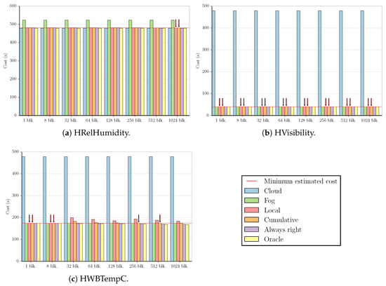
Figure 2.
Summary of the results for MinMax fog-prone test cases. Blk., block(s).
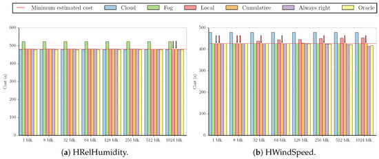
Figure 3.
Summary of the results for MinMax fog-prone test cases.
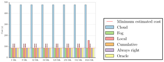
Figure 4.
Summary of the results for Outlier 16 fog-prone test cases (HVisibility).
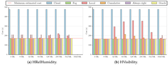
Figure 5.
Summary of the results for Outlier 256 fog-prone test cases.
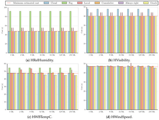
Figure 6.
Summary of the results for MinMax cloud-prone test cases.
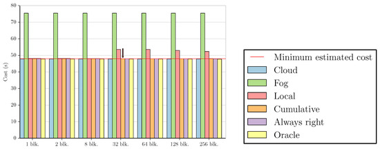
Figure 7.
Summary of the results for MinMax cloud-prone test cases (HWBTempC).
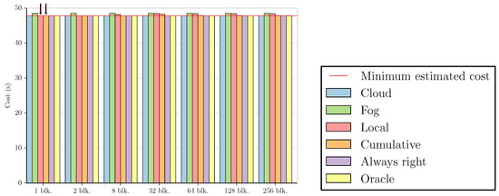
Figure 8.
Summary of the results for Outlier 16 cloud-prone test cases (HWBTempC).
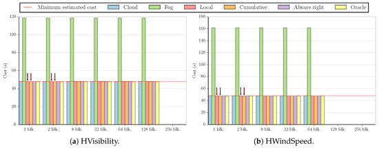
Figure 9.
Summary of the results for Outlier 256 cloud-prone test cases.
These figures compare the cost of processing all data in the cloud (Cloud); processing all data in the fog (Fog); the cost of using the Local and Cumulative approaches to estimate f and then decide where the data should be processed in each block (Local and Cumulative, respectively); what the cost would be if there was a procedure that always chose correctly between the fog and the cloud after testing the values at the beginning of each block (Always right); and what the cost would be if we knew where to process the data in each block without any testing (Oracle). The red line in each graph shows the minimum estimated cost among all the tested numbers of blocks for a certain combination of dataset and benchmark, considering only Local and Cumulative estimates. The red arrows point to all Local and Cumulative bars that have the same value as the minimum cost.
We start by analyzing the fog-prone results. The graphs for the MinMax benchmark present three different sets of characteristics. The first can be seen in Figure 2a. Despite being fog-prone, the most profitable choice in this case is the cloud. The division into 1024 blocks gives us the best estimate, increasing the cost by in comparison to sending all values to the cloud. However, we note that the estimate obtained by using one block increases the cost by only .
The second case is the one shown in Figure 2b, which is similar to the results for the HWindSpeed and Synthetic datasets (the difference being that the cost values are around 100 and 300 for these two datasets, respectively). Here, all the divisions result in the same estimate for both the Local and Cumulative approaches. For HWindSpeed and Synthetic datasets, the Cumulative approach results in the same estimate for all values, with Local starting to have increasingly worse estimates with 256 blocks and 512 blocks, respectively.
The third case is the one depicted in Figure 2c. Although the Cumulative approach shows good estimates for a higher number of blocks, we see that both Local and Cumulative obtain the minimum cost value for one and eight blocks, as well.
The graphs for MinMax show two sets of characteristics. Figure 3a illustrates the first one, which is a similar result to that of Figure 2a, and Figure 3b depicts the second, which is akin to the graphs for the HVisibility, HWBTempC, and Synthetic benchmarks. In this case, dividing the stream into only one block results in the minimum cost value for all benchmarks except HWBTempC, for which the Cumulative approach reduces the cloud cost by when dividing by 128 blocks, compared to for just one block.
All graphs for the Outlier 16 benchmark are similar to Figure 4, with every estimate resulting in the minimum cost apart from the Local approach using 1024 blocks (for the Synthetic benchmark, even this case results in the minimum cost).
For Outlier 256, most graphs look like Figure 5a, where dividing by up to 32 blocks in both approaches results in the minimum cost. Unlike the other datasets, HVisibility allows us to test the division by 1024 blocks, as seen in Figure 5b, given that the number of values we can test in this case is larger than 1024, and therefore there is at least one value per block.
Analyzing these results, we observe that in most cases, changing the number of blocks or the estimation procedure only affects the costs by a slight margin, with the difference between the fog and cloud computing costs being much more prominent.
We now look at the cloud-prone results. Figure 6a has the results for the MinMax benchmark running on the HRelHumidity dataset. All estimates result in the minimum cost, which is an increase of over the cost of processing all data in the cloud.
While the results shown in Figure 6b are cloud-prone, we see that in fact, the fog is more profitable when executing the MinMax benchmark on the HVisibility dataset, with all estimates having approximately the same cost as processing all values in the fog (less than a difference).
Figure 6c also shows one of the datasets for the MinMax benchmark, HWBTempC. This result is somewhat similar to that of the Synthetic dataset in the sense that the cloud is more profitable in both cases; the Local approach presents a few estimates with high cost (with two and eight blocks for HWBTempC and with 128 and 256 blocks for Synthetic), and only one estimate has the lowest cost value (Local with 256 blocks for HWBTempC and Cumulative with 64 blocks for Synthetic).
Figure 6d displays the final dataset for the MinMax benchmark. Similar to Figure 6b, this test also presents a lower cost for processing all data in the fog. However, the difference between cloud and fog costs is much smaller in this case, and the best estimate (Local with 64 blocks) reduces the cost of processing all data in the fog by .
Figure 7 illustrates the results for MinMax , which are similar for all datasets. In this benchmark, processing all the data in the cloud costs much less than doing so in the fog, and the Local approach usually yields higher estimates for several block numbers (with the exception of HRelHumidity, where all estimates are the same in both approaches). Using only one block results in the minimum cost for the HRelHumidity and HWindSpeed datasets, but the difference in cost of using only one block when compared to the minimum cost in the other datasets is only , , and for HVisibility, HWBTempC, and Synthetic, respectively.
As we can see in Figure 8, the values for the cost of processing all data in the cloud and in the fog are very similar for Outlier 16. This is the case for all datasets in this benchmark, but the minimum value is achieved by different numbers of blocks in distinct datasets. For HRelHumidity and HWBTempC, the minimum is obtained by using one block; for HWindSpeed, two; for Synthetic, eight; and for HVisibility, 256. Both Local and Cumulative approaches present the same results for the minimum cost case in all datasets except HVisibility, where the Local approach presents a lower cost.
Similarly to Figure 5a,b, most of the graphs for the Outlier 256 benchmark apart from the dataset HVisibility (Figure 9a) look like the one in Figure 9b. Again, this is due to the fact that only the HVisibility dataset allows us to test at least one value per block, in this case for 128 blocks. In all cases, dividing by one or two blocks results in the minimum cost for both the Local and Cumulative approaches. For HWBTempC, dividing by eight blocks also yields this result.
Again, we can see that in most cases, changing the number of blocks or the estimation procedure does not have a large impact on the cost, and simply choosing correctly between the fog and the cloud will lead to most of the performance gains.
Therefore, this evaluation allows us to conclude that using the straightforward solution of looking at the first values of the stream (that is, when there is only one block) leads to good results in terms of cost for several test cases. Furthermore, in the instances where this is not the best approach, the increase in cost is very small, not justifying the use of more complex division methods. Considering this, in the following subsections, we will look at the values at the beginning of the stream to estimate f.
4.2. Deciding between Fog and Cloud Considering Execution Time
As seen in Section 3, we only depend on the variables s, t, and f for our calculations, so we start by finding these values. Table A2 and Table A3 in Appendix B show the values for t in milliseconds measured for each benchmark and dataset, and we use the measurement of [24] in all fog-prone test cases and for the cloud-prone ones. Having these values, we can now calculate and for the worst-case scenario from the fog point of view, that is, when .
We are considering that z = 65,536, so we can use Equation (5) to determine the penalty for processing a value in the fog when it would cost less to do so in the cloud (p). Given our large stream size, the penalty for each value is very small in fog-prone cases (less than ) and still relatively small in cloud-prone ones (less than ), as can be seen in Table A2 and Table A3 in Appendix B. This difference is due to the fact that values for s and t are closer to each other in our cloud-prone cases.
Therefore, we can look at a reasonable number of values and still have a very low increase in cost. We decided that we are willing to have a maximum increase in cost of , so that enables us to test over 3000 values for Outlier 16 and both MinMax cases, over 900 values for Outlier 256 for fog-prone cases, and ten times fewer values for cloud-prone cases (the exact numbers are also displayed in the aforementioned table). By examining the output of the benchmarks, we are able to count the values that passed the filter (n), which leads us to the f estimates, as well as the real f values for comparison. Again, all of these results are reported in Table A2 and Table A3.
Finally, we use the calculated f values to plot a graph similar to the one in Figure 1 for each benchmark. Like Section 4.1, here, we also used the simplified versions of Equations (1) and (2) (i.e., and ). The result is illustrated in Figure 10. The continuous lines represent the tests that use the estimated values of f (Est.), and the dashed lines represent the tests that use the real values of f (Real). The continuous thick gray line represents the case where , that is, a line with a slope of . By observing the graphs, we can determine that most of the lines are below the threshold for fog-prone cases and above it for cloud-prone cases, as expected. As discussed in Section 3, the lines below the threshold mean that it is more profitable in terms of execution time to run these filters in the device that is collecting the data instead of sending the values to be processed in the cloud. On the other hand, lines above the threshold mean that, from the point of view of the device, it is more profitable to process these data on the cloud.
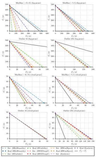
Figure 10.
Graphs of the linear equations for each dataset and benchmark using execution time as the cost. Est., estimated.
A few notable exceptions are the MinMax benchmarks being executed on the HRelHumidity dataset in the fog-prone scenario and the MinMax benchmark being executed on the HVisibility and HWindSpeed datasets on the cloud-prone scenario. In the first case, we see that although it was more likely that the fog would be more profitable, the lines are above the threshold, indicating that in fact the cloud is the correct choice. This can be explained by looking at the values of f for the MinMax benchmarks on the HRelHumidity dataset, which are equal to one, meaning that all values passed the filter. We can see that the cloud is more profitable every time this happens, as is always larger than . In the second case, the lines are below the threshold, indicating that the fog is more profitable instead of the cloud. This can again be explained by looking at the values of f. MinMax has for HVisibility and for HWindSpeed. Using the values of s and t in each case, we can calculate what f would be when . For HVisibility, , leading to . For HWindSpeed, and . The f value for both test cases is below the f value for the threshold, indicating that the fog is indeed the correct choice for them.
We can also calculate the values of the slopes in order to verify the accuracy of our f estimation. We do so by determining the slope of each of the lines using both the estimated and real f values. The slopes obtained, as well as the error of the estimated values in comparison to the real ones, are shown in Table A2 and Table A3 in Appendix B. In 16 out of the 20 fog-prone cases and in 16 out of the 20 cloud-prone cases, the error is less than in our predictions, which we consider a good result, as we are able to get a close estimate of f while only risking an increase of in the processing cost. Furthermore, it is worth noting that while the eight remaining test cases present larger errors, the choice between fog and cloud is the correct one in all of them.
4.3. Deciding between Fog and Cloud Considering Energy Consumption
Similarly to what we did in the previous subsection, we start by obtaining values for s, t, and f. However, we will now use energy consumption as our cost type and evaluate our test cases on two different devices, namely a NodeMCU platform and a Raspberry Pi 3 board.
For the NodeMCU, we calculate t by taking the execution time for each test case (displayed in Table A2 and Table A3 in Appendix B) and multiplying it by the voltage of the device (2 ) and the electric current for when no data are being transmitted ( ) [27], resulting in the values reported in Table A4 and Table A5 in Appendix B. We use the same method to calculate the values of s, multiplying the time it takes to send the data to the cloud ( for fog-prone cases and for cloud-prone cases) by the voltage and by the electric current for when data are being transmitted (70 ) [27], producing for fog-prone cases and for cloud-prone ones. The next step is to calculate and for , the worst-case scenario from the fog point of view.
Given z = 65,536, we use Equation (5) to determine the penalty for processing a value in the fog when it would cost less to do so in the cloud (p). Table A4 and Table A5 have all the values for p, which are less than 0.0002 for fog-prone scenarios and less than 0.006 for cloud-prone scenarios. We again use as the limit for the increase in cost that we are willing to pay to estimate the value of f, which allows us to test over 13,000 values for most fog-prone cases (with the exception of Outlier 256, where v ranges between 3600 and 5700, as this benchmark executes a more costly procedure in comparison to the others) and over 320 values for most cloud-prone ones (here, the values of v range between 90 and 150 for Outlier 256), as can been seen in Table A4 and Table A5.
The last step is to estimate f and plot the resulting linear equations using the simplified versions of Equations (1) and (2) (i.e., and ), as illustrated by Figure 11. From Table A4 and Table A5, we see that the slope estimate error is less than in 13 out of the 20 fog-prone cases and in 16 out of the 20 cloud-prone ones, which again is a good result for only maximum risk in the processing cost. Moreover, from the 11 remaining test cases, 10 correctly choose the more profitable approach (the case that does not choose correctly is discussed below). We see that these results are analogous to the ones obtained in Section 4.2, with the expected choice being made on most fog- and cloud-prone cases and the same four test cases appearing as exceptions (fog-prone MinMax and MinMax executed on HRelHumidity and cloud-prone MinMax on HVisibility and HWindSpeed).
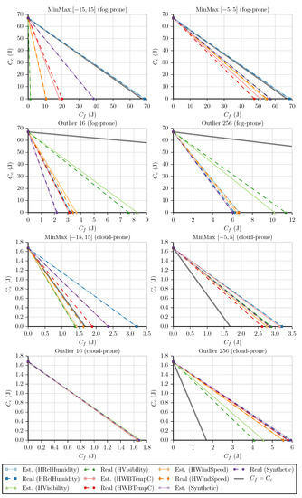
Figure 11.
Graphs of the linear equations for each dataset and benchmark using energy consumption as the cost: NodeMCU.
Nonetheless, we can see one interesting difference in the cloud-prone Outlier 16 cases, as all lines are very close to . In this type of situation, it is necessary to check the slope values to get a more accurate view of the decisions being made. From Table A5, we have the following slope estimates (and real values): for HRelHumidity, −1.0070 (−1.0128); for HVisibility, −0.9836 (−1.0105); for HWBTempC, −1.0106 (−1.0032); for HWindSpeed, −1.0019 (−1.0048); and for Synthetic, −0.9990 (−0.9945). From that, we have that fog is chosen for HRelHumidity, HWBTempC, and HWindSpeed, with the cloud being chosen for the other two datasets. However, in the case of HVisibility, the real slope value tells us that the best choice would have been processing the values on the fog. Even so, considering how close the fog cost ( ) is to the cloud cost ( ) in this case, choosing the less profitable option will not greatly affect the performance of the system.
Instead of also executing our test cases on a Raspberry Pi 3 device, we employ a different approach to calculate the value of t. First, we use our infrastructure [23] to count the number of instructions for each test case (displayed in Table A6 and Table A7 in Appendix B). As our infrastructure is a virtual machine, we then multiply this number by the number of host per guest instructions (60 for MinMax and 66 for Outlier [23]) and by the average number of cycles per instruction (which we estimate to be one). This gives us an estimate of the number of cycles that each test case would take to process the whole data stream on the Raspberry Pi 3. We then divide this result by the clock rate ( [28]) to find out the time each test case takes to process all stream values and by the stream size (z = 56,536) to finally obtain the execution time of each test case. We then proceed with the same method that we used for NodeMCU to obtain the t values reported in Table A6 and Table A7. In this device, the voltage is , and the electric current for when no data are being transmitted is 330 .
We determine the value of s in the same way as we did for NodeMCU, that is, by multiplying the time it takes to send the data to the cloud ( for fog-prone cases and for cloud-prone cases) by the voltage and by the electric current for when data are being transmitted (500 ) [28], which gives us for fog-prone cases and for cloud-prone ones.
After that, we calculate and for and use Equation (5) to determine the penalty for processing a value in the fog when it would cost less to do so in the cloud (p, which can be found in Table A6 and Table A7). In the fog-prone cases, p is less than 0.00001, and in the cloud-prone cases, it is less than 0.03. This time, we use as the limit for the increase in cost that we are willing to pay to estimate the value of f in the fog-prone cases and as the limit in cloud-prone cases. This is done due to the fact that we have very small values for p in the former and larger values for p in the latter. With these limits, we can test over 11,000 values for most fog-prone cases (with the exception of Outlier 256, where v ranges between 1700 and 2900) and over 290 values for most cloud-prone ones (here, the values of v range between 40 and 80 for Outlier 256), as indicated in Table A6 and Table A7.
Finally, we estimate f using the simplified versions of Equations (1) and (2) to plot the graphs in Figure 12. Table A6 and Table A7 show us that 10 out of the 20 fog-prone cases and 16 out of the 20 cloud-prone ones have a slope estimate error of less than . Although there are four fog-prone scenarios where the error is higher than and three cloud-prone scenarios where it is higher than , the most profitable option between cloud and fog is chosen in all cases.
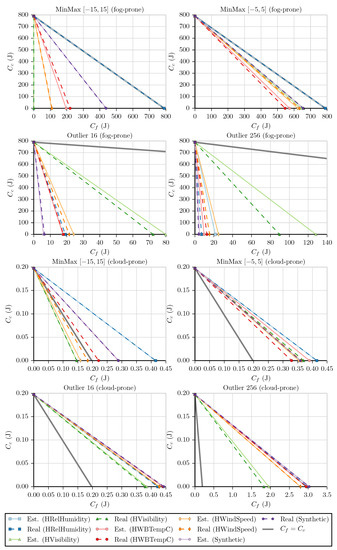
Figure 12.
Graphs of the linear equations for each dataset and benchmark using energy consumption as the cost: Raspberry Pi 3.
Like the previous cases, most fog-prone and cloud-prone tests result in the expected choice, with the exception of fog-prone MinMax and MinMax executed on HRelHumidity and cloud-prone MinMax on HVisibility and HWindSpeed.
4.4. Simulating Other Scenarios
As we have seen with our study of fog-prone and cloud-prone scenarios in the previous subsections, another application for our model is simulating the decision process for different ranges of values. This is useful to help us visualize how changes in technology may affect the decision to filter values in the device instead of sending them to be processed in the cloud. It also allows us to analyze how far we can change s and t and still keep the same decisions.
The value of s is related to factors such as the network protocol being used (e.g., TCP, UDP); the implementation of network processes (e.g., routing); and the communication technology employed by the device (e.g., Wi-Fi, Bluetooth, Bluetooth Low Energy, LTE, Zigbee, WiMax). Moreover, it may include costs related to information security like authentication and data confidentiality. Therefore, improving the performance of any of these elements would decrease the value of s and lead us to change the decision from processing values in the fog to sending them to be processed in the cloud.
At the same time, t is related to factors such as the quality of the filtering procedure’s code and the technology of the processing unity used by the device. While we do not expect the performance of these elements to decrease with time, it is possible that t may increase as progressively more limited devices are employed or more robust features are added to the procedures being executed, which would also lead to processing data in the cloud being more profitable than doing so in the fog.
In our simulations, we use the estimated f values for the fog-prone cases of the Synthetic dataset. The upper values for t are approximations of the result of Equation (6), and the s values are numbers close to the , when the cost type is execution time, and , when the cost type is energy consumption. We calculate the slope of the lines obtained with these coefficients to observe how changing them affects our results.
In all figures in this subsection, the dashed area represents the space where the values used in Section 4.2 and Section 4.3 are located. The green cells (below the continuous line) are the ones where the slope is less than or equal to , that is, the cases where fog computing is more profitable. The blue cells (above the continuous line) are the cases where cloud computing has the lower cost.
Figure 13a depicts the simulation results for MinMax . In this case, we need to either increase t or decrease s by to reach a situation where fog computing no longer has the lowest cost. Figure 13b shows the simulation results for MinMax , for which we need to increase t or decrease s by only to change our decision. This is due to this case having a higher f than the previous one, which brings its initial slope already close to . Figure 13c illustrates the simulation results for Outlier 16, and an increase in t or decrease in s of is necessary in this instance to make cloud computing the more profitable choice, as the initial slope is far from due to a very low value of f. Figure 13d has the simulation results for Outlier 256. In this test, we need to increase t or decrease s by to change our decision. Although this case also presents a very low f value, this is compensated by a t value that is much closer to s than the other cases, explaining why its initial slope is much closer to than Outlier 16.
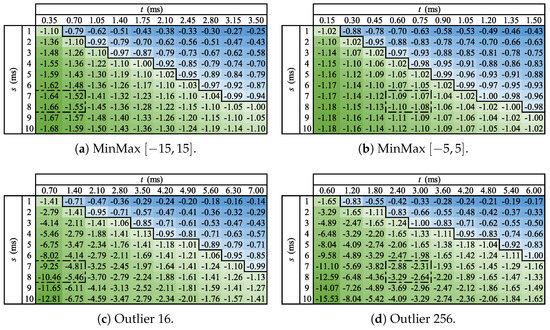
Figure 13.
Slope simulations for each test case using execution time as the cost.
The energy consumption values used in this analysis are the ones obtained for the NodeMCU device. Figure 14a has the MinMax simulation results, for which there is a need to either increase t or decrease s by for cloud computing to become the most profitable choice. Similarly to the results in Figure 13b, the MinMax values displayed in Figure 14b also needs to be adjusted by a much smaller factor than what is required by MinMax in order to change the decision between fog and cloud, that is, we need to increase t or decrease s by only . Again, this can be explained by this case having a higher f than that of MinMax , which brings its initial slope already close to . Figure 14c shows the simulation results for Outlier 16, which require a very large adjustment of to change our decision. Again, this can be explained by the initial slope being far from due to a very low value of f. Figure 14d presents the simulation results for Outlier 256, and here, we need to increase t or decrease s by to change our decision. As in the case of Figure 13d, the low f value of this instance is compensated by a larger t value, which brings its slope to when compared to Outlier 16.
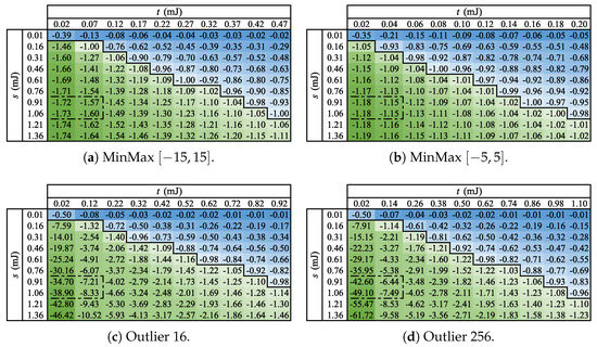
Figure 14.
Slope simulations for each test case using energy consumption as the cost.
Lastly, it is relevant to point out that we also simulated all of these cases employing the real f values. Although that leads us to slightly different slopes, the decision between fog and cloud stays the same in all scenarios. If we had used a smaller value for the maximum increase in cost allowed, we would have seen some marginal discrepancies in borderline cases (i.e., cases where the slope is very close to ), as f would have been less precise due to being estimated using fewer data points. Divergences can also occur due to rounding differences in borderline cases. We do not consider this an issue, as borderline cases have similar fog and cloud costs.
5. Conclusions
This article introduces two cost models for fog and cloud computing. The first is a mathematical model that can be used to estimate the cost of processing a data stream on the device that collected it (fog computing cost) and the cost of sending the data to be processed in the cloud (cloud computing cost). Both of these costs are calculated from the point of view of the device, as this would allow it to choose where to process the data stream while collecting its elements. The second is a visual model that is a cloud computing cost vs. fog computing cost graph. It intends to help the user decide which of the strategies presents the lowest cost according to a certain metric. Using this visual model, the user can better understand the test cases they are working with and improve the implementation of their processing strategy.
Considering that our models are based on linear equations, we observed that the user can make their decision by analyzing the slope of a line drawn in the visual model. As discussed, fog computing is more profitable in the cases where the slope is less than or equal to , with cloud computing having the lower cost otherwise.
One of the parameters of our model is the probability that a number will pass the filter, which we call f. We analyzed different strategies to estimate this value and observed that looking at a contiguous set of elements at the beginning of the stream is a straightforward approach that yields good estimates. The two other approaches that we tested, which involve continuously monitoring the stream and dynamically adjusting the estimate, presented very little performance gains, not justifying their use.
We applied our models to two instances of a filter that allows numbers outside of a certain range to pass and two instances of a filter that finds outliers in a window of values. We used execution time and energy consumption as the cost types for our analysis and executed the tests on five different datasets (four datasets with real-world climatological data and one dataset with artificial data). By comparing the slope of the linear equation obtained with the real and estimated values of f, we noticed that our estimation process worked well, as it presented an error of less than in most of our test cases and allowed us to decide correctly on the more profitable strategy to process the values in all but one case.
We also simulated a different range of values for our test cases and found out how different parameters would affect our decision. We looked at how much it would be necessary to decrease the time it takes to send the data to the cloud (which we call s) or increase the time it takes to execute the application in the fog (which we call t) for cloud computing to become the more profitable approach in cases where the fog was the chosen solution. When using execution time as the cost type, the values of the parameters had to change from to to affect our decision, and in the case of energy consumption as the cost type, they had to change from up to . We noticed that the size of these alterations depends on factors such as the value of f and how close s and t are to each other. We point out that this type of investigation is very useful to visualize possible changes in technology. Again, our estimation process proved to be effective, as the simulations using the real and predicted values presented the same decisions in all cases.
We intend to continue this research by improving our model to account for scenarios not included in this article, such as splitting tasks and sending data to other nearby devices, and overlapping processing and transferring times. We also plan to test our model using test cases with additional custom code operations. Another interesting path is to not only consider the costs from the point of view of the device, but also to calculate the costs looking at the whole system in order to analyze the impact of employing fog computing in the applications that we are studying. Furthermore, we propose to implement a system that uses our model to choose between processing values in the fog or the cloud, and execute it on constrained devices.
Author Contributions
F.P. and E.B. conceived of and designed the models and experiments; F.P. performed the experiments; F.P. and E.B. analyzed the data; V.M.d.R. contributed materials/analysis tools; F.P. and V.M.d.R. wrote the article.
Funding
The authors would like to thank CAPES (PROCAD 2966/2014), CNPq (140653/2017-1 and 313012/2017-2), and FAPESP (2013/08293-7) for their financial support.
Acknowledgments
The authors would like to thank the Multidisciplinary High Performance Computing Lab for its infrastructure and contributions.
Conflicts of Interest
The authors declare no conflict of interest. The founding sponsors had no role in the design of the study; in the collection, analyses, or interpretation of data; in the writing of the manuscript; nor in the decision to publish the results.
Appendix A. Notation

Table A1.
Notation for the cloud and fog computing cost models.
Table A1.
Notation for the cloud and fog computing cost models.
| Notation | Restriction | Definition |
|---|---|---|
| b | Number of blocks into which the stream is divided to compute several f values along the stream. | |
| Cost of sending the data to be processed in the cloud. | ||
| Cost of processing the data in the fog and sending the data that pass the filter to the cloud. | ||
| f | Probability that a value will pass the filter. | |
| i | Cost of being idle between processing a value and reading the next one. | |
| n | Number of values that passed the filter among the tested values. | |
| p | Penalty for processing a value in the fog when it would cost less to do so in the cloud. | |
| r | Cost of reading a value. | |
| s | Cost of sending a value to the cloud. | |
| t | Cost of executing a custom code that decides if the value should be sent to the cloud. | |
| v | Number of values that we are allowed to test to estimate f considering the maximum increase in cost defined by the user. | |
| z | Stream size (i.e., number of processed values). |
Appendix B. Experimental Data
Table A2.
Execution time results in fog-prone cases.
Table A2.
Execution time results in fog-prone cases.
| Benchmark | Dataset | t (ms) | p (%) | v | n | f (Est.) | f (Real) | Slope (Est.) | Slope (Real) | Slope Error (%) |
|---|---|---|---|---|---|---|---|---|---|---|
| MinMax | HRelHumidity | 0.673551 | 0.000141 | 3551 | 3551 | 1.0000 | 1.0000 | −0.9155 | −0.9155 | −0.0000 |
| HVisibility | 0.614381 | 0.000128 | 3893 | 0 | 0.0000 | 0.0000 | −11.8819 | −11.8819 | −0.0000 | |
| HWBTempC | 0.629857 | 0.000132 | 3797 | 760 | 0.2002 | 0.2784 | −3.4911 | −2.7420 | +27.3195 | |
| HWindSpeed | 0.619163 | 0.000129 | 3863 | 515 | 0.1333 | 0.1393 | −4.5844 | −4.4623 | +2.7351 | |
| Synthetic | 0.635126 | 0.000133 | 3766 | 2108 | 0.5597 | 0.5536 | −1.5462 | −1.5611 | −0.9566 | |
| MinMax | HRelHumidity | 0.673655 | 0.000141 | 3550 | 3550 | 1.0000 | 1.0000 | −0.9155 | −0.9155 | −0.0000 |
| HVisibility | 0.660127 | 0.000138 | 3623 | 2984 | 0.8236 | 0.8336 | −1.0940 | −1.0823 | +1.0881 | |
| HWBTempC | 0.646680 | 0.000135 | 3698 | 2613 | 0.7066 | 0.6911 | −1.2576 | −1.2826 | −1.9489 | |
| HWindSpeed | 0.656031 | 0.000137 | 3646 | 2920 | 0.8009 | 0.8013 | −1.1227 | −1.1222 | +0.0440 | |
| Synthetic | 0.643882 | 0.000135 | 3715 | 3087 | 0.8310 | 0.8299 | −1.0880 | −1.0892 | −0.1187 | |
| Outlier 16 | HRelHumidity | 0.715757 | 0.000150 | 3342 | 73 | 0.0218 | 0.0236 | −8.3408 | −8.2180 | +1.4952 |
| HVisibility | 0.667375 | 0.000139 | 3584 | 355 | 0.0991 | 0.0911 | −5.2501 | −5.4794 | −4.1852 | |
| HWBTempC | 0.723876 | 0.000151 | 3304 | 65 | 0.0197 | 0.0222 | −8.4151 | −8.2367 | +2.1662 | |
| HWindSpeed | 0.719371 | 0.000150 | 3325 | 121 | 0.0364 | 0.0267 | −7.4110 | −7.9862 | −7.2024 | |
| Synthetic | 0.741199 | 0.000155 | 3227 | 26 | 0.0081 | 0.0076 | −9.1248 | −9.1606 | −0.3902 | |
| Outlier 256 | HRelHumidity | 2.590709 | 0.000542 | 923 | 41 | 0.0444 | 0.0051 | −2.5043 | −2.7776 | −9.8403 |
| HVisibility | 1.729101 | 0.000361 | 1383 | 215 | 0.1555 | 0.1112 | −2.5489 | −2.8731 | −11.2837 | |
| HWBTempC | 2.561749 | 0.000535 | 933 | 15 | 0.0161 | 0.0124 | −2.7248 | −2.7522 | −0.9963 | |
| HWindSpeed | 2.454752 | 0.000513 | 974 | 5 | 0.0051 | 0.0160 | −2.9291 | −2.8386 | +3.1893 | |
| Synthetic | 2.633129 | 0.000550 | 908 | 4 | 0.0044 | 0.0012 | −2.7389 | −2.7629 | −0.8681 |
Table A3.
Execution time results in cloud-prone cases.
Table A3.
Execution time results in cloud-prone cases.
| Benchmark | Dataset | t (ms) | p (%) | v | n | f (Est.) | f (Real) | Slope (Est.) | Slope (Real) | Slope Error (%) |
|---|---|---|---|---|---|---|---|---|---|---|
| MinMax | HRelHumidity | 0.673551 | 0.001408 | 355 | 355 | 1.0000 | 1.0000 | −0.5201 | −0.5201 | −0.0000 |
| HVisibility | 0.614381 | 0.001284 | 389 | 0 | 0.0000 | 0.0000 | −1.1882 | −1.1882 | −0.0000 | |
| HWBTempC | 0.629857 | 0.001317 | 379 | 210 | 0.5541 | 0.2784 | −0.7058 | −0.8762 | −19.4563 | |
| HWindSpeed | 0.619163 | 0.001294 | 386 | 7 | 0.0181 | 0.1393 | −1.1543 | −1.0127 | +13.9844 | |
| Synthetic | 0.635126 | 0.001328 | 376 | 206 | 0.5479 | 0.5536 | −0.7053 | −0.7024 | +0.4010 | |
| MinMax | HRelHumidity | 0.673655 | 0.001408 | 355 | 355 | 1.0000 | 1.0000 | −0.5201 | −0.5201 | −0.0000 |
| HVisibility | 0.660127 | 0.001380 | 362 | 302 | 0.8343 | 0.8336 | −0.5752 | −0.5754 | −0.0392 | |
| HWBTempC | 0.646680 | 0.001352 | 369 | 369 | 1.0000 | 0.6911 | −0.5303 | −0.6341 | −16.3797 | |
| HWindSpeed | 0.656031 | 0.001371 | 364 | 275 | 0.7555 | 0.8013 | −0.6045 | −0.5883 | +2.7673 | |
| Synthetic | 0.643882 | 0.001346 | 371 | 308 | 0.8302 | 0.8299 | −0.5840 | −0.5841 | −0.0189 | |
| Outlier 16 | HRelHumidity | 0.715757 | 0.001496 | 334 | 10 | 0.0299 | 0.0236 | −0.9897 | −0.9959 | −0.6239 |
| HVisibility | 0.667375 | 0.001395 | 358 | 43 | 0.1201 | 0.0911 | −0.9668 | −0.9947 | −2.8069 | |
| HWBTempC | 0.723876 | 0.001513 | 330 | 5 | 0.0152 | 0.0222 | −0.9933 | −0.9863 | +0.7048 | |
| HWindSpeed | 0.719371 | 0.001504 | 332 | 10 | 0.0301 | 0.0267 | −0.9847 | −0.9880 | −0.3395 | |
| Synthetic | 0.741199 | 0.001549 | 322 | 1 | 0.0031 | 0.0076 | −0.9819 | −0.9775 | +0.4442 | |
| Outlier 256 | HRelHumidity | 2.590709 | 0.005415 | 92 | 0 | 0.0000 | 0.0051 | −0.2818 | −0.2814 | +0.1445 |
| HVisibility | 1.729101 | 0.003614 | 138 | 55 | 0.3986 | 0.1112 | −0.3614 | −0.4033 | −10.3846 | |
| HWBTempC | 2.561749 | 0.005355 | 93 | 0 | 0.0000 | 0.0124 | −0.2850 | −0.2840 | +0.3539 | |
| HWindSpeed | 2.454752 | 0.005131 | 97 | 0 | 0.0000 | 0.0160 | −0.2974 | −0.2960 | +0.4765 | |
| Synthetic | 2.633129 | 0.005504 | 90 | 1 | 0.0111 | 0.0012 | −0.2764 | −0.2771 | −0.2729 |
Table A4.
NodeMCU energy consumption results in fog-prone cases.
Table A4.
NodeMCU energy consumption results in fog-prone cases.
| Benchmark | Dataset | t (mJ) | p (%) | v | n | f (Est.) | f (Real) | Slope (Est.) | Slope (Real) | Slope Error (%) |
|---|---|---|---|---|---|---|---|---|---|---|
| MinMax | HRelHumidity | 0.023170 | 0.000035 | 14,453 | 14,453 | 1.0000 | 1.0000 | −0.9778 | −0.9778 | −0.0000 |
| HVisibility | 0.021135 | 0.000032 | 15,845 | 0 | 0.0000 | 0.0000 | −48.3565 | −48.3565 | −0.0000 | |
| HWBTempC | 0.021667 | 0.000032 | 15,456 | 3920 | 0.2536 | 0.2784 | −3.6387 | −3.3376 | +9.0198 | |
| HWindSpeed | 0.021299 | 0.000032 | 15,723 | 2131 | 0.1355 | 0.1393 | −6.3949 | −6.2452 | +2.3970 | |
| Synthetic | 0.021848 | 0.000033 | 15,327 | 8567 | 0.5589 | 0.5536 | −1.7232 | −1.7393 | −0.9288 | |
| MinMax | HRelHumidity | 0.023174 | 0.000035 | 14,451 | 14,451 | 1.0000 | 1.0000 | −0.9778 | −0.9778 | −0.0000 |
| HVisibility | 0.022708 | 0.000034 | 14,747 | 12,184 | 0.8262 | 0.8336 | −1.1787 | −1.1685 | +0.8687 | |
| HWBTempC | 0.022246 | 0.000033 | 15,054 | 11,189 | 0.7433 | 0.6911 | −1.3071 | −1.4028 | −6.8176 | |
| HWindSpeed | 0.022567 | 0.000034 | 14,839 | 11,701 | 0.7885 | 0.8013 | −1.2336 | −1.2145 | +1.5716 | |
| Synthetic | 0.022150 | 0.000033 | 15,119 | 12,530 | 0.8288 | 0.8299 | −1.1759 | −1.1743 | +0.1301 | |
| Outlier 16 | HRelHumidity | 0.024622 | 0.000037 | 13,601 | 324 | 0.0238 | 0.0236 | −20.8708 | −20.9521 | −0.3880 |
| HVisibility | 0.022958 | 0.000034 | 14,587 | 1470 | 0.1008 | 0.0911 | −8.1144 | −8.8072 | −7.8668 | |
| HWBTempC | 0.024901 | 0.000037 | 13,448 | 297 | 0.0221 | 0.0222 | −21.5284 | −21.4534 | +0.3493 | |
| HWindSpeed | 0.024746 | 0.000037 | 13,532 | 409 | 0.0302 | 0.0267 | −18.3694 | −19.6518 | −6.5253 | |
| Synthetic | 0.025497 | 0.000038 | 13,134 | 90 | 0.0069 | 0.0076 | −31.4457 | −30.6958 | +2.4432 | |
| Outlier 256 | HRelHumidity | 0.089120 | 0.000133 | 3757 | 47 | 0.0125 | 0.0051 | −10.0289 | −10.8308 | −7.4044 |
| HVisibility | 0.059481 | 0.000089 | 5630 | 531 | 0.0943 | 0.1112 | −6.5567 | −5.9035 | +11.0641 | |
| HWBTempC | 0.088124 | 0.000132 | 3800 | 15 | 0.0039 | 0.0124 | −11.0896 | −10.1371 | +9.3965 | |
| HWindSpeed | 0.084443 | 0.000126 | 3965 | 52 | 0.0131 | 0.0160 | −10.4449 | −10.1371 | +3.0363 | |
| Synthetic | 0.090580 | 0.000135 | 3697 | 5 | 0.0014 | 0.0012 | −11.1133 | −11.1277 | −0.1295 |
Table A5.
NodeMCU energy consumption results in cloud-prone cases.
Table A5.
NodeMCU energy consumption results in cloud-prone cases.
| Benchmark | Dataset | t (mJ) | p (%) | v | n | f (Est.) | f (Real) | Slope (Est.) | Slope (Real) | Slope Error (%) |
|---|---|---|---|---|---|---|---|---|---|---|
| MinMax | HRelHumidity | 0.023170 | 0.001384 | 361 | 361 | 1.0000 | 1.0000 | −0.5244 | −0.5244 | −0.0000 |
| HVisibility | 0.021135 | 0.001262 | 396 | 0 | 0.0000 | 0.0000 | −1.2089 | −1.2089 | −0.0000 | |
| HWBTempC | 0.021667 | 0.001294 | 386 | 217 | 0.5622 | 0.2784 | −0.7091 | −0.8878 | −20.1222 | |
| HWindSpeed | 0.021299 | 0.001272 | 393 | 7 | 0.0178 | 0.1393 | −1.1745 | −1.0278 | +14.2665 | |
| Synthetic | 0.021848 | 0.001305 | 383 | 209 | 0.5457 | 0.5536 | −0.7139 | −0.7099 | +0.5616 | |
| MinMax | HRelHumidity | 0.023174 | 0.001384 | 361 | 361 | 1.0000 | 1.0000 | −0.5244 | −0.5244 | −0.0000 |
| HVisibility | 0.022708 | 0.001356 | 368 | 304 | 0.8261 | 0.8336 | −0.5831 | −0.5806 | +0.4365 | |
| HWBTempC | 0.022246 | 0.001329 | 376 | 376 | 1.0000 | 0.6911 | −0.5346 | −0.6403 | −16.5127 | |
| HWindSpeed | 0.022567 | 0.001348 | 370 | 280 | 0.7568 | 0.8013 | −0.6097 | −0.5936 | +2.7142 | |
| Synthetic | 0.022150 | 0.001323 | 377 | 312 | 0.8276 | 0.8299 | −0.5901 | −0.5894 | +0.1345 | |
| Outlier 16 | HRelHumidity | 0.024622 | 0.001470 | 340 | 10 | 0.0294 | 0.0236 | −1.0070 | −1.0128 | −0.5816 |
| HVisibility | 0.022958 | 0.001371 | 364 | 43 | 0.1181 | 0.0911 | −0.9836 | −1.0105 | −2.6609 | |
| HWBTempC | 0.024901 | 0.001487 | 336 | 5 | 0.0149 | 0.0222 | −1.0106 | −1.0032 | +0.7445 | |
| HWindSpeed | 0.024746 | 0.001478 | 338 | 10 | 0.0296 | 0.0267 | −1.0019 | −1.0048 | −0.2919 | |
| Synthetic | 0.025497 | 0.001523 | 328 | 1 | 0.0030 | 0.0076 | −0.9990 | −0.9945 | +0.4576 | |
| Outlier 256 | HRelHumidity | 0.089120 | 0.005322 | 93 | 0 | 0.0000 | 0.0051 | −0.2867 | −0.2863 | +0.1470 |
| HVisibility | 0.059481 | 0.003552 | 140 | 55 | 0.3929 | 0.1112 | −0.3675 | −0.4100 | −10.3520 | |
| HWBTempC | 0.088124 | 0.005263 | 95 | 0 | 0.0000 | 0.0124 | −0.2899 | −0.2889 | +0.3601 | |
| HWindSpeed | 0.084443 | 0.005043 | 99 | 0 | 0.0000 | 0.0160 | −0.3026 | −0.3011 | +0.4848 | |
| Synthetic | 0.090580 | 0.005410 | 92 | 1 | 0.0109 | 0.0012 | −0.2812 | −0.2820 | −0.2709 |
Table A6.
Raspberry Pi 3 energy consumption results in fog-prone cases.
Table A6.
Raspberry Pi 3 energy consumption results in fog-prone cases.
| Benchmark | Dataset | Instruction Count | t (mJ) | p (%) | v | n | f (Est.) | f (Real) | Slope (Est.) | Slope (Real) | Slope Error (%) |
|---|---|---|---|---|---|---|---|---|---|---|---|
| MinMax | HRelHumidity | 3,997,730 | 0.003321 | 0.000000 | 23,765 | 23,765 | 1.0000 | 1.0000 | −0.9997 | −0.9997 | −0.0000 |
| HVisibility | 2,687,010 | 0.002232 | 0.000000 | 35,358 | 0 | 0.0000 | 0.0000 | −5395.3493 | −5395.3493 | −0.0000 | |
| HWBTempC | 3,047,723 | 0.002532 | 0.000000 | 31,174 | 7744 | 0.2484 | 0.2784 | −4.0222 | −3.5891 | +12.0664 | |
| HWindSpeed | 2,869,570 | 0.002384 | 0.000000 | 33,109 | 4541 | 0.1372 | 0.1393 | −7.2806 | −7.1695 | +1.5502 | |
| Synthetic | 3,285,947 | 0.002730 | 0.000000 | 28,914 | 16,086 | 0.5563 | 0.5536 | −1.7967 | −1.8058 | −0.4997 | |
| MinMax | HRelHumidity | 3,997,730 | 0.003321 | 0.000000 | 23,765 | 23,765 | 1.0000 | 1.0000 | −0.9997 | −0.9997 | −0.0000 |
| HVisibility | 3,779,590 | 0.003140 | 0.000000 | 25,137 | 20,454 | 0.8137 | 0.8336 | −1.2286 | −1.1993 | +2.4413 | |
| HWBTempC | 3,537,571 | 0.002939 | 0.000000 | 26,857 | 19,474 | 0.7251 | 0.6911 | −1.3787 | −1.4465 | −4.6872 | |
| HWindSpeed | 3,737,250 | 0.003105 | 0.000000 | 25,422 | 20,039 | 0.7883 | 0.8013 | −1.2682 | −1.2476 | +1.6506 | |
| Synthetic | 3,584,428 | 0.002978 | 0.000000 | 26,506 | 22,025 | 0.8309 | 0.8299 | −1.2031 | −1.2047 | −0.1299 | |
| Outlier 16 | HRelHumidity | 6,972,197 | 0.006372 | 0.000001 | 12,388 | 273 | 0.0220 | 0.0236 | −44.3135 | −41.3824 | +7.0831 |
| HVisibility | 6,035,976 | 0.005516 | 0.000001 | 14,309 | 1441 | 0.1007 | 0.0911 | −9.8850 | −10.9245 | −9.5154 | |
| HWBTempC | 7,285,119 | 0.006658 | 0.000001 | 11,856 | 258 | 0.0218 | 0.0222 | −44.8151 | −43.8595 | +2.1788 | |
| HWindSpeed | 7,045,547 | 0.006439 | 0.000001 | 12,259 | 369 | 0.0301 | 0.0267 | −32.6425 | −36.7553 | −11.1898 | |
| Synthetic | 7,384,825 | 0.006749 | 0.000001 | 11,695 | 80 | 0.0068 | 0.0076 | −135.1194 | −122.1042 | +10.6591 | |
| Outlier 256 | HRelHumidity | 49,584,961 | 0.045317 | 0.000006 | 1741 | 41 | 0.0235 | 0.0051 | −36.6140 | −112.4953 | −67.4529 |
| HVisibility | 30,115,961 | 0.027524 | 0.000003 | 2868 | 459 | 0.1600 | 0.1112 | −6.1604 | −8.8124 | −30.0942 | |
| HWBTempC | 49,178,545 | 0.044946 | 0.000006 | 1756 | 15 | 0.0085 | 0.0124 | −81.4756 | −61.9114 | +31.6004 | |
| HWindSpeed | 46,647,122 | 0.042632 | 0.000005 | 1851 | 52 | 0.0281 | 0.0160 | −31.6132 | −51.1218 | −38.1610 | |
| Synthetic | 50,492,036 | 0.046146 | 0.000006 | 1710 | 4 | 0.0023 | 0.0012 | −162.0664 | −197.3519 | −17.8795 |
Table A7.
Raspberry Pi 3 energy consumption results in cloud-prone cases.
Table A7.
Raspberry Pi 3 energy consumption results in cloud-prone cases.
| Benchmark | Dataset | Instruction Count | t (mJ) | p (%) | v | n | f (Est.) | f (Real) | Slope (Est.) | Slope (Real) | Slope Error (%) |
|---|---|---|---|---|---|---|---|---|---|---|---|
| MinMax | HRelHumidity | 3,997,730 | 0.003321 | 0.001683 | 594 | 594 | 1.0000 | 1.0000 | −0.4755 | −0.4755 | −0.0000 |
| HVisibility | 2,687,010 | 0.002232 | 0.001131 | 883 | 0 | 0.0000 | 0.0000 | −1.3488 | −1.3488 | −0.0000 | |
| HWBTempC | 3,047,723 | 0.002532 | 0.001283 | 779 | 482 | 0.6187 | 0.2784 | −0.6851 | −0.8934 | −23.3159 | |
| HWindSpeed | 2,869,570 | 0.002384 | 0.001208 | 827 | 12 | 0.0145 | 0.1393 | −1.2403 | −1.0741 | +15.4754 | |
| Synthetic | 3,285,947 | 0.002730 | 0.001383 | 722 | 403 | 0.5582 | 0.5536 | −0.6827 | −0.6848 | −0.3149 | |
| MinMax | HRelHumidity | 3,997,730 | 0.003321 | 0.001683 | 594 | 594 | 1.0000 | 1.0000 | −0.4755 | −0.4755 | −0.0000 |
| HVisibility | 3,779,590 | 0.003140 | 0.001591 | 628 | 491 | 0.7818 | 0.8336 | −0.5480 | −0.5329 | +2.8348 | |
| HWBTempC | 3,537,571 | 0.002939 | 0.001489 | 671 | 671 | 1.0000 | 0.6911 | −0.5061 | −0.5998 | −15.6321 | |
| HWindSpeed | 3,737,250 | 0.003105 | 0.001573 | 635 | 484 | 0.7622 | 0.8013 | −0.5576 | −0.5457 | +2.1783 | |
| Synthetic | 3,584,428 | 0.002978 | 0.001509 | 662 | 550 | 0.8308 | 0.8299 | −0.5495 | −0.5498 | −0.0523 | |
| Outlier 16 | HRelHumidity | 6,972,197 | 0.006372 | 0.003229 | 309 | 10 | 0.0324 | 0.0236 | −0.4655 | −0.4674 | −0.4062 |
| HVisibility | 6,035,976 | 0.005516 | 0.002795 | 357 | 43 | 0.1204 | 0.0911 | −0.5122 | −0.5200 | −1.5042 | |
| HWBTempC | 7,285,119 | 0.006658 | 0.003374 | 296 | 5 | 0.0169 | 0.0222 | −0.4488 | −0.4478 | +0.2404 | |
| HWindSpeed | 7,045,547 | 0.006439 | 0.003263 | 306 | 10 | 0.0327 | 0.0267 | −0.4606 | −0.4619 | −0.2767 | |
| Synthetic | 7,384,825 | 0.006749 | 0.003420 | 292 | 1 | 0.0034 | 0.0076 | −0.4455 | −0.4447 | +0.1873 | |
| Outlier 256 | HRelHumidity | 49,584,961 | 0.045317 | 0.022963 | 43 | 0 | 0.0000 | 0.0051 | −0.0664 | −0.0664 | +0.0341 |
| HVisibility | 30,115,961 | 0.027524 | 0.013947 | 71 | 55 | 0.7746 | 0.1112 | −0.1009 | −0.1081 | −6.6915 | |
| HWBTempC | 49,178,545 | 0.044946 | 0.022775 | 43 | 0 | 0.0000 | 0.0124 | −0.0670 | −0.0669 | +0.0832 | |
| HWindSpeed | 46,647,122 | 0.042632 | 0.021603 | 46 | 0 | 0.0000 | 0.0160 | −0.0706 | −0.0706 | +0.1132 | |
| Synthetic | 50,492,036 | 0.046146 | 0.023383 | 42 | 1 | 0.0238 | 0.0012 | −0.0652 | −0.0652 | −0.1471 |
References
- Lucero, S. IoT Platforms: Enabling the Internet of Things; Technical Report; IHS Technology: London, UK, 2016. [Google Scholar]
- Bonomi, F.; Milito, R.; Zhu, J.; Addepalli, S. Fog Computing and Its Role in the Internet of Things. In Proceedings of the 1st MCC Workshop on Mobile Cloud Computing, Helsinki, Finland, 17 August 2012; pp. 13–16. [Google Scholar] [CrossRef]
- Vaquero, L.M.; Rodero-Merino, L. Finding your Way in the Fog: Towards a Comprehensive Definition of Fog Computing. ACM SIGCOMM Comput. Commun. Rev. 2014, 44, 27–32. [Google Scholar] [CrossRef]
- Li, Z.; Wang, C.; Xu, R. Computation Offloading to Save Energy on Handheld Devices: A Partition Scheme. In Proceedings of the 2001 International Conference on Compilers, Architecture, and Synthesis for Embedded Systems, Atlanta, GA, USA, 16–17 November 2001; pp. 238–246. [Google Scholar] [CrossRef]
- Li, Z.; Wang, C.; Xu, R. Task Allocation for Distributed Multimedia Processing on Wirelessly Networked Handheld Devices. In Proceedings of the 16th International Parallel and Distributed Processing Symposium, Ft. Lauderdale, FL, USA, 15–19 April 2001. [Google Scholar] [CrossRef]
- Li, Z.; Xu, R. Energy Impact of Secure Computation on a Handheld Device. In Proceedings of the 2002 IEEE International Workshop on Workload Characterization, Austin, TX, USA, 25 November 2002; pp. 109–117. [Google Scholar] [CrossRef]
- Kremer, U.; Hicks, J.; Rehg, J. A Compilation Framework for Power and Energy Management on Mobile Computers. In International Workshop on Languages and Compilers for Parallel Computing; Springer: Berlin/Heidelberg, Germany, 2003; pp. 115–131. [Google Scholar] [CrossRef]
- Rong, P.; Pedram, M. Extending the Lifetime of a Network of Battery-Powered Mobile Devices by Remote Processing: A Markovian Decision-based Approach. In Proceedings of the 2003 Design Automation Conference, Anaheim, CA, USA, 2–6 June 2003; pp. 906–911. [Google Scholar] [CrossRef]
- Chen, G.; Kang, B.-T.; Kandemir, M.; Vijaykrishnan, N.; Irwin, M.J.; Chandramouli, R. Studying Energy Trade Offs in Offloading Computation/Compilation in Java-Enabled Mobile Devices. IEEE Trans. Parallel Distrib. Syst. 2004, 15, 795–809. [Google Scholar] [CrossRef]
- O’Hara, K.J.; Nathuji, R.; Raj, H.; Schwan, K.; Balch, T. AutoPower: Toward Energy-Aware Software Systems for Distributed Mobile Robots. In Proceedings of the 2006 IEEE International Conference on Robotics and Automation, Orlando, FL, USA, 15–19 May 2006; pp. 2757–2762. [Google Scholar] [CrossRef]
- Xian, C.; Lu, Y.-H.; Li, Z. Adaptive Computation Offloading for Energy Conservation on Battery-Powered Systems. In Proceedings of the 2007 International Conference on Parallel and Distributed Systems, Hsinchu, Taiwan, 5–7 December 2007; pp. 1–8. [Google Scholar] [CrossRef]
- Hong, Y.-J.; Kumar, K.; Lu, Y.-H. Energy Efficient Content-Based Image Retrieval for Mobile Systems. In Proceedings of the IEEE International Symposium on Circuits and Systems, Taipei, Taiwan, 24–27 May 2009; pp. 1673–1676. [Google Scholar] [CrossRef]
- Gu, X.; Nahrstedt, K.; Messer, A.; Greenberg, I.; Milojicic, D. Adaptive Offloading Inference for Delivering Applications in Pervasive Computing Environments. In Proceedings of the First IEEE International Conference on Pervasive Computing and Communications, Fort Worth, TX, USA, 26 March 2003; pp. 107–114. [Google Scholar] [CrossRef]
- Gurun, S.; Krintz, C.; Wolski, R. NWSLite: A Light-Weight Prediction Utility for Mobile Devices. In Proceedings of the 2nd International Conference on Mobile Systems, Applications, and Services, Boston, MA, USA, 6–9 June 2004; pp. 2–11. [Google Scholar] [CrossRef]
- Wang, C.; Li, Z. Parametric Analysis for Adaptive Computation Offloading. In Proceedings of the 2004 Conference on Programming Language Design and Implementation, Washington, DC, USA, 9–11 June 2004; pp. 119–130. [Google Scholar] [CrossRef]
- Wolski, R.; Gurun, S.; Krintz, C.; Nurmi, D. Using Bandwidth Data To Make Computation Offloading Decisions. In Proceedings of the 2008 IEEE International Symposium on Parallel and Distributed Processing, Miami, FL, USA, 14–18 April 2008; pp. 1–8. [Google Scholar] [CrossRef]
- Nimmagadda, Y.; Kumar, K.; Lu, Y.-H.; Lee, C.S.G. Real-time Moving Object Recognition and Tracking Using Computation Offloading. In Proceedings of the 2010 IEEE/RSJ International Conference on Intelligent Robots and Systems, Taipei, Taiwan, 18–22 October 2010; pp. 2449–2455. [Google Scholar] [CrossRef]
- Jayaraman, P.P.; Gomes, J.B.; Nguyen, H.L.; Abdallah, Z.S.; Krishnaswamy, S.; Zaslavsky, A. CARDAP: A Scalable Energy-Efficient Context Aware Distributed Mobile Data Analytics Platform for the Fog. In East European Conference on Advances in Databases and Information Systems; Springer: Cham, Switzerland, 2014; pp. 192–206. [Google Scholar] [CrossRef]
- Deng, R.; Lu, R.; Lai, C.; Luan, T.H.; Liang, H. Optimal Workload Allocation in Fog-Cloud Computing Toward Balanced Delay and Power Consumption. IEEE Internet Things J. 2016, 3, 1171–1181. [Google Scholar] [CrossRef]
- Xu, J.; Ren, S. Online Learning for Offloading and Autoscaling in Renewable-Powered Mobile Edge Computing. In Proceedings of the 2016 IEEE Global Communications Conference, Washington, DC, USA, 4–8 December 2016; pp. 1–6. [Google Scholar] [CrossRef]
- Liu, L.; Chang, Z.; Guo, X.; Mao, S.; Ristaniemi, T. Multiobjective Optimization for Computation Offloading in Fog Computing. IEEE Internet Things J. 2018, 5, 283–294. [Google Scholar] [CrossRef]
- Williams, S.; Waterman, A.; Patterson, D. Roofline: An Insightful Visual Performance Model for Multicore Architectures. Commun. ACM 2009, 52, 65–76. [Google Scholar] [CrossRef]
- Pisani, F.; Brunetta, J.R.; do Rosario, V.M.; Borin, E. Beyond the Fog: Bringing Cross-Platform Code Execution to Constrained IoT Devices. In Proceedings of the 29th International Symposium on Computer Architecture and High Performance Computing, Campinas, Brazil, 17–20 October 2017; pp. 17–24. [Google Scholar] [CrossRef]
- Do Rosario, V.M.; Pisani, F.; Gomes, A.R.; Borin, E. Fog-Assisted Translation: Towards Efficient Software Emulation on Heterogeneous IoT Devices. In Proceedings of the 2018 IEEE International Parallel and Distributed Processing Symposium Workshops, Vancouver, BC, Canada, 21–25 May 2018; pp. 1268–1277. [Google Scholar] [CrossRef]
- Hoaglin, D.C.; Iglewicz, B.; Tukey, J.W. Performance of Some Resistant Rules for Outlier Labeling. J. Am. Stat. Assoc. 1986, 81, 991–999. [Google Scholar] [CrossRef]
- National Centers for Environmental Information. Climate Data Online: Dataset Discovery. Available online: https://www.ncdc.noaa.gov/cdo-web/datasets#LCD (accessed on 23 August 2018).
- Mocnej, J.; Miškuf, M.; Papcun, P.; Zolotová, I. Impact of Edge Computing Paradigm on Energy Consumption in IoT. IFAC-PapersOnLine 2018, 51, 162–167. [Google Scholar] [CrossRef]
- Dezfouli, B.; Amirtharaj, I.; Li, C.-C. EMPIOT: An Energy Measurement Platform for Wireless IoT Devices. J. Netw. Comput. Appl. 2018, 121, 135–148. [Google Scholar] [CrossRef]
© 2019 by the authors. Licensee MDPI, Basel, Switzerland. This article is an open access article distributed under the terms and conditions of the Creative Commons Attribution (CC BY) license (http://creativecommons.org/licenses/by/4.0/).