Learning Dynamic Factors to Improve the Accuracy of Bus Arrival Time Prediction via a Recurrent Neural Network

Abstract

Accurate prediction of bus arrival times is a challenging problem in the public transportation field. Previous studies have shown that to improve prediction accuracy, more heterogeneous measurements provide better results. So what other factors should be added into the prediction model? Traditional prediction methods mainly use the arrival time and the distance between stations, but do not make full use of dynamic factors such as passenger number, dwell time, bus driving efficiency, etc. We propose a novel approach that takes full advantage of dynamic factors. Our approach is based on a Recurrent Neural Network (RNN). The experimental results indicate that a variety of prediction algorithms (such as Support Vector Machine, Kalman filter, Multilayer Perceptron, and RNN) have significantly improved performance after using dynamic factors. Further, we introduce RNN with an attention mechanism to adaptively select the most relevant input factors. Experiments demonstrate that the prediction accuracy of RNN with an attention mechanism is better than RNN with no attention mechanism when there are heterogeneous input factors. The experimental results show the superior performances of our approach on the data set provided by Jinan Public Transportation Corporation.

1. Introduction

Accurate prediction of bus arrival times is of great significance for urban public transportation planning, real-time bus scheduling, and facilitating public travel. Some mobile map apps have the ability to predict the arrival time of a bus. However, the current accuracy of prediction cannot fully meet the needs of travelers.

Currently, there are many ways to predict bus arrival times. Kalman filtering is a common method for bus arrival time prediction [1,2]. In reference [3], the Godunov scheme is used in the prediction scheme based on the Kalman filter. Support Vector Machine (SVM) [4] is widely used in this task. In the proposed methods, SVM is combined with a Genetic Algorithm [5], Kalman filter [6], and artificial neural network (ANN) [7], respectively. In addition to Kalman filtering and SVM, there are other time series prediction methods, such as road segment average travel time [8], the Relevance Vector Machine Regression [9], clustering [10], Queueing Theory combined with Machine Learning [11], and Random Forests [12]. Artificial neural networks have been widely used in various research fields in recent years [13,14,15]. Among artificial neural networks, Multilayer Perceptron (MLP) [16] and Recurrent Neural Network (RNN) [17] have been used to predict bus arrival time. The above methods are of great value to the overall planning of the bus route, but have not yet met the more sensitive time requirements of some tasks such as estimation of passenger waiting time and real-time scheduling of buses. So, the question becomes how can we further improve the accuracy of bus arrival time prediction?

Previous studies have shown that to improve prediction accuracy, more heterogeneous measurements are better [17]. What other factors should be input into the prediction model? Traditional bus arrival time prediction methods only use information that does not change in a short period of time, such as the distance between stations, the number of intersections, and the number of traffic lights. In the bus operation process, the arrival time is also affected by some dynamic factors, such as the number of passengers, traffic conditions, weather, etc. The dynamic information is constantly changing as the bus travels and cannot be obtained directly from the map. Existing prediction methods choose to ignore these dynamic factors when modeling.

In order to further improve the accuracy of prediction, we propose a novel approach that takes full advantage of dynamic factors. We built a data set containing dynamic factors based on the raw data provided by Jinan Public Transportation Corporation and experimented with this dataset using a variety of algorithms. The experimental results show that the prediction accuracy of these methods has been improved significantly after making full use of the dynamic factors. Among the methods discussed, the RNN methods have the higher prediction accuracy. The main reason for this is that RNN has the ability to capture long-term dependencies. On this basis, we further explored the impact of the structure of RNN on the prediction results, and found that DA-RNN (Dual-stage Attention-based Recurrent Neural Network) [18] performed better than the classic Long Short-Term Memory RNN (LSTM RNN) in the task. Compared with LSTM RNN, DA-RNN has a better attention mechanism. An attention mechanism can select the critical factors for the prediction from the input data and capture the long-range temporal information.

Our main contributions are summarized as follows:

• We find that dynamic factors in the model input can improve the accuracy of bus arrival time prediction. To this end, we have established a data set that contains dynamic factors. The experimental results show that a variety of prediction algorithms (such as SVM, Kalman filter, MLP and RNN) have significantly improved performance after using dynamic factors.
• We introduce the attention mechanism to adaptively select the most relevant factors from heterogeneous information. Experiments show that the prediction accuracy of RNN with an attention mechanism is better than RNN with no attention mechanism when there are heterogeneous input factors.

2. Problem Formulation

For the bus arrival time prediction problem, the departure time, when the bus departs from the originating station, can be regarded as a known variable. As long as the travel time between any two adjacent stations of the entire line is accurately predicted, we can accumulate them and add the sum to the departure time to get the arrival time of any station. Therefore, the arrival time prediction can be converted into a travel time prediction.

Suppose there are N sites on the route of a certain bus. Then the route can be divided into N − 1 road segments. The arrival time of the i-th station is t_i (i = 1, 2... N). The travel time of the i-th road segment is y_i. The relationship between travel time y and arrival time t is:

$$y_i=t_{i+1}-t_i,i=1,2,\dots N-1.$$

(1)

We divide the factors affecting bus arrival time into static and dynamic factors. Static factors can be expressed as:

$$x_{Si}=(d_i,c_i,l_i,b_i)$$

(2)

where d_i is the length of the i-th road segment, c_i is the number of intersections, l_i is the number of lanes, and b_i indicates whether a bus lane exists (b_i can be “1” or “0”; “1” means “yes”, “0” means “no”).

Dynamic factors can be expressed as:

$$x_{Di}=(t{d}_i,n_i,E_i)$$

(3)

where td_i is the dwell time of the i-th station, n_i is the passenger number of the i-th road segment, E_i is bus driving efficiency of the i-th road segment. In previous research [19], we proposed a method to measure the efficiency of bus driving. The calculation method of E_i is:

$$E_i=\frac{n_i}{y_i(1+\lambda {(\frac{n_i}{n_{\max }})}^{\omega })}.$$

(4)

The travel time $y_i$ is predicted by the data of the last T road segments. The prediction formula for the travel time is:

$${\widehat{y}}_i=F_1(x_{S(i-T+1)},\dots ,x_{Si},x_D{}_{(i-T+1)},\dots ,x_{Di},y_{(i-T+1)},\dots ,y_{(i-1)}),$$

(5)

$${\widehat{y}}_{(i+1)}=F_2(x_{S(i-T+2)},\dots ,x_{Si},x_{S(i+1)},y_{(i-T+2)},\dots ,y_{(i-1)},{\widehat{y}}_i),$$

(6)

⋯

$${\widehat{y}}_{(i+k)}=F_2(x_{S(i-T+1+k)},\dots ,x_{S(i+k)},y_{(i-T+1+k)},\dots ,{\widehat{y}}_{(i+k-2)},{\widehat{y}}_{(i+k-1)}),$$

(7)

⋯

$${\widehat{y}}_{(N-1)}=F_2(x_{S(N-T)},\dots ,x_{S(N-1)},y_{(N-T)},\dots ,{\widehat{y}}_{(N-3)},{\widehat{y}}_{(N-2)}).$$

(8)

${\widehat{y}}_i$ is the prediction of the current road segment based on both static and dynamic factors. The values from ${\widehat{y}}_{(i+1)}$ to ${\widehat{y}}_{(N-1)}$ are the prediction of the remaining road segments, and dynamic factors are not available in these cases. F₁ and F₂ represent two prediction models which have different inputs and structures. When i < T, historical data will be entered into the prediction model to ensure that the length of the input data sequence is T.

After setting the bus on the i-th road segment, the arrival time of the k-th station is $t_k$:

$$t_k=t_{i-1}+{\displaystyle \sum _{n=i}^k{\widehat{y}}_n},i\le k\le N.$$

(9)

3. Prediction Framework

3.1. Model

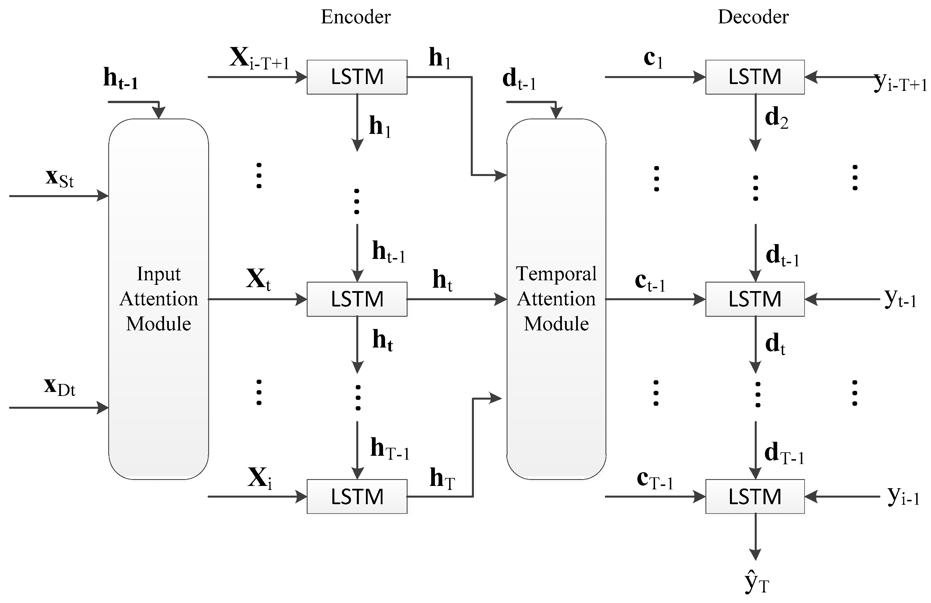
In order to accurately predict bus arrival time, we built a prediction network based on DA-RNN (a dual-stage attention-based recurrent neural network) [18]. The overall prediction framework is shown in Figure 1. The input x_S and x_D are the influencing factors of the arrival time on the last T road segments (including the current road segment). We take the calculation process of ŷ_i as an example to show the internal structure of the prediction network. The calculation processes of ${\widehat{y}}_{(i+1)}$ to ${\widehat{y}}_{(N-1)}$ are similar to that of ŷ_i. The input (y_i-T+1, y_i-T+2…y_i-1) is the travel time on the last T−1 road segments (not including the current road segment). The output ŷ_i is the predicted travel time of the current road segment. The role of the encoder in RNN is to encode the input sequences into a feature representation [20,21]. The encoder with input attention module can adaptively select the relevant influencing factor series. Then we use the LSTM-based decoder to decode the encoded input information. The temporal attention module in the decoder is used to adaptively select relevant encoder hidden states across all time steps. The decoder output predicted travel time ŷ_i. ŷ_i can be calculated by Equation (5). The predicted bus arrival time t_i can be calculated by Equation (9) (k = i).

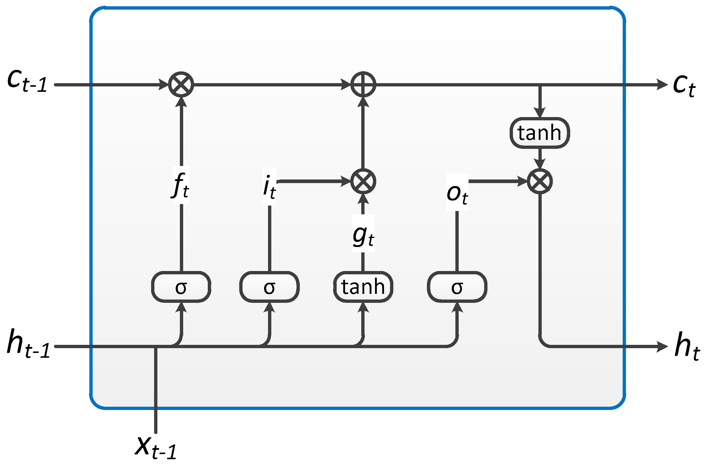
The application of LSTM units can solve the exploding and vanishing gradient problems that are common when training traditional RNNs. The specific structure of LSTM unit is shown in Figure 2. Each unit performs the following operations:

$$i_t=\sigma (W_{ii}{x}_t+b_{ii}+W_{hi}{h}_{t-1}+b_{hi}),$$

(10)

$$f_t=\sigma (W_{if}{x}_t+b_{if}+W_{hf}{h}_{t-1}+b_{hf}),$$

(11)

$$g_t=\tanh (W_{ig}{x}_t+b_{ig}+W_{hg}{h}_{t-1}+b_{hg}),$$

(12)

$$o_t=\sigma (W_{io}{x}_t+b_{io}+W_{ho}{h}_{t-1}+b_{ho}),$$

(13)

$$c_t=f_t\ast c_{t-1}+i_t\ast g_t,$$

(14)

$$h_t=o_t\ast \tanh (c_t),$$

(15)

where h_t is the hidden state at time t, c_t is the cell state at time t, x_t is the input at time t, h_t−1 is the hidden state of the layer at time t−1 or the initial hidden state at time 0, i_t is the input gate, f_t is the forget gate, g_t is the cell gate, o_t is the output gates, σ is the sigmoid function, and * is the Hadamard product.

3.2. Training Procedure

We use minibatch stochastic gradient descent (SGD) together with the Adam optimizer [22] to train the model on a NVidia GeForce RTX 2080 Ti. In order to make full use of the graphic memory and speed up convergence of the model, the size of the minibatch is set to 1024. The learning rate starts from 0.001 and is reduced by 10% after each 10,000 iterations. We implemented the prediction model in the PyTorch framework.

4. Experiments and Discussion

4.1. Data Set

The raw data was provided by Jinan Public Transportation Corporation, Jinan 250100, China. It includes line number, bus identification, station number, arrival time, departure time, length of the road segment, number of intersections, number of lanes, whether the bus lane exists, and the number of passengers. In order to establish the data set, we first cleaned the raw data. Then the arrival time and departure time of each station were converted to the travel time and dwell time.

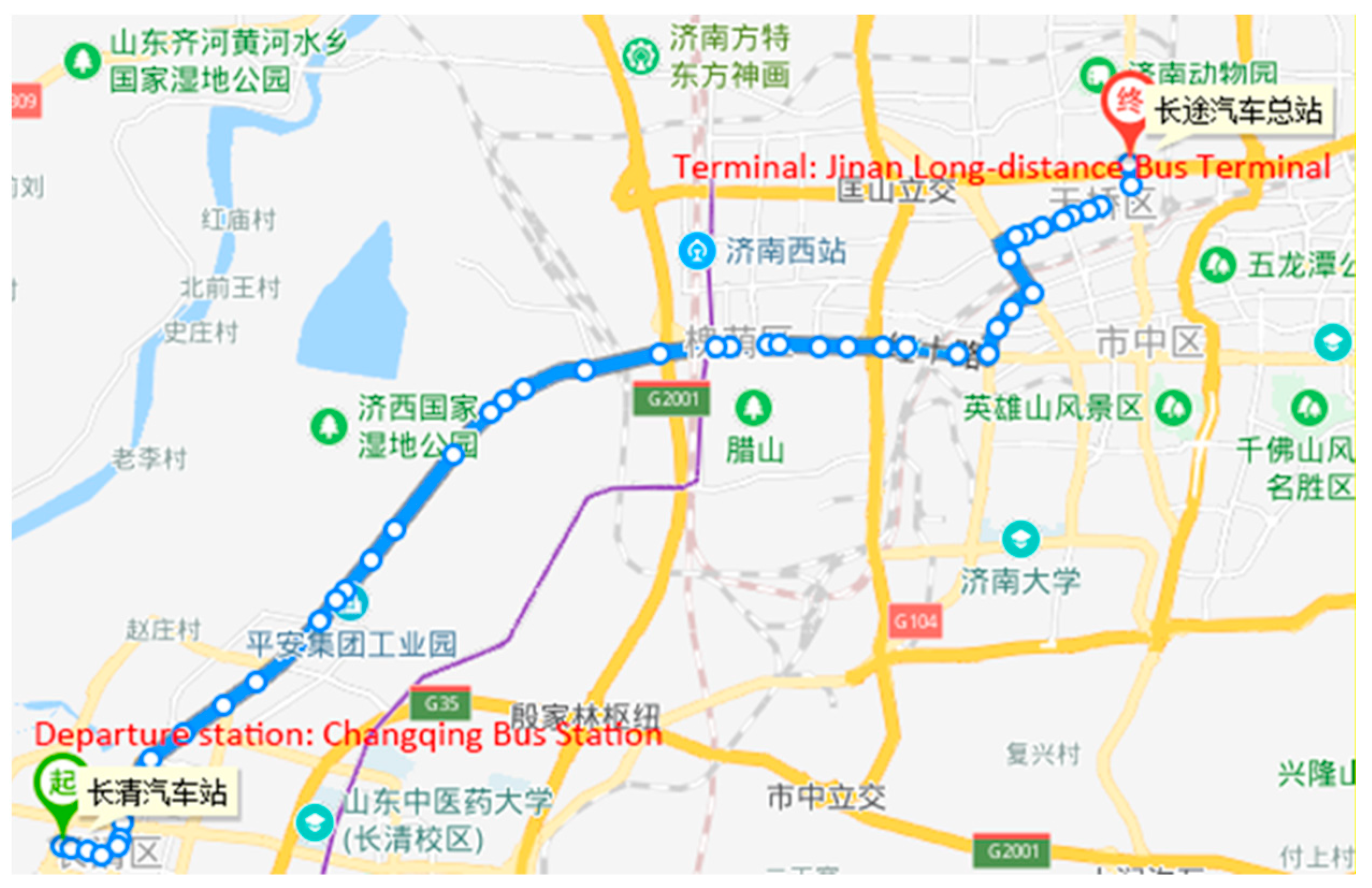
The data set then included the line number, station number, travel time, dwell time, length of the road segment, number of intersections, number of lanes, whether the bus lane exists, and the number of passengers. As shown in Figure 3, there are 50 stations in 1 route, and the route is divided into 49 road segments. We marked the departure station and the terminal in the map because this bus route has not been included in English maps such as Google Maps. The data set contains a total of 2064 run cycles of the bus. We selected the first 1600 cycles as the training set, the middle 200 cycles as the validation set, and the last 264 cycles as the test set.

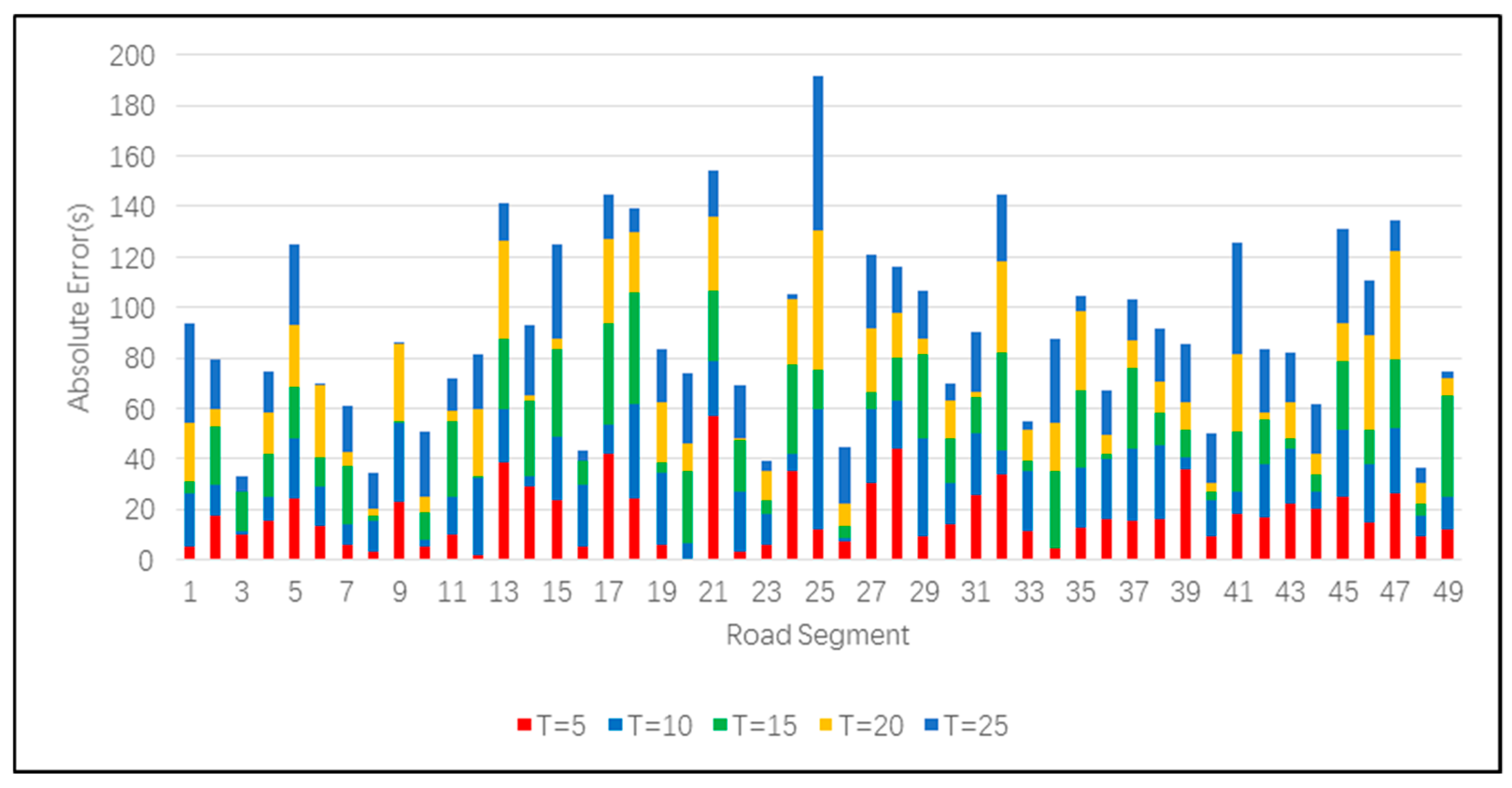
4.2. Parameter Settings and Evaluation Metrics

There are three parameters in the DA-RNN: the number of road segments input each time T, the size of hidden states for the encoder m, and the size of hidden states for the decoder p. The optimization method is grid search. The search range of T is (5, 10, 15, 20, 25). We set m = p for simplicity. The search range of m = p is (16, 32, 64, 128, 256).

The prediction accuracy of bus arrival time t_i can be evaluated by the following metrics.

(1)

Root Mean Squared Error (RMSE):

$$RMSE=\sqrt{\frac{1}{n}{\displaystyle \sum _{i=1}^n{(t_i-{\widehat{t}}_i)}^2}}$$

(16)

(2)

Mean Absolute Error (MAE):

$$MAE=\frac{1}{n}{\displaystyle \sum _{i=1}^n}|t_i-{\widehat{t}}_i|$$

(3)

Mean Absolute Percentage Error (MAPE):

$$MAPE=\frac{1}{n}{\displaystyle \sum _{i=1}^n\left|\frac{t_i-{\widehat{t}}_i}{t_i}\right|}\times 100\%.$$

(18)

4.3. Methods in Comparison Study

4.3.1. LSTM RNN

The main difference between LSTM RNN [17] and DA-RNN is that the former does not have the attention mechanism. LSTM RNN is implemented using the PyTorch framework.

4.3.2. Multilayer Perceptron (MLP)

MLP [16] is a simple neural network composed of fully connected layers [23]. This baseline is a three-layer neural network with 16 neurons per layer.

4.3.3. Kalman Filter

The Kalman filter [1] is an iterative algorithm. Compared to RNN, the Kalman Filter only inputs observation (or prediction if in offline mode) from the previous road segment without storing more data.

4.3.4. SVM

In a bus arrival time prediction task, SVM [4] is used as a regression method. Reference [4] divides the entire bus line into road segments and then predicts the travel time on each segment separately. The optimization of this benchmark is referenced to in the literature [24,25].

4.4. Results

Table 1. Comparisons among different methods used on our dataset.

(a) DA-RNN.
Input Factors	Metrics		T = 5	T = 10		T = 15	T = 20	T = 25
Static factors	RMSE (min)		0.5277	0.5677		0.5293	0.5641	0.5749
	MAE (min)		0.4139	0.4740		0.4344	0.4576	0.4702
	MAPE (%)		17.23%	20.04%		18.11%	19.30%	19.85%
Static &Dynamic factors	RMSE (min)		0.3571	0.3897		0.3643	0.3871	0.3740
	MAE (min)		0.2815	0.3257		0.2966	0.3114	0.3085
	MAPE (%)		11.81%	13.76%		12.19%	13.30%	13.06%
(b) LSTM RNN.
Metrics		Static Factors			Static &Dynamic Factors
RMSE (min)		0.6670			0.5261
MAE (min)		0.5229			0.4258
MAPE (%)		22.32%			19.07%
(c) MLP.
Metrics		Static Factors			Static &Dynamic Factors
RMSE (min)		0.8240			0.6908
MAE (min)		0.6711			0.5623
MAPE (%)		28.77%			23.85%
(d) Kalman Filter.
Metrics		Static Factors			Static &Dynamic Factors
RMSE (min)		1.397			1.278
MAE (min)		1.065			0.9851
MAPE (%)		71.04%			63.26%
(e) SVM.
Metrics		Static Factors			Static &Dynamic Factors
RMSE (min)		1.129			0.9718
MAE (min)		0.8716			0.7663
MAPE (%)		52.39%			38.03%

is a summary of the experimental results. According to the three evaluation indexes of RMSE, MAE and MAPE, DA-RNN achieves the best prediction accuracy. Regardless of the method used, the accuracy of the prediction can always be improved by inputting dynamic factors. The optimal value of the parameter T is 5, while the optimal values of the parameters m and p are both 128. This is because the influence of the values of m and p on the prediction is small relative to T, and they are structural parameters of the RNN without any clear physical meaning. Taking into account the length of this article, Table 1 only lists the experimental results when m = p = 128.

To more visually demonstrate the experimental results, we plotted Figure 4 and Figure 5 based on the labels in the test set and their predicted values.

In Section 2, we not only used the calculation formula of the next station arrival time t_i, but also the calculation formula of the remaining station arrival time t_i+1 to t_k. If the bus is located on the i-th road segment, then the dynamic factors of the (i+1)-th to k-th road segment are unknown. So t_i+1 to t_k can only be predicted with a static model. First enter t_i into the static model to get t_i+1. Then enter t_i into the static model to get t_i+1. We performed iterative operations until t_k was obtained. The result under offline conditions is shown in Figure 6.

4.5. Discussion

4.5.1. The Influence of Dynamic Factors

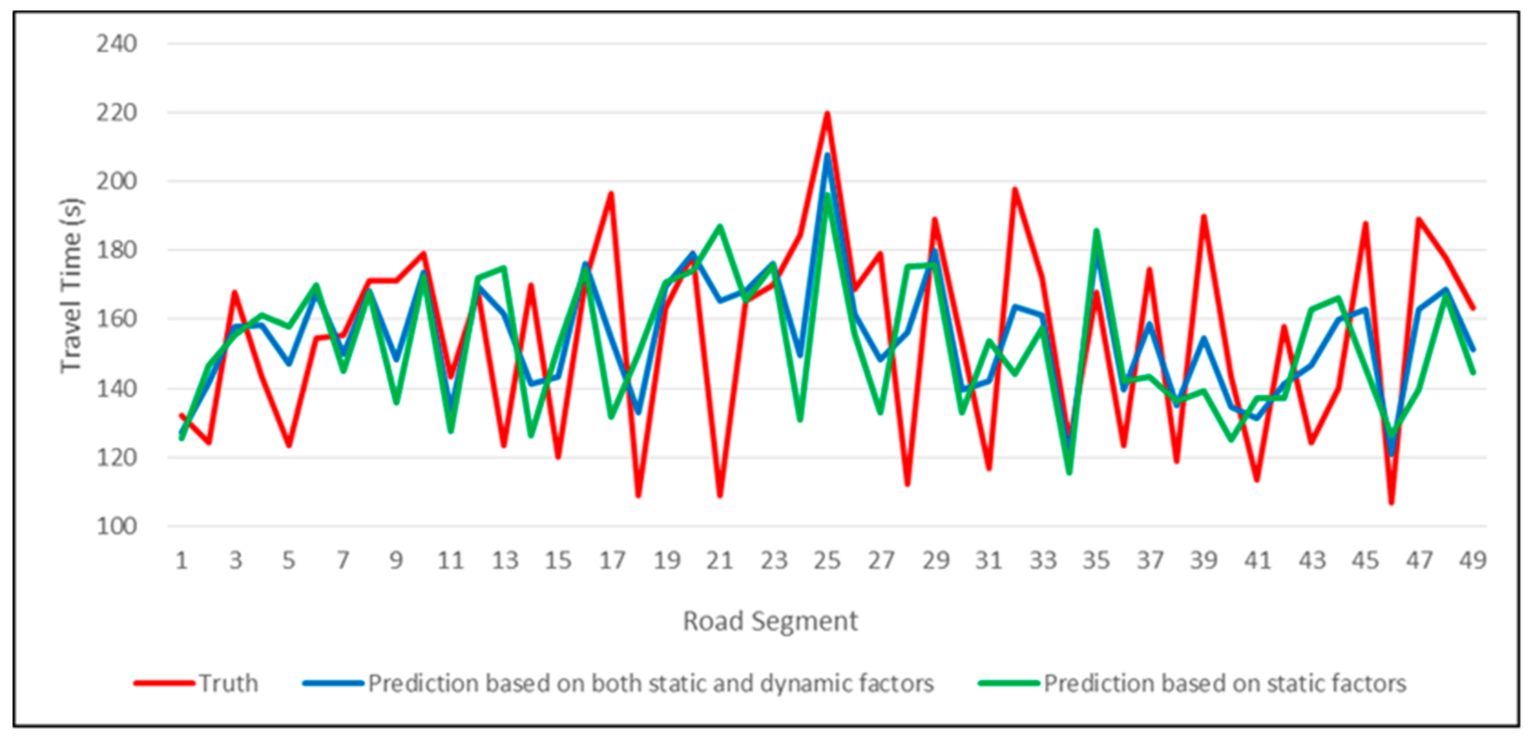
Experiments show that regardless of the method used, considering dynamic factors is always beneficial to improve prediction accuracy. Dynamic information reflects changes in bus operation and is more time-sensitive than static information. Figure 4 shows the comparison of the true and predicted values of a sequence extracted in the test set. For a certain bus, the model prediction results using only static factors are more closely inclined to the historical average. When the actual situation is significantly different from the average of the previous observations, this static model will get unsatisfactory prediction results. Proper use of dynamic factors can alleviate this problem.

4.5.2. The Necessity of Long-Term Dependencies

As shown in Table 1, regardless of whether dynamic factors are used, RNN’s prediction of bus arrival time is significantly better than that of other methods. This is because RNN can learn long-term dependencies, while other algorithms in the experiments only build short-term dependencies. Both DA-RNN and LSTM RNN contain the LSTM structure. The LSTM units can selectively “forget” old information, “remember” new information and determine output. So the RNN-based models can make full use of the information of the last several road segments, while other methods only use the information of the current road segment for prediction. In other words, all methods establish a mapping relationship from influencing factors to travel time. The difference is that the mapping relationship of other models exists only in a single road segment, while the RNN-based model can establish a mapping relationship in several road segments. Effective use of historical information is the reason why the RNN network can get better prediction results.

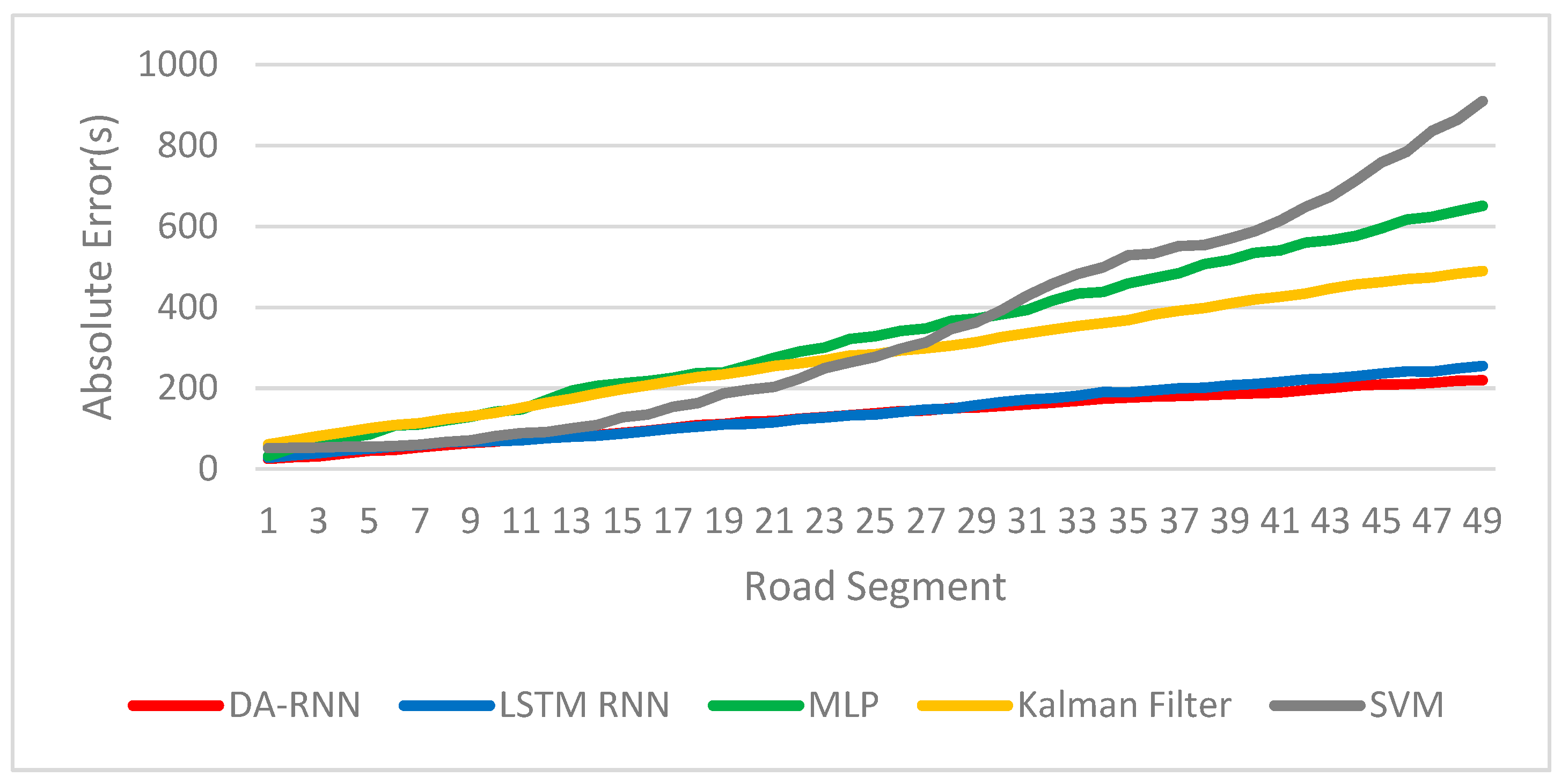
Figure 6 shows that in offline mode, the MAE of the prediction results increase with the increase of the number of stations. Among them, the MAE of two RNN models is small and the growth rate is slow. The main reason for the growth of MAE is that the arrival time was not added, and the prediction result cannot be corrected according to the observations, so the absolute error of the prediction was accumulated in the iteration. The secondary reason is that dynamic factors cannot be utilized under offline conditions. In offline mode, RNN models exhibits greater robustness. This indicates that long-term dependency is indispensable in the bus arrival time prediction task. It is worth noting that the prediction MAE at the 10th station of the proposed RNN model can still be kept within one minute (59.41 s). This proves that our approach also has high practical value in the offline state.

4.5.3. Why Attention Mechanism Is Needed?

Based on the experimental results, DA-RNN always outperforms LSTM RNN in both online and offline conditions. To find the reason why this occurs, we must start with the structure of the neural network. Compared with LSTM RNN, DA-RNN has two attention modules. The input attention module adaptively extract the relevant driving factors. This is why the difference in performance between the two RNNs will be widened after the dynamic factors are input. As shown in Figure 6, in off-line mode, the performance gap between DA-RNN and LSTM RNN is not obvious when the number of stations is small, and the difference between the two is significantly increased when the number of stations is greater than 35. This is because the temporal attention module can select relevant encoder hidden states across all time steps. DA-RNN has a stronger ability to capture long-term dependencies. In order to improve the prediction accuracy, it is necessary to input more static and dynamic factors into the model, and to increase the ability to learn long-term dependencies. The rational use of the attention mechanism is crucial to improving the accuracy of prediction.

5. Conclusions

Accurate prediction of bus arrival times is an important issue in the field of smart transportation, and it is also a challenging problem. Most of the existing solutions are based on static information, such as the number of stations, the spacing of adjacent stations, and the number of intersections on each road segment. These static data collection costs are low (which can be obtained directly from Google Maps if the information is correct). These methods have guiding significance for the planning of bus routes, but their prediction accuracy has not yet met the more sensitive traveling time requirements such as estimated waiting time and real-time bus scheduling.

In this paper, we improved the prediction accuracy by inputting dynamic factors. In addition to the methods in the experiment, this method of improving the prediction accuracy can theoretically be applied to other methods. The experimental results show that the ability to learn long-term dependencies is the main reason for RNN to gain an advantage in the prediction task. From the perspective of extracting the dominant factors and improving the learning ability for long-term dependency, the attention mechanism is crucial for prediction.

In the future, we aim to develop this approach further by incorporating more heterogeneous dynamic factors, such as weather, road congestion, traffic signal status, etc. Moreover, considering the interactions between multiple bus lines, the influence of the connection relationship between the stations in the public transportation network on bus arrival times is an interesting research direction.

References

- Jisha, R.C.; Jyothindranath, A.; Sajitha Kumary, L. IoT based school bus tracking and arrival time prediction. In Proceedings of the International Conference on Advances in Computing, Communications and Informatics (ICACCI), Udupi, India, 13–16 September 2017; pp. 509–514. [Google Scholar]
- Achar, A.; Bharathi, D.; Kumar, B.A.; Vanajakshi, L. Bus Arrival Time Prediction: A Spatial Kalman Filter Approach. IEEE Trans. Intell. Transp. Syst. 2019, 1–10. [Google Scholar] [CrossRef]
- Kumar, B.A.; Vanajakshi, L.; Subramanian, S.C. Bus travel time prediction using a time-space discretization approach. Transp. Res. Part C Emerg. Technol. 2017, 79, 308–332. [Google Scholar] [CrossRef]
- Yu, B.; Lam, W.H.K.; Tam, M.L. Bus arrival time prediction at bus stop with multiple routes. Transp. Res. Part C Emerg. Technol. 2011, 19, 1157–1170. [Google Scholar] [CrossRef]
- Yang, M.; Chen, C.; Wang, L.; Yan, X.; Zhou, L. Bus arrival time prediction using support vector machine with genetic algorithm. Neural Netw. World 2016, 26, 205–217. [Google Scholar] [CrossRef]
- Bai, C.; Peng, Z.R.; Lu, Q.C.; Sun, J. Dynamic bus travel time prediction models on road with multiple bus routes. Comput. Intell. Neurosci. 2015, 2015, 63. [Google Scholar] [CrossRef] [PubMed]
- Yin, T.; Zhong, G.; Zhang, J.; He, S.; Ran, B. A prediction model of bus arrival time at stops with multi-routes. Transp. Res. Procedia 2017, 25, 4623–4636. [Google Scholar] [CrossRef]
- Liu, W.; Liu, J.; Jiang, H.; Xu, B.; Lin, H.; Jiang, G.; Xing, J. WiLocator: WiFi-Sensing Based Real-Time Bus Tracking and Arrival Time Prediction in Urban Environments. In Proceedings of the IEEE 36th International Conference on Distributed Computing Systems (ICDCS), Nara, Japan, 27–30 June 2016; pp. 529–538. [Google Scholar]
- Yu, H.; Wu, Z.; Chen, D.; Ma, X. Probabilistic Prediction of Bus Headway Using Relevance Vector Machine Regression. IEEE Trans. Intell. Transp. Syst. 2017, 18, 1772–1781. [Google Scholar] [CrossRef]
- Xu, H.; Ying, J. Bus arrival time prediction with real-time and historic data. Cluster Comput. 2017, 20, 3099–3106. [Google Scholar] [CrossRef]
- Gal, A.; Mandelbaum, A.; Schnitzler, F.; Senderovich, A.; Weidlich, M. Traveling time prediction in scheduled transportation with journey segments. Inf. Syst. 2017, 64, 266–280. [Google Scholar] [CrossRef]
- Yu, B.; Wang, H.; Shan, W.; Yao, B. Prediction of Bus Travel Time Using Random Forests Based on Near Neighbors. Comput. Aided Civ. Infrastruct. Eng. 2018, 33, 333–350. [Google Scholar] [CrossRef]
- Nabavi-Pelesaraei, A.; Rafiee, S.; Mohtasebi, S.S.; Hosseinzadeh-Bandbafha, H.; Chau, K. Integration of artificial intelligence methods and life cycle assessment to predict energy output and environmental impacts of paddy production. Sci. Total Environ. 2018, 631, 1279–1294. [Google Scholar] [CrossRef] [PubMed]
- Fotovatikhah, F.; Herrera, M.; Shamshirband, S.; Chau, K.W.; Ardabili, S.F.; Piran, M.J. Survey of computational intelligence as basis to big flood management: Challenges, research directions and future work. Eng. Appl. Comput. Fluid Mech. 2018, 12, 411–437. [Google Scholar] [CrossRef]
- Kaab, A.; Sharifi, M.; Mobli, H.; Nabavi-Pelesaraei, A.; Chau, K. Combined life cycle assessment and artificial intelligence for prediction of output energy and environmental impacts of sugarcane production. Sci. Total Environ. 2019, 664, 1005–1019. [Google Scholar] [CrossRef] [PubMed]
- Gurmu, Z.K.; Fan, W.D. Artificial neural network travel time prediction model for buses using only GPS data. J. Public Transp. 2014, 17, 45–65. [Google Scholar] [CrossRef]
- Pang, J.; Huang, J.; Du, Y.; Yu, H.; Huang, Q.; Yin, B. Learning to Predict Bus Arrival Time From Heterogeneous Measurements via Recurrent Neural Network. IEEE Trans. Intell. Transp. Syst. 2019, 20, 3283–3293. [Google Scholar] [CrossRef]
- Qin, Y.; Song, D.; Cheng, H.; Cheng, W.; Jiang, G.; Cottrell, G.W. A dual-stage attention-based recurrent neural network for time series prediction. In Proceedings of the Twenty-Sixth International Joint Conference on Artificial Intelligence (IJCAI-17), Melbourne, Australia, 19–25 August 2017; pp. 2627–2633. [Google Scholar]
- Dong, P.; Li, D.; Xing, J.; Duan, H.; Wu, Y. A Method of Bus Network Optimization Based on Complex Network and Beidou Vehicle Location. Futur. Internet 2019, 11, 97. [Google Scholar] [CrossRef]
- Cho, K.; van Merrienboer, B.; Bahdanau, D.; Bengio, Y. On the Properties of Neural Machine Translation: Encoder–Decoder Approaches. arXiv 2014, arXiv:1409.1259. [Google Scholar]
- Cho, K.; Van Merriënboer, B.; Gulcehre, C.; Bahdanau, D.; Bougares, F.; Schwenk, H.; Bengio, Y. Learning phrase representations using RNN encoder-decoder for statistical machine translation. arXiv 2014, arXiv:1406.1078. [Google Scholar]
- Kingma, D.P.; Ba, J. Adam: A Method for Stochastic Optimization. arXiv 2014, arXiv:1412.6980. [Google Scholar]
- Najafi, B.; Faizollahzadeh Ardabili, S.; Shamshirband, S.; Chau, K.W.; Rabczuk, T. Application of anns, anfis and rsm to estimating and optimizing the parameters that affect the yield and cost of biodiesel production. Eng. Appl. Comput. Fluid Mech. 2018, 12, 611–624. [Google Scholar] [CrossRef]
- Moazenzadeh, R.; Mohammadi, B.; Shamshirband, S.; Chau, K.W. Coupling a firefly algorithm with support vector regression to predict evaporation in northern Iran. Eng. Appl. Comput. Fluid Mech. 2018, 12, 584–597. [Google Scholar] [CrossRef]
- Yaseen, Z.M.; Sulaiman, S.O.; Deo, R.C.; Chau, K.W. An enhanced extreme learning machine model for river flow forecasting: State-of-the-art, practical applications in water resource engineering area and future research direction. J. Hydrol. 2018, 569, 387–408. [Google Scholar] [CrossRef]
© 2019 by the authors. Licensee MDPI, Basel, Switzerland. This article is an open access article distributed under the terms and conditions of the Creative Commons Attribution (CC BY) license (http://creativecommons.org/licenses/by/4.0/).