Abstract
E-commerce is becoming more and more the main instrument for selling goods to the mass market. This led to a growing interest in algorithms and techniques able to predict products future prices, since they allow us to define smart systems able to improve the quality of life by suggesting more affordable goods and services. The joint use of time series, reputation and sentiment analysis clearly represents one important approach to this research issue. In this paper we present Price Probe, a suite of software tools developed to perform forecasting on products’ prices. Its primary aim is to predict the future price trend of products generating a customized forecast through the exploitation of autoregressive integrated moving average (ARIMA) model. We experimented the effectiveness of the proposed approach on one of the biggest E-commerce infrastructure in the world: Amazon. We used specific APIs and dedicated crawlers to extract and collect information about products and their related prices over time and, moreover, we extracted information from social media and Google Trends that we used as exogenous features for the ARIMA model. We fine-estimated ARIMA’s parameters and tried the different combinations of the exogenous features and noticed through experimental analysis that the presence of Google Trends information significantly improved the predictions.
1. Introduction
E-Shops are recently gaining more and more popularity among users. Amazon (https://www.amazon.com/), Ebay (https://www.ebay.com/), Tesco (https://www.tesco.com/groceries/?icid=dchp_groceriesshopgroceries) and others, are huge companies which sell any kind of products owing therefore most of their success to online purchases, home delivery and low prices that they can offer.
In the past ten years, Amazon had an impressive growth that allowed building its own delivery and data centers across the world in order to serve its users in the best possible way. The main reasons for Amazon’s success is due to the amount of different products sold along with its customer care, its advertisings, the respect and trust gained among users during the past years and, especially, products’ prices. Without a doubt, Amazon has today become the number one online retailer for many consumers. According to Morgan Stanley, Amazon’s cloud arm AWS (https://aws.amazon.com), prime subscriptions, and advertising segment, greatly helped to make Amazon a 1 trillion company in 2018. Therefore, there is a lot of research related to Amazon services and price forecasting of Amazon products is one direction where many researchers are headed.
Research has also brought to light new commercial services such as CamelCamelCamel (https://camelcamelcamel.com) that earns from just showing a product’s trend over time. CamelCamelCamel tracks every product’s price trend over time on different marketplaces. For each product, it compares its trend history on each marketplace and alerts the interested user in a certain product when its price gets lower than its average value or under a given chosen threshold. It tracks marketplaces like Amazon and Google Shopping.
The prices of the products Amazon sells are influenced by several factors, most of which are unknown. They can be influenced by inflation, by the amount of sales, by its popularity, by the popularity of its manufacturer, by the popularity of its category, by the users reviews, by the holiday periods and so on. Some of the information related to the products are unknown, such as the number of their sales, since Amazon does not disclose this kind of data for strategic reasons. On the other hand, some of the Amazon data related to its products can be gathered using Amazon APIs or can be extracted using crawlers, scrapers and other techniques.
The goal of our work was to study and analyze how the historical information and external factors might influence the future price trend of a given product and the impact of each of the external factors on the forecast of the price of each product. We have used Amazon as platform to extract unstructured products information and prices with the objective to perform the forecast of Amazon products’ prices on data extracted with Amazon APIs and crawlers to understand whether external information, such as those provided by Google Trends or customer reviews (the latter has already been verified bringing effects on future product pricing and demand [1]), might bring benefits to the overall prediction.
We have represented the extracted data in form of time series and decided to use ARIMA (Autoregressive Integrated Moving Average) for the forecast step. Out of all machine learning and statistical methods that can be used for financial time series forecasting highlighted by the authors in [2,3], the choice of using ARIMA depends on the fact that it is well suited for the data types we have collected and allows working with exogenous variables, which consist of further data we can feed to the model. A lot of the data we have extracted related to the Amazon products’ prices over a wide interval time exhibit consistent pattern over time with a minimum amount of outliers. Basically, the first thing we have analysed has been the stationarity of the data and we have noticed that most of the prices of a given product remain at a fairly constant level over time. This happens for a lot of products. There are also cases of non stationarity time series in our data and this is where we had to perform some preprocessing steps. Our method can be applied to any kind of product as long as we provide the price and the related date. ARIMA also works well in presence of several missing daily tuples (price, date) among its inputs and that is also one more reason we chose it (as we had missing data for certain products in certain interval times). Of course, the higher the number of entries per each product, the more precise the forecast step will be.
Similar studies using ARIMA for price forecasting have been done in [4,5,6,7,8,9,10,11]. Other works focused on the forecasting of e-commerce prices have been proposed in [12] where authors proposed LSTM neural networks to obtain better prediction performances in daily phone prices in one particular marketplace, amazon.fr. In one further work [13], researchers adopted a Stochastic Differential Equations (SDE) approach to describe a plausible course of the online auction price. The proposed model has several practical implications. First, an SDE model enables one to individually model an online auction price curve in which the price dynamics can be determined by its own parameters. Second, this approach facilitates the price prediction of an online auction, which can help improving auction strategies.
Besides, several articles have used Google Trends to improve the forecasts of different phenomena [14,15]. We have trained the ARIMA model with 90% of the data we collected and predicted the prices of the remaining data. We had to fine-estimate the ARIMA parameters and performed the forecast with a low Mean Absolute Percentage Error Score. ARIMA depends on different inputs such as ACF (AutoCorrelation Function) and PACF (Partial AutoCorrelation Function) and, on the basis of the time series theory [16], it works well if the process is stationary. For this reason, when it is non-stationary we introduce a preprocessing step.
It should be observed that several studies in literature proved that many machine learning models are able to get the same performance of ARIMA (i.e., in terms of forecasting performance) when they involved a large number of time series [17,18]. We have chosen to exploit ARIMA models instead of other machine learning ones for the following reasons: (i) differently from many machine learning approaches, they provide good forecasting performance when a small/big number of data (i.e., time series) is employed; (ii) in terms of short-run forecasting those models are relatively more robust and efficient than more complex ones [19]; (iii) the strictly statistical method used by ARIMA only requires the prior data of a time series in order to generalize the forecast, then it is able to increase its forecasting accuracy by involving a minimum number of parameters [20].
More in detail, the scientific contribution of this paper is the following:
- First, this is the first work analyzing the correlation of Google Trends and products reviews information with Amazon products’ prices, using huge amount of real world data. We have developed crawlers that extracted about 9 millions of products and 96 millions of tuples with information related to their prices, their manufacturers, categories they belong, Google Trends, and reviews.
- Second, a deep analysis of how Google Trends information improved the forecast task when used as exogenous variable within our ARIMA model is performed;
- Finally, we developed and made available an open source framework which allows downloading and crawling of Amazon products information and the tuning and employment of the ARIMA model.
- Last but not least, we built a database of a huge collection of Amazon products, their reviews, their price over time and the related Google Trends information.
The rest of our paper is organized as follows. Section 2 presents some related works on the price forecasting and the statistical tools and classifiers used for such a purpose. Section 3 details the data we have used for our experiment. Section 4 describes Price Probe: how the data have been collected and the suites of crawler we have developed for such a purpose. Section 5 describes the used methodology and how we set the configuration parameters of the ARIMA model. Results we have obtained which include a detailed performance evaluation are discussed in Section 6 whereas Section 7 ends the paper with final remarks and directions where we are headed.
2. Related Work
Several researchers have employed ARIMA models for forecast of stock prices. As an example, authors in [4,8] describe as ARIMA can easily handle such a data format and how it is well suited for time series forecasting. One more example is represented by [21] where authors described an ARIMA model with currency as exogenous feature used to forecast commodity prices. ARIMA has also been employed within the agriculture domain where authors in [6] discussed how they have employed it for forecasting crop prices, and results indicate very low error values in terms of MSE (Mean Squared Error) and MAPE (Mean Absolute Percentage Error). Within the same domain, one more work is represented by [7], where authors described how to employ ARIMA for forecast cloud coverage based on ground-based cloud images. In particular, taking into account the correlation about cloud coverage over time, authors obtained an approximate error of 8% of the predictions compared to real values.
Energy is one more domain of application for ARIMA. For example, work in [5] describes an ARIMA model for forecasting electricity price during weeks, having as input wavelet transform applied to time series related to electricity prices. The application of wavelet transform further reduces the error of predictions performed by the model. In a similar way, other works related to the forecast of energy have been discussed in [9], where the authors described an ARIMA model for forecast coal’s consumption in China, and in [10] where authors used it to forecast energy consumption of Turkey. One more example can be found in [11] where authors describe the use of exogenous variables for residential low voltage distribution networks.
It should be observed that, regardless the adopted model, when exogenous variables are not used, there is a limit of predictability [18], whereas the appropriate selection of such variables leads towards an improvement of the forecasting performance [22].
In literature, researchers have already tried to include values returned by Google Trends as exogenous variables in ARIMA models for forecasting of oil consumption [23]. Also, authors in [24] described an ARIMA model using Google Trends modified with Twitter’s sentiment score to estimate consumption and sales for a particular business. In fact, Sentiment Analysis is one more domain where ARIMA models have been employed. Moreover, authors in [25] have used sentiment analysis of products users reviews in a time interval to build an ARIMA model to predict the amount of sales of the products. Moreover, authors in [26] focused on forecasting the price of house property and electronic products using sentiment news from Baidu, a well-known portal website in China analysing news content and extracting key events related to the products. Results indicate that predicted prices of products can be influenced by sentiment factors. Similarly, authors in [27], based on the user comments data from a popular professional social networking site of China stock market called Xueqiu, calculated the investor sentiment of each stock and performed their analysis based on the Thermal Optimal Path method. The results show that the sentiment data was not always leading over stock market price but it might be used to predict the stock price only when the stock had high investor attention.
Several works have tried to address the concept of stationarity, and seasonality of the input data of an ARIMA model. More in general, authors in [28] described how the problem of time series forecasting should be approached, focusing on the importance, for the forecasting, to remove trends or seasonality of the considered time series. To check whether a given time series is stationary or not, authors in [29] introduced the Adfuller Test. They also provided information related to the meaning of stationary series, when they can be considered good for statistics analysis and prediction or not. Similarly, authors in [30] described the Augmented Adfuller Test and discussed more deeply the concept of stationarity of time series and how the choice of ARIMA’s parameter d is bound to the stationarity of the time series. On top of that Ng and Perron in [31] introduced a modified unit root test showing and proving that it was more powerful and reliable than the ADF test. Other works focused on the tuning and the correct choice of the parameters needed for an ARIMA model to work. In particular, authors in [32] described Box and Jenkins, a method used to calculate ARIMA’s input parameters (p, q, d). This resource deeply explores and describes how to find (p, q, d), what they are and what their value means. Another example is constituted by [33] where authors described ACF, PACF and other techniques used in ARIMA. The authors in [34] described a python library employed to find PACF and ACF values for a time series in order to detect, respectively, ARIMA’s p and q parameters. In this paper we used much of the techniques introduced within this section. Our choice of using ARIMA as best model for forecasting of products’ price is in line with the findings of previous work in literature and also supported by the work of researchers that have compared the performances of ARIMA models with ARMA (autoregressive-moving-average) models [35] and showed how the former has lower error and higher accuracy.
Other recent work investigated whether measurements of collective emotional states derived from large scale networks feeds are correlated with stock transaction data over time [36].
3. Data Description
In this section, we are going to detail the data used in this paper. Our data are stored in different PostgreSQL tables reported as follows (please contact the authors if interested in obtaining the data).
- Products—which contains main information on the Amazon products;
- Manufacturers—which contains information about the manufacturers;
- Categories—which contains information about the categories of the products;
- Categories products—which contains the associations between products and categories;
- Prices—which contains information about the prices of the Amazon products;
- reviews—which contains information about the reviews of the products.
- trends—which contains information about Google Trends on the manufacturers of the Amazon products;
Figure 1 shows the tables mentioned above with their related fields and relations. The process of extraction of all the data is detailed in Section 4.1 and Section 4.2.
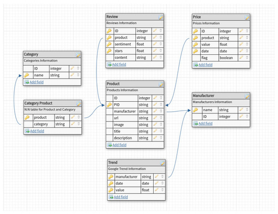
Figure 1.
Data tables and their relationships.
3.1. Products
The table related to the products stores different information about each Amazon product. The table includes an id, the manufacturer of the given product, the product’s URL, the product’s title that appears on Amazon and the URL of its related image.
3.2. Manufacturers
This table stores the name related to the manufacturers of each product. This table has also been employed to fetch Google Trends entries. For each manufacturer we extracted it Google Trends history. We collected this information because we wanted to understand whether external data such Google Trends might affect our forecast.
3.3. Categories
This table stores the name of each category. In particular, we stored categories of each product. Each product can be associated with one or more categories. The rationale behind having the categories was to test whether the forecast process was more precise for products of the same categories.
3.4. Categories Products
This table stores the associations (product, category) as each product may have multiple categories and, vice-versa, each category can be assigned to several products.
3.5. Prices
This table contains all the information about the prices of each product over time. We have about 9 millions of different products and about 90 millions of different prices taken within the interval time from 2015 to 2016. Prices information are expressed in tuples (item, price, date). Each of such a tuple is unique and, therefore, a given product has one price information in a given day. Certain products have daily entries in consecutive days, others have not.
3.6. Reviews
This table stores information about reviews of products. Each element includes the product that the review is referred to, a description of the review, the date when the review has been posted, an integer number between −1 and +1 that corresponds to the sentiment on that product and a star field including a vote expressed as several stars between 0 and 5. Not all the products have reviews. If they have, they might have one or more reviews per day. The content of a given review includes a comment posted by a user. We have collected this information because we wanted to understand whether the reviews had an influence and could bring benefits for the forecast of the products’ prices. The domain of Sentiment Analysis related to the reviews might be a bit tricky as more experienced users might influence future users reviews on a same product or a user review might also be influenced by the popularity of the underlying product’s manufacturer and the category maturity [37,38,39]. We followed the same direction of a similar work that employed ARIMA within the Sentiment Analysis domain [25] to understand whether or not a product would have success. For instance, we thought that many negative reviews in terms of stars and sentiment score could lead to a price decrease; this has been validated and highlighted by works such as [40] where authors stated that e-commerce success might take decisions based on the social influence of its users.
3.7. Trends
This table stores information about trends that we extracted using Google Trends for each manufacturer of the products we collected over time. A value between 0 and 100 expressed the trend’s value where 100 indicates a strong trend whereas 0 indicates a weak trend on the given product and date. For each manufacturer we extracted a Google Trends entry. Essentially, we have a manufacturer popularity expressed as a pair (value, date). The idea was to collect this kind of data to understand how the popularity of a given manufacturer might affect the forecast step. A similar work has been conducted in [23] where authors employed Google Trend as a feature in ARIMA. Section 4.2 describes in detail how we have extracted Google Trend information for each manufacturer.
4. Price Probe
Our RESTful back-end of Price Probe collects and stores all the data in a relational database so that it is easy to prepare queries for the forecast of an item. Our system is flexible enough and allows collecting any sort of new external features: it is straightforward to extend our back-end functionalities by adding new modules and REST (REpresentational State Transfer) handlers to it. Moreover, our crawlers and tools are all small and independent microservices which share a common configuration: anyone willing to develop a new crawler can extend the current pipeline and define which features he/she wants to collect. The suite of software we have developed is easily deployable using Docker-Compose (https://docs.docker.com/compose/).
The data used in our study have been collected using the APIs of Amazon and ad-hoc crawlers we have developed within our suite of software that we propose. As such, this section describes the suite of crawlers we have developed to extract, collect and process the data mentioned in Section 3 in form of time series. Our crawlers are independent microservices that extract data calling external APIs and services, processing the resulting information and adding it to our collection via REST calls to our back-end. Our back-end has been written in Google’s Golang (https://golang.org/) and is available for free download (https://github.com/AndreaM16/go-storm). Figure 2 shows the architecture of our crawling system.
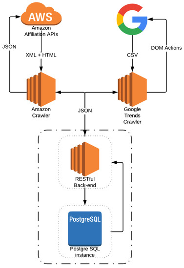
Figure 2.
Crawling Suite Architecture.
In the following, we will describe the data we have crawled from Amazon and Google Trends. In particular, Section 4.1 covers the Amazon’s data collecting process whereas Section 4.2 describes the Google Trends data collecting process.
4.1. Amazon
As stated in Section 3, originally, for each product we had only (price, date) tuples for a total of about 90M unique tuples. These data have been crawled using Amazon Affiliation APIs (https://docs.aws.amazon.com/AWSECommerceService/latest/GSG/GettingStarted.html). On a daily basis, our crawlers collected the information about products and prices available on Amazon. The time interval when we had run our crawlers and collected our data was between 2015 and 2016. This collection had several issues. Prices were represented in different formats (text, double, uint, ...) and a pre-processing step was necessary. Using different tools such as AWK, we were able to parse these heterogeneous data to a common format. For simplicity, we also formatted all the date entries. After that, we uploaded the results to a PostgreSQL database. Additional data such as manufacturers and reviews have been gathered by developing a microservice that performs API calls to Amazon using Amazon Affiliation APIs. Such a microservice is freely available on a GitHub repository (https://github.com/AndreaM16/go-amazon-itemlookup). These APIs expose XML bodies describing a given product. This body contains different parameters such as product’s manufacturer, categories, reviews page URL and so on. Unluckily, APIs do not expose any kind of information about the reviews but only a URL that provides an HTML page containing paginated reviews. It was necessary to scrape this page to get reviews in form of content, stars and date. We found out that for some products, APIs do not return any useful information. Therefore, for some products it was impossible to fetch their manufacturer or reviews. The Polarized Sentiment Analysis was performed on product’s content using Vader Sentiment Analysis (https://github.com/cjhutto/vaderSentiment) and referenced here [41]. Concerning the reviews, as stated in Section 3.6, per each product, we found up to n reviews (sometimes even zero). This was an issue when aggregating the data as performing a join between the tuples (item, date, price) and (item, date, sentiment, stars), might have 0 or very few rows. Thus, in order to have a more consistent number of reviews having at least one entry per day when joining the prices data, we did the following. We wrote a small tool, available online (https://github.com/AndreaM16/review-analyzer), that generated a list of unique daily reviews. If a certain day had more than one review, we calculated an average of their Sentiment and Stars and inserting that in . These Sentiment and Stars values were calculated following the formula:
where and are the averaged values obtained as new Sentiment and Stars values for the resulting review that will be inserted in the daily reviews list and related to . is a list of consecutive days reviews so that . On top of that, we managed to fill the missing entries between two reviews belonging to by making the average of the two related entries, and .
The resulting review is inserted into a final list of daily consecutive reviews where . In this way, we had a unique review for each date within the range that goes from the very first to the very last date of a given product. The reader notices that it still might be possible for a given product to have a time series of (date, price) tuples with some missing entries (missing values for some day of the reference interval time). The missing reviews have been computed when for a given product we had (date, price) tuples information but not its related review.
4.2. Google Trends
Google Trends data tracks the popularity of a manufacturer over time. Starting from manufacturers, we fetched their Google Trends history from 2015 to the middle of 2016. To do so, we built a crawler using Selenium Webdriver (http://www.seleniumhq.org/projects/webdriver/) in Python and Golang that for a given manufacturer, looked for its trend, downloaded its csv data, parsed and posted it to our back-end. We had to use Selenium because Google Trends does not have open APIs to get a given text input’s popularity. Moreover, the downloaded csv file contained only weekly (value, date) entries, hence, one entry per week. Since we needed external data to be in daily format (as stated in Section 4.1), we had to process it and get an entry for each missing day. This has been achieved by using the same approach used to fill the missing reviews. Given two consecutive date trend entries and belonging to , so that, for each of them, , we get the missing days values (e.g., for ) by calculating the average of and . The reader notices that the approach we have employed to solve missing values has been taken from [42]. As the number of missing values (both for Google Trends information and reviews) were less than 2% for each time series on each considered Amazon product, we did not include any sensitivity analysis. We limited to report for completeness the method we have employed to fill missing values.
The resulting trend entry is inserted into a final list of daily trend entries where . In this way, we had a unique trend entry for each date in the interval range of a given product. The result has been posted as the reputation over time of a given manufacturer in our back-end. Similarly as for the reviews, the missing Google Trends information have been computed when, for a given product, we had (date, price) tuples information but not Google Trends. The Selenium + Python code we developed is freely available at the following GitHub repository (https://github.com/AndreaM16/yaggts-selenium). The code simply takes a text as input, for instance Apple, and downloads a csv file containing its related weekly formatted entries. The Golang code (https://github.com/AndreaM16/yaggts) calls the Python code sending an input text, and waiting for the csv to be downloaded, parsed and processed as stated above. Results are then posted to our back-end.
5. Our Approach
This section describes the prediction algorithm we have used and how we customize it to fit our needs. Indeed, we built a general purpose algorithm applied to time series, that takes a set of features (basic and exogenous variables), fine-estimate ARIMA’s parameters (p, d, q) keeping the combination that outputs the lowest MAPE. In Section 5.1 we will give some definition of the ARIMA model whereas in Section 5.2 we will show how ARIMA’s parameters have been calculated and the features we have included as exogenous variables.
5.1. ARIMA
A time series is a sequence of measurements of the same variable(s) made over time. Usually the measurements are made at evenly spaced times - for example, daily or monthly. An ARIMA (p, d, q) (Autoregressive Integrated Moving Average) model, in time series analysis, is a stochastic process [16] that fits to time series data, and predicts future points in the series. ARIMA is well suited for the proposed use case because it allows working, not only with (price, date) tuples, but also with external information included within the model as exogenous features. For instance, we can see if adding a new exogenous feature improves the overall accuracy or not. This can be useful to understand how the model reacts to different external features and how much they influence the precision of the forecast. Since in our study we found out that an external feature like Product’s Manufacturer Popularity affects the forecast, this particular functionality of the algorithm is quite useful. More information on ARIMA can be found in literature [28,32]. The model is a combination of three parts AR, I, MA. These parts are affected by the parameters (p, d, q). Below, we shortly explain each of them:
- AutoRegressive model (AR):An autoregressive model AR(p) specifies that the output variable depends linearly on its own previous values and on a stochastic term. The order of an autoregressive model is the number of immediately preceding values in the series that are used to predict the value at the present time. The notation AR(p) indicates an autoregressive model of order p. The AR(p) model is defined as:where are the parameters of the model, c is a constant and is white noise.
- Integrated (I):It indicates the degree of differencing of order d of the series. Differencing in statistics is a transformation applied to time series data in order to make it stationary. As formalized in [16], a process is stationary if the probability distributions of the random vectors and are the same arbitrary times , all n, and all lags or leads . A stationary time series does not depend on the time at which the series is observed. To differentiate the data, the difference between consecutive observations is computed. Mathematically, this is shown as:where are the values of the series, respectively, at time t, t-1, and is the differenced value of the series at time t.More formally, denoting as y the difference of Y, the forecasting equation can be defined as follows:It should be noted that the second difference of Y (i.e., case) does not represent the difference from 2 periods ago but the first-difference-of-the-first difference, since it is the discrete analog of a second derivative [43].The ARIMA approach requires that the data are stationary. When the times series is already stationary, then an ARMA model is estimated. On the contrary, if the time series is not stationary, then the series must be transformed to become stationary (order of integration “I” meaning the number of times that the series must be differentiated to get stationarity), and we work with an ARIMA model. If a time series is stationary, then taking first-differences is not needed. The series is integrated of order zero (), and we specify an ARMA model since differencing does not eliminate the seasonal structure existing in the data. For time series forecasting, in ARIMA models it is common to use the following transformation of the data:This transformation allows reducing the variability of the series, and the transformed variable can be interpreted as an approximation of the growth rate. Further details can be found in [16] where authors indicate the adoption of preprocessing approaches, such as the Seasonal Decomposition one [44], in order to reduce seasonality.
- Moving Average model (MA):In time series analysis, the moving-average MA(q) model is a common approach for modeling univariate time series. The moving-average model specifies that the output variable depends linearly on the current and various past values of a stochastic term. The notation MA(q) refers to the moving average model of order q. The MA(q) model is defined as:where is the mean of the series, are the parameters of the model and is white noise.
The reader notices that our procedure is not optimal for computational complexity reasons. Basically we had many models that we fitted to the training set and then we chose that with the lowest MSE. Firstly, the effect of overfitting is partially remedied by a priori restricting the values p and q using the ACF and PACF. Probably, the later fitting procedure will prefer models with the highest p and q. However, there exist also other more recent optimal methods [45] that might be used and, as the computational complexity is not the focus of our paper, we have included that within the future work sections.
5.2. Tuning ARIMA
In the following we will show how the basic ARIMA’s parameters (p, d, q) have been calculated [17]. A preprocessing step is needed to calculate the ARIMA’s parameters and to assess which combination leads to the best results. Then we will show the algorithm we have employed to use ARIMA with our data.
As usually performed in order to use ARIMA models for forecasting tasks, we have set the innovations equal to zero [16,46]. We make our predictions by using the multi-step ahead approach with a direct (also called Independent) strategy, which consists of forecasting each horizon independently from the others [47].
5.2.1. Preprocessing
The input of such a step is a properly formatted time series. We used a time series constituted by (price, date) tuples with consecutive daily entries. We used these tuples to find out if a given time series is stationary (d), the size of clusters of correlated entries (q) and partially correlated entries (p). In short, if a time series is stationary, then taking first-differences is not needed. The series is integrated of order zero, obtaining d = 0 and we specify an ARMA model. Conversely, if the series is not stationary, further calculation is necessary. The parameters p and q, in short, tell us how big the clusters of entries that have a similar behavior over time are. Parameters estimation can be done following the Box and Jenkins method [32] in order to find the best fit in a time series using ARIMA. It consists of a model identification step, a parameter estimation step and a model evaluation step.
- Model identification: The first step is to check the stationarity of the series, needed by the ARIMA model. Based on some work in literature [31], we used the NG and Perron modified unit root test as it has been proved to be more efficient than the ADF test. A time series has stationarity if a shift in time does not cause a change in the shape of the distribution; unit roots are one cause for non-stationarity.According to the literature about probability theory and statistics, a unit root represents a feature that in a stochastic process can lead toward problems in statistical inference when time series models are involved. In our context, if a time series has a unit root, it is characterized by a systematic pattern that is unpredictable [48], as it happens in the non-invertible processes [16,49].The augmented Dickey-Fuller test is built with a null hypothesis that there is a unit root. The null hypothesis could be rejected if the p-value of the test result is less than 5%. Furthermore, we checked also that the Dickey-Fuller statistical value is more negative than the associated t-distribution critical value; the more negative the statistical value, the more we can reject the hypothesis that there is a unit root. If the test result shows that we cannot reject the hypothesis, we have to differentiate the series and repeat the test again. Usually, differencing more than twice a series means that the series is not good to fit into ARIMA. Figure 3 and Figure 4 show examples of stationary and non-stationary time series of our data (Examples taken from http://ciaranmonahan.com/supply-chain-models-arima-models-non-stationary-data/).
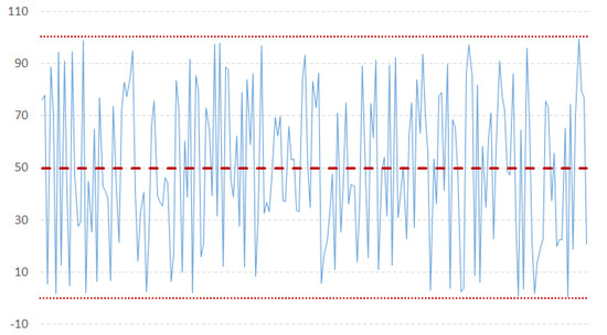 Figure 3. Example of a stationary time series.
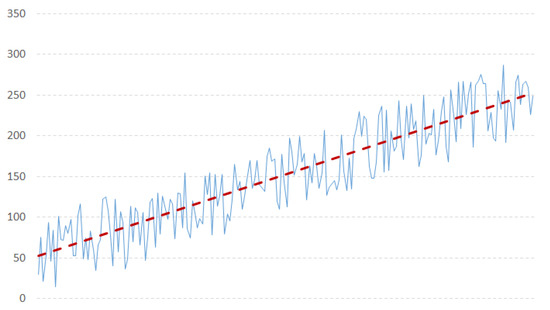 Figure 4. Example of a not stationary time series.
 - Parameters estimation: Within the domain of time series, two important functions deal with lags. The first, the Partial AutoCorrelation Function (PACF), is the correlation between a time series and its own lagged values. The other, the AutoCorrelation Function (ACF), defines how points are correlated with each other, based on how many time steps they are separated by. These two functions are necessary for time series analysis as they are able to identify the extent of the lag in an autoregressive model (PACF) and in a moving average model (ACF) [50].Figure 5 and Figure 6 show an example of an ACF and PACF. The use of these functions was introduced as part of the Box–Jenkins approach to time series modeling, where computing the partial autocorrelation function could be determined by the appropriate lags p in an ARIMA (p, d, q) model, and computing the autocorrelation function could be determined by the appropriate lag q in an ARIMA (p, d, q) model. Because the (partial) autocorrelation of a MA(q) (AR(p)) process is zero at lag q + 1 (p + 1) and higher, we take into account the sample (partial) autocorrelation function to check where it becomes zero (any departure from zero). This is achieved by considering a 95% confidence interval for the sample (partial) autocorrelation plot. The confidence band is approximately , where N corresponds to the sample size.
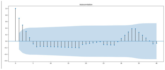 Figure 5. Example of an ACF plot. This plot shows a spike for lag values less than 4, based on 95% confidential criteria. So we choose a q value of 4 for the upper bound when we are searching for best (p, d, q) configuration.
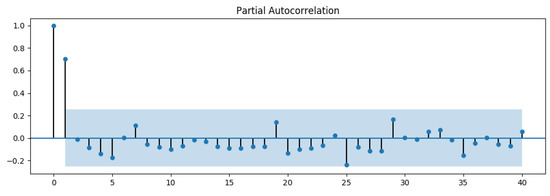 Figure 6. Example of a PACF plot. This plot shows a spike for lag values less than 2, based on 95% confidential criteria. So we choose a p value of 2 for the upper bound when we’re searching for best ( p, d, q) configuration.More informations about p and q estimation and their importance is highlighted by authors in [33].
 - Model evaluation: To determine the best ARIMA model for the Amazon products, we always perform the following steps:
- -
- check stationarity, with the Ng and Perron modified unit root test [31], useful also to find an appropriate d value.
- -
- find p and q based on PACF and ACF. The result on ACF and PACF gives us an upper bound for iterating the fitting of the model, keeping the best combination, based on the least MSE value, described as:where is a vector of n predictions, and Y is the vector of the observed values of the variable being predicted.
5.2.2. Algorithm
This section describes how we applied ARIMA to our study. As mentioned above, we have different features (as time series) that can be used as exogenous variables for our ARIMA model. An exogenous variable would contain tuples in the form of (date, value). For instance, in terms of tuples, when merging the Amazon products’ prices Basic data with Google Trends data we will have to join (date, price) with (date, popularity) so that we will obtain (date, popularity, price) tuples that can be fed to ARIMA. Thus, the algorithm we perform for each product of our collection is:
- perform data retrieving - Retrieve products’ external data. For instance, if a product has Google Trends entries for itsManufacturerwe retrieve that and add it to the current external features.
- Model Fit - Fit a model for each combination of products’ available basic and external features.
Formally we can express the points above as follows: given an item I, we retrieve its available data (features) that can be split in two subsets of features such that:
where P is a function that takes and as inputs and returns a new set of features that contains all the elements of and a possible combination of (also ∅). The function C returns all the possible combinations of features in :
Once we obtain all the features combinations we proceed to fit the ARIMA model with each of the features combinations above coupled with their correlated MAPE and saving these results as a (Map[Fitted Model, MAPE Score]) defined as , . Let be the real trend described by .
Although in some studies, such as that in [51], the MAPE metric has been computed by using the median instead of the mean, during the experiments we preferred to adopt its canonical formulation (i.e., that based on the mean) in order to have the opportunity to compare our results to other works in literature, since it represents the most widely used evaluation metric in forecasting fields [52,53].
is defined as:
Taking a real price trend and a forecast makes the difference for each point with the same date field by accessing them with an index j. It sums all of these differences and returns a percentage error of the average difference between all the points considered. More about MAPE can be read in [54].
To obtain the results, we simply look for the value in m having the lowest value. It means that the key such that is the best combination of features for the underlying product. Thus, different Amazon products might have different combinations of features as best configuration. The code we have developed to implement the proposed ARIMA model can be freely downloaded (github.com/andream16/price-probe-ml).
6. Performance Evaluation
In this section, we will include the experiments we performed, and the results we obtained.
Methodology
For experiment purposes we considered the top 100,000 Amazon products with the highest number of prices entries. We used three different test sizes, 10%, 20% and 30% related to the prices entries of each product. Test size reflects the number of predictions made. Thus, for a given product having a time series of 100 prices elements, if we have a test set size of 10%, we will use the first 90 elements to train the model, and will perform the forecast on the last 10 elements left calculating the related MAPE. We calculated the prediction for the other two test sizes (20% and 30%) similarly. For each percentage, we have used the time series cross-validation function offered by scikit-learn Python library and detailed here (https://towardsdatascience.com/time-series-nested-cross-validation-76adba623eb9) and in compliance with research work performed by authors in [55]. We have used several combinations of features as exogenous variables for products and in Table 1 we indicate how many times a given feature has been found within the 100,000 Amazon products of our analysis.

Table 1.
Occurrences of extracted features within 100,000 collected products and their percentage.
We recall that we used the manufacturer exclusively to extract the Google Trends time series of the products. Therefore the manufacturer has not been used as an exogenous variable for the ARIMA model whereas Google Trends has. Also, the reader might notice how the co-occurrences of multiple features (e.g., (manufacturer, trend) or (manufacturer, sentiment)) is lower than that of single features. In Table 2 we include the MAPE values for each combination of exogenous variables we used for the three different test sets size.
Table 2.
MAPE values for the three different test sets and their average for time series with tuples.
In most of the cases, decreasing values for the test size corresponds to more accurate scores of the prediction. In particular, we can observe that (price, date, Google Trends) combination (that is, Google Trends represents the single exogenous variable) is the most promising setting, having the lowest Average MAPE. We have carried out a statistical test using the Diebold-Mariano test [56] (https://www.real-statistics.com/time-series-analysis/forecasting-accuracy/diebold-mariano-test/) which confirmed that the MAPE results we obtained using Google Trends and Sentiment as exogenous variables are better than those obtained using just Sentiment which is, in turn, better than the MAPEs obtained using Google Trends as exogenous variable.
In support of that, in Table 3 we have highlighted the number of products out of 100,000 having the manufacturer information, how many manufacturers have Google Trends information and how many times the tuple (price, date, Google Trends) has been the best combination among the others for our three test dataset size. The second and third columns are related to the entire collection of 100,000 products and, therefore, they have the same number of the three datasets. The last column indicates how often combination has been the best with respect to the others.
Table 3.
Manufacturer and Google Trends occurrences and percentage indicating how often Google Trends has been the best exogenous variable.
For the test size of 10% Google Trends as exogenous variable has been found the best combination for 61% of the total products. This clearly indicates a strong correlation between Google Trends and the price of Amazon products. By decreasing the size of the test set, ARIMA model is trained with a smaller amount of data and, they are less robust to predict the remainder data with high accuracy. We have also counted how many times the sentiment information brings benefit to the prediction process but the numbers (the combination including sentiment information has been the best combination less than 4% of the times) indicate very low correlation showing a disconnection with Amazon products’ prices.
7. Conclusions and Future Directions
The number of online sales is growing quickly and customers do not have a clear idea of how prices are influenced aside sale times. Having a way to predict such a thing would help customers making better choices regarding which marketplace to use in order to purchase a certain product or in which period. We have shown how Price Probe predicts Amazon prices, one of the biggest E-Shop players, indicating high precision in the forecast through ARIMA, fine-tuning local parameters and especially when using Google Trends as exogenous variable. Our method highly depends on how external features have been chosen and collected. It would be interesting to use more external features (for instance the popularity of a specific product on Twitter or the reviews given in Google products or other website) about the product’s popularity over time, since we highlighted only how Google Trends influences our results. The future of purchases relies on online marketplaces and Price Probe might be used to predict when it might be more profitable to purchase a certain product. In addition, it should be observed that our experiments involved a very large amount of data, with regard to similar works in literature based on similar data dimensions [17,44].
As next steps, we aim at employing neural networks for a similar evaluation presented in this paper although we will need to find a way to include information from Google Trends within the layers of the network. Moreover, we would like to focus on problems within the financial technology domain. In particular, one of the goals we aim to tackle is to analyse stock markets and their trends and perform forecast of long and short operations by including information coming from social networks (e.g., Facebook, Twitter, StockTwits, etc.), news and any other kind of data that can be extracted and associated with the stock markets values that we already have (we are already using a platform known as MultiCharts where we can extract all the time series of each stock market for every interval time and for each granularity—starting from 5 minutes range). Moreover, one more direction is related to the computational complexity: we would like to follow the work suggested in [45] for parameters estimation in order to keep low the complexity of the problem.
Author Contributions
S.C. provided analysis and suggestions for the analysis of data. A.M. and A.P. worked on the extraction of the data. R.S. tuned the ARIMA model and D.R.R. carried out the performance evaluation and drafted the first version of the paper.
Funding
This research was funded by Regione Sardegna, CUP F74G14000200008 F19G14000910008.
Acknowledgments
This research is partially funded by: Regione Sardegna under project Next generation Open Mobile Apps Development (NOMAD), Pacchetti Integrati di Agevolazione (PIA)—Industria Artigianato e Servizi—Annualità 2013; Italian Ministry of Education, University and Research—Program Smart Cities and Communities and Social Innovation project ILEARNTV (D.D. n.1937 del 05.06.2014, CUP F74G14000200008 F19G14000910008).
Conflicts of Interest
The authors declare no conflict of interest.
References
- Zimmermann, S.; Herrmann, P.; Kundisch, D.; Nault, B. Decomposing the Variance of Consumer Ratings and the Impact on Price and Demand. Inf. Syst. Res. 2018. [Google Scholar] [CrossRef]
- Cavalcante, R.C.; Brasileiro, R.C.; Souza, V.L.; Nobrega, J.P.; Oliveira, A.L. Computational Intelligence and Financial Markets: A Survey and Future Directions. Expert Syst. Appl. 2016, 55, 194–211. [Google Scholar] [CrossRef]
- Atsalakis, G.S.; Valavanis, K.P. Surveying stock market forecasting techniques—Part II: Soft computing methods. Expert Syst. Appl. 2009, 36, 5932–5941. [Google Scholar] [CrossRef]
- Pai, P.F.; Lin, C.S. A hybrid ARIMA and support vector machines model in stock price forecasting. Omega 2005, 33, 497–505. [Google Scholar] [CrossRef]
- Conejo, A.J.; Plazas, M.A.; Espinola, R.; Molina, A.B. Day-ahead electricity price forecasting using the wavelet transform and ARIMA models. IEEE Trans. Power Syst. 2005, 20, 1035–1042. [Google Scholar] [CrossRef]
- Jadhav, V.; Chinnappa Reddy, B.; Gaddi, G. Application of ARIMA model for forecasting agricultural prices. J. Agric. Sci. Technol. 2017, 19, 981–992. [Google Scholar]
- Wang, Y.; Wang, C.; Shi, C.; Xiao, B. Short-term cloud coverage prediction using the ARIMA time series model. Remote Sens. Lett. 2018, 9, 274–283. [Google Scholar] [CrossRef]
- Rangel-González, J.A.; Frausto-Solis, J.; Javier González-Barbosa, J.; Pazos-Rangel, R.A.; Fraire-Huacuja, H.J. Comparative Study of ARIMA Methods for Forecasting Time Series of the Mexican Stock Exchange. In Fuzzy Logic Augmentation of Neural and Optimization Algorithms: Theoretical Aspects and Real Applications; Castillo, O., Melin, P., Kacprzyk, J., Eds.; Springer: Cham, Germany, 2018; pp. 475–485. [Google Scholar] [CrossRef]
- Jiang, S.; Yang, C.; Guo, J.; Ding, Z. ARIMA forecasting of China’s coal consumption, price and investment by 2030. Energy Sources Part B Econ. Plan. Policy 2018, 13, 190–195. [Google Scholar] [CrossRef]
- Ozturk, S.; Ozturk, F. Forecasting Energy Consumption of Turkey by Arima Model. J. Asian Sci. Res. 2018, 8, 52–60. [Google Scholar] [CrossRef]
- Bennett, C.; Stewart, R.A.; Lu, J. Autoregressive with exogenous variables and neural network short-term load forecast models for residential low voltage distribution networks. Energies 2014, 7, 2938–2960. [Google Scholar] [CrossRef]
- Bakir, H.; Chniti, G.; Zaher, H. E-Commerce Price Forecasting Using LSTM Neural Networks. Int. J. Mach. Learn. Comput. 2018, 8, 169–174. [Google Scholar] [CrossRef]
- Liu, W.W.; Liu, Y.; Chan, N.H. Modeling eBay Price Using Stochastic Differential Equations. J. Forecast. 2018. [Google Scholar] [CrossRef]
- Hand, C.; Judge, G. Searching for the picture: forecasting UK cinema admissions using Google Trends data. Appl. Econ. Lett. 2012, 19, 1051–1055. [Google Scholar] [CrossRef]
- Bangwayo-Skeete, P.F.; Skeete, R.W. Can Google data improve the forecasting performance of tourist arrivals? Mixed-data sampling approach. Tour. Manag. 2015, 46, 454–464. [Google Scholar] [CrossRef]
- Wei, W.W.S. Time Series Analysis: Univariate and Multivariate Methods; Pearson Addison Wesley: Boston, MA, USA, 2006. [Google Scholar]
- Tyralis, H.; Papacharalampous, G. Variable selection in time series forecasting using random forests. Algorithms 2017, 10, 114. [Google Scholar] [CrossRef]
- Papacharalampous, G.; Tyralis, H.; Koutsoyiannis, D. One-step ahead forecasting of geophysical processes within a purely statistical framework. Geosci. Lett. 2018, 5, 12. [Google Scholar] [CrossRef]
- Meyler, A.; Kenny, G.; Quinn, T. Forecasting Irish Inflation Using ARIMA Models; Central Bank of Ireland: Dublin, Ireland, 1998. [Google Scholar]
- Geetha, A.; Nasira, G. Time-series modelling and forecasting: Modelling of rainfall prediction using ARIMA model. Int. J. Soc. Syst. Sci. 2016, 8, 361–372. [Google Scholar] [CrossRef]
- Pincheira, P.; Hardy, N. Forecasting Base Metal Prices with Commodity Currencies; MPRA Paper 83564; University Library of Munich: Munich, Germany, 2018. [Google Scholar]
- Hong, T.; Fan, S. Probabilistic electric load forecasting: A tutorial review. Int. J. Forecast. 2016, 32, 914–938. [Google Scholar] [CrossRef]
- Yu, L.; Zhao, Y.; Tang, L.; Yang, Z. Online big data-driven oil consumption forecasting with Google trends. Int. J. Forecast. 2018. [Google Scholar] [CrossRef]
- Szczech, M.; Turetken, O. The Competitive Landscape of Mobile Communications Industry in Canada: Predictive Analytic Modeling with Google Trends and Twitter. In Analytics and Data Science: Advances in Research and Pedagogy; Deokar, A.V., Gupta, A., Iyer, L.S., Jones, M.C., Eds.; Springer: Cham, Germany, 2018; pp. 143–162. [Google Scholar] [CrossRef]
- Tuladhar, J.G.; Gupta, A.; Shrestha, S.; Bania, U.M.; Bhargavi, K. Predictive Analysis of E-Commerce Products. In Intelligent Computing and Information and Communication; Bhalla, S., Bhateja, V., Chandavale, A.A., Hiwale, A.S., Satapathy, S.C., Eds.; Springer: Singapore, 2018; pp. 279–289. [Google Scholar]
- Tseng, K.K.; Lin, R.F.Y.; Zhou, H.; Kurniajaya, K.J.; Li, Q. Price prediction of e-commerce products through Internet sentiment analysis. Electron. Commer. Res. 2018, 18, 65–88. [Google Scholar] [CrossRef]
- Guo, K.; Sun, Y.; Qian, X. Can investor sentiment be used to predict the stock price? Dynamic analysis based on China stock market. Phys. A Stat. Mech. Appl. 2017, 469, 390–396. [Google Scholar] [CrossRef]
- Brockwell, P.J.; Davis, R.A. Introduction. In Introduction to Time Series and Forecasting; Springer: Cham, Germany, 2016; pp. 1–37. [Google Scholar] [CrossRef]
- Dickey, D.A.; Fuller, W.A. Distribution of the Estimators for Autoregressive Time Series with a Unit Root. J. Am. Stat. Assoc. 1979, 74, 427–431. [Google Scholar]
- Dickey, D.A.; Fuller, W.A. Likelihood Ratio Statistics for Autoregressive Time Series with a Unit Root. Econometrica 1981, 49, 1057–1072. [Google Scholar] [CrossRef]
- Ng, S.; Perron, P. Lag Length Selection and the Construction of Unit Root Tests with Good Size and Power. Econometrica 2001, 69, 1519–1554. [Google Scholar] [CrossRef]
- Box, G.E.P.; Jenkins, G. Time Series Analysis, Forecasting and Control; Holden-Day, Incorporated: San Francisco, CA, USA, 1990. [Google Scholar]
- Ke, Z.; Zhang, Z.J. Testing autocorrelation and partial autocorrelation: Asymptotic methods versus resampling techniques. Br. J. Math. Stat. Psychol. 2018, 71, 96–116. [Google Scholar] [CrossRef] [PubMed]
- Seabold, S.; Perktold, J. Statsmodels: Econometric and statistical modeling with python. In Proceedings of the 9th Python in Science Conference, Austin, TX, USA, 28 June–3 July 2010. [Google Scholar]
- Valipour, M.; Banihabib, M.E.; Behbahani, S.M.R. Comparison of the ARMA, ARIMA, and the autoregressive artificial neural network models in forecasting the monthly inflow of Dez dam reservoir. J. Hydrol. 2013, 476, 433–441. [Google Scholar] [CrossRef]
- Zhang, G.; Xu, L.; Xue, Y. Model and forecast stock market behavior integrating investor sentiment analysis and transaction data. Clust. Comput. 2017, 20, 789–803. [Google Scholar] [CrossRef]
- Ho-Dac, N.N.; Carson, S.J.; Moore, W.L. The effects of positive and negative online customer reviews: Do brand strength and category maturity matter? J. Mark. 2013, 77, 37–53. [Google Scholar] [CrossRef]
- Goh, K.Y.; Heng, C.S.; Lin, Z. Social media brand community and consumer behavior: Quantifying the relative impact of user-and marketer-generated content. Inf. Syst. Res. 2013, 24, 88–107. [Google Scholar] [CrossRef]
- Goes, P.B.; Lin, M.; Au Yeung, C.M. “Popularity effect” in user-generated content: Evidence from online product reviews. Inf. Syst. Res. 2014, 25, 222–238. [Google Scholar] [CrossRef]
- Kim, Y.; Srivastava, J. Impact of social influence in e-commerce decision making. In Proceedings of the Ninth International Conference on Electronic Commerce, Minneapolis, MN, USA, 19–22 August 2007; pp. 293–302. [Google Scholar]
- Gilbert, C.H.E. Vader: A parsimonious rule-based model for sentiment analysis of social media text. In Proceedings of the Eighth International Conference on Weblogs and Social Media (ICWSM-14), Ann Arbor, MI, USA, 1–4 June 2014; Available online: http://comp. social. gatech.edu/papers/icwsm14.vader.hutto.pdf (accessed on 21 December 2018).
- Velicer, W.F.; Colby, S.M. A Comparison of Missing-Data Procedures for Arima Time-Series Analysis. Educ. Psychol. Meas. 2005, 65, 596–615. [Google Scholar] [CrossRef]
- Hyndman, R.J.; Athanasopoulos, G. Forecasting: Principles and Practice; OTexts: Melbourne, Australia, 2018. [Google Scholar]
- Papacharalampous, G.; Tyralis, H.; Koutsoyiannis, D. Predictability of monthly temperature and precipitation using automatic time series forecasting methods. Acta Geophys. 2018, 66, 807–831. [Google Scholar] [CrossRef]
- Hyndman, R.J.; Khandakar, Y. Automatic Time Series Forecasting: The forecast Package for R. J. Stat. Softw. 2008, 27. [Google Scholar] [CrossRef]
- Box, G.E.; Jenkins, G.M. Some recent advances in forecasting and control. J. R. Stat. Soc. Ser. C (Appl. Stat.) 1968, 17, 91–109. [Google Scholar] [CrossRef]
- Taieb, S.B.; Bontempi, G.; Atiya, A.F.; Sorjamaa, A. A review and comparison of strategies for multi-step ahead time series forecasting based on the NN5 forecasting competition. Expert Syst. Appl. 2012, 39, 7067–7083. [Google Scholar] [CrossRef]
- Khobai, H.; Chitauro, M. The Impact of Trade Liberalisation on Economic Growth in Switzerland. 2018. Available online: https://mpra.ub.uni-muenchen.de/89884/ (accessed on 21 December 2018).
- Lopes, S.R.C.; Olbermann, B.P.; Reisen, V.A. Non-stationary Gaussian ARFIMA processes: Estimation and application. Braz. Rev. Econom. 2002, 22, 103–126. [Google Scholar] [CrossRef]
- Flores, J.H.F.; Engel, P.M.; Pinto, R.C. Autocorrelation and partial autocorrelation functions to improve neural networks models on univariate time series forecasting. In Proceedings of the 2012 International Joint Conference on Neural Networks (IJCNN), Brisbane, Australia, 10–15 June 2012; pp. 1–8. [Google Scholar] [CrossRef]
- Armstrong, J.S.; Collopy, F. Error measures for generalizing about forecasting methods: Empirical comparisons. Int. J. Forecast. 1992, 8, 69–80. [Google Scholar] [CrossRef]
- Yang, W.; Wang, J.; Niu, T.; Du, P. A hybrid forecasting system based on a dual decomposition strategy and multi-objective optimization for electricity price forecasting. Appl. Energy 2019, 235, 1205–1225. [Google Scholar] [CrossRef]
- Mehmanpazir, F.; Asadi, S. Development of an evolutionary fuzzy expert system for estimating future behavior of stock price. J. Ind. Eng. Int. 2017, 13, 29–46. [Google Scholar] [CrossRef]
- de Myttenaere, A.; Golden, B.; Grand, B.L.; Rossi, F. Mean Absolute Percentage Error for regression models. Neurocomputing 2016, 192, 38–48. [Google Scholar] [CrossRef]
- Afendras, G.; Markatou, M. Optimality of training/test size and resampling effectiveness in cross-validation. J. Stat. Plan. Inference 2019, 199, 286–301. [Google Scholar] [CrossRef]
- Diebold, F.X. Comparing Predictive Accuracy, Twenty Years Later: A Personal Perspective on the Use and Abuse of Diebold–Mariano Tests. J. Bus. Econ. Stat. 2015, 33, 1. [Google Scholar] [CrossRef]
© 2018 by the authors. Licensee MDPI, Basel, Switzerland. This article is an open access article distributed under the terms and conditions of the Creative Commons Attribution (CC BY) license (http://creativecommons.org/licenses/by/4.0/).