
Thermodynamic Balance vs. Computational Fluid Dynamics Approach for the Outlet Temperature Estimation of a Benchtop Spray Dryer

 , , , , and
Abstract
:
1. Introduction
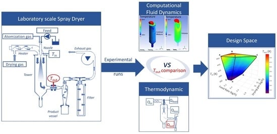
2. Materials and Methods
2.1. Experiments and Measurements
2.2. Experimental Design
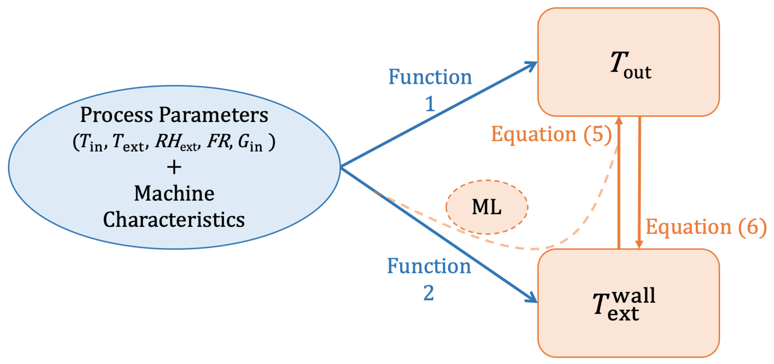
2.3. Thermodynamic Model Development
- air is treated as an ideal gas;
- steady-state conditions;
- the inner surface of the spray dryer is smooth;
- the thermal conductivity values of the air () at is linear in the range of the experimental temperatures [24];
- the heat transfer coefficient of inside convection can be calculated using the average temperature .
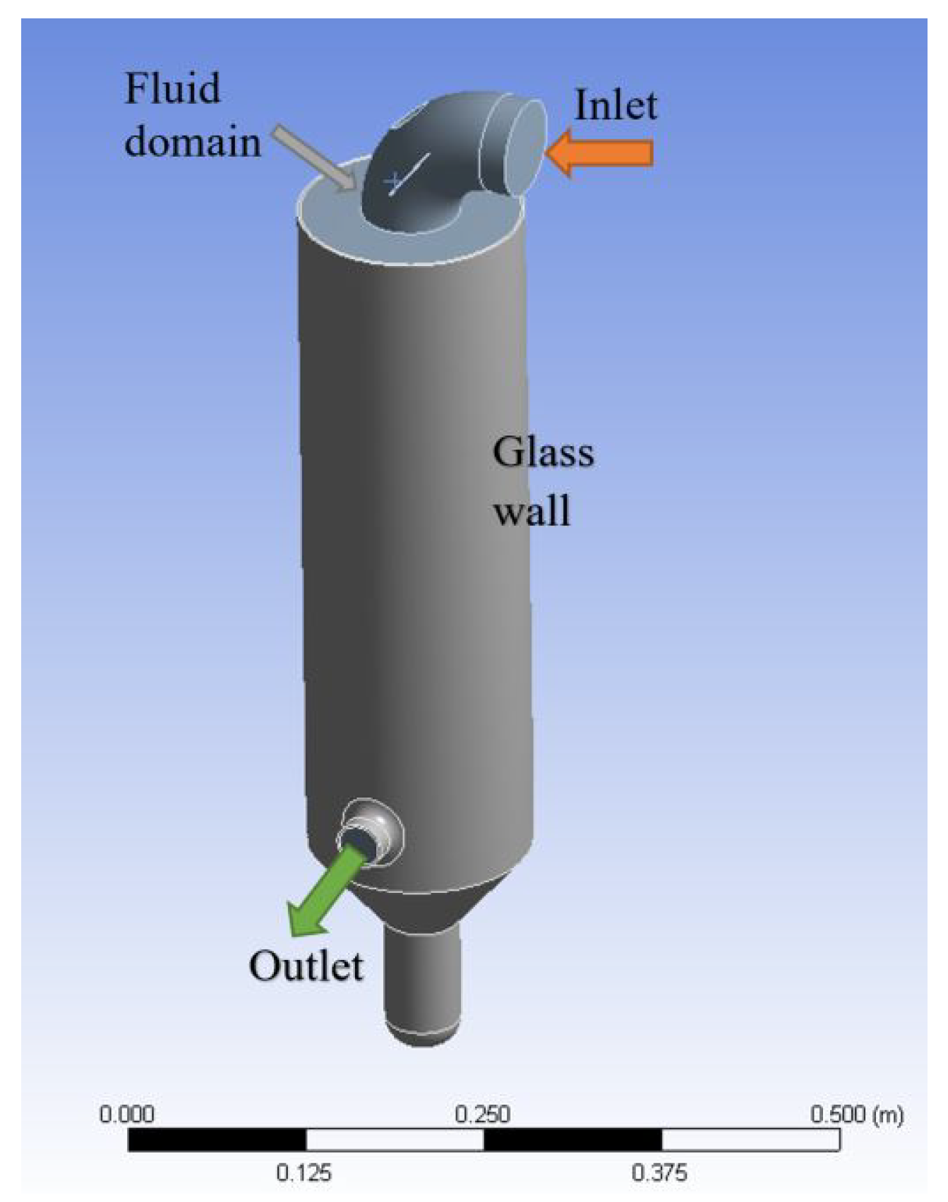
2.4. CFD
- at the inlet: the hot air velocity and temperature;
- at the nozzle: the uniform mixture (water and cold air) velocity, the temperature, and the volume fraction of the water;
- at the outlet: the ambient pressure.
2.5. Models Comparison
3. Results and Discussion
3.1. Experimental Results
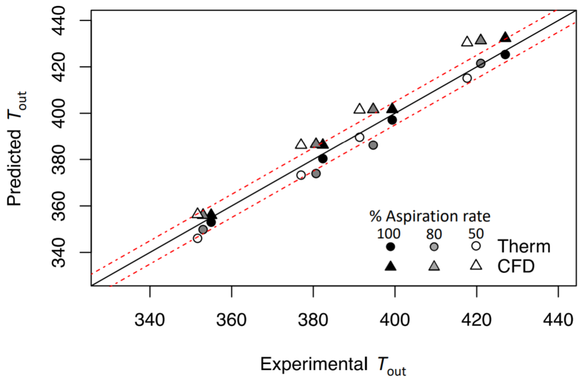
3.2. Thermodynamic Model
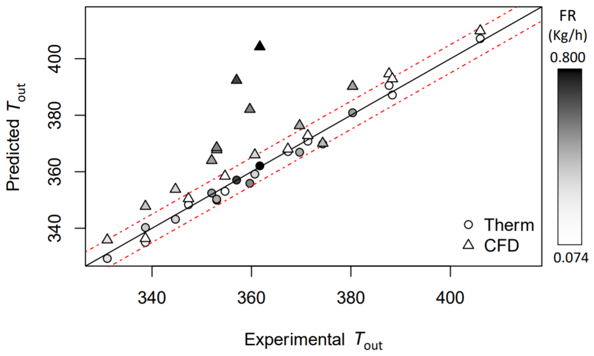
3.3. CFD
3.4. Models Comparison
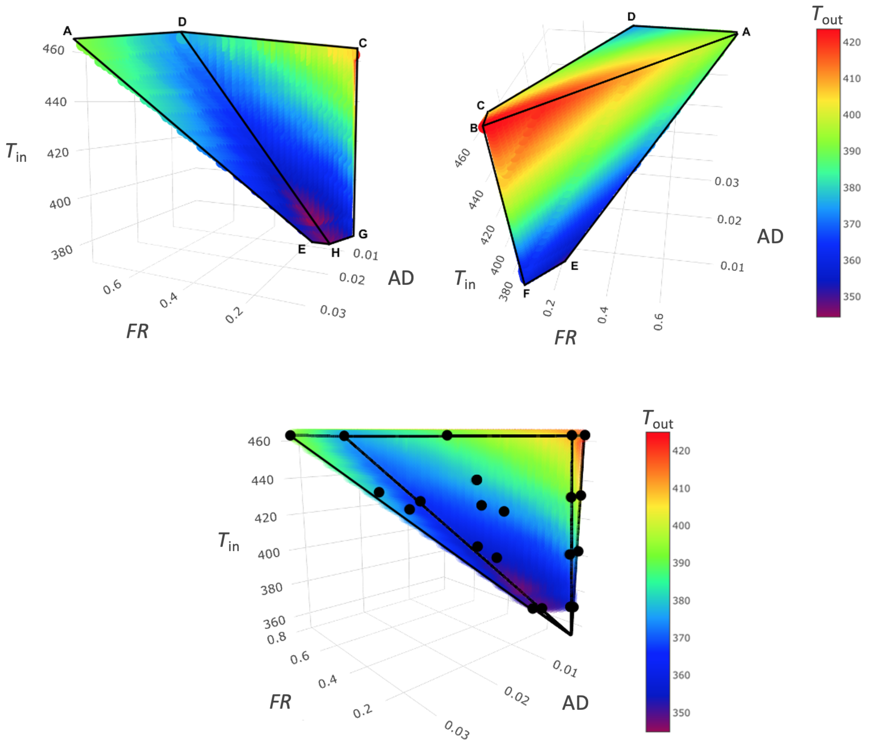
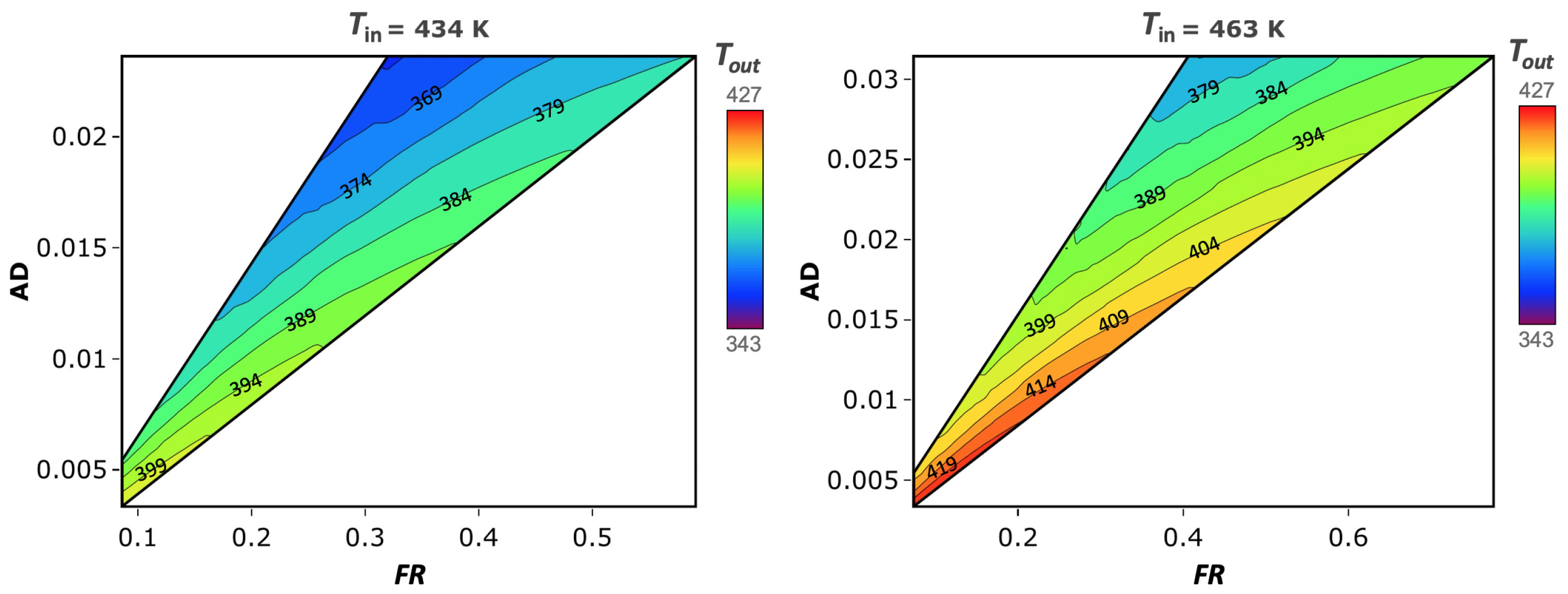
3.5. Spray Drying Design Space
4. Conclusions
Supplementary Materials
Author Contributions
Funding
Institutional Review Board Statement
Informed Consent Statement
Data Availability Statement
Conflicts of Interest
Abbreviations
| CFD | Computational fluid dynamics |
| ML | Machine learning |
| Inlet temperature of the drying gas (K) | |
| Outlet temperature of the drying gas (K) | |
| Environmental temperature (K) | |
| Average temperature of inlet and outlet (K) | |
| Temperature of the spray dryer’s outer surface (K) | |
| Glass-transition temperature (K) | |
| Environmental relative humidity | |
| Drying gas flow rate (kg/h) | |
| Drying gas speed (m/s) | |
| Feed flow rate (kg/h) | |
| Concentration of the feed | |
| Heat entering spray drying (kJ/h) | |
| Heat coming out of the equipment (kJ/h) | |
| Heat required to dry the feed (kJ/h) | |
| Heat lost to the external environment (kJ/h) | |
| Heat lost by convection and conduction (kJ/h) | |
| Heat lost by radiation (kJ/h) | |
| Thermal conductivity of the air (kJ/kg·K) | |
| Heat emissivity coefficient of the glass | |
| External surface of the semplified spray dryer (m) |
References
- Santos, D.; Maurício, A.C.; Sencadas, V.; Santos, J.D.; Fernandes, M.H.; Gomes, P.S. Spray drying: An overview. In Biomaterials; IntechOpen: Rijeka, Croatia, 2018; Volume 2, pp. 11–31. [Google Scholar]
- Bari, E.; Arciola, C.R.; Vigani, B.; Crivelli, B.; Moro, P.; Marrubini, G.; Sorrenti, M.; Catenacci, L.; Bruni, G.; Chlapanidas, T.; et al. In Vitro Effectiveness of Microspheres Based on Silk Sericin and Chlorella vulgaris or Arthrospira platensis for Wound Healing Applications. Materials 2017, 10, 983. [Google Scholar] [CrossRef] [PubMed] [Green Version]
- Emami, F.; Vatanara, V.; Park, E.J.; Na, D.H. Drying technologies for the stability and bioavailability of biopharmaceuticals. Pharmaceutics 2018, 10, 131. [Google Scholar] [CrossRef] [Green Version]
- Bari, E.; Perteghella, S.; Marrubini, G.; Sorrenti, M.; Catenacci, L.; Tripodo, G.; Mastrogiacomo, M.; Mandracchia, D.; Trapani, A.; Faragò, S.; et al. In vitro efficacy of silk sericin microparticles and platelet lysate for intervertebral disk regeneration. Int. J. Biol. Macromol. 2018, 118, 792–799. [Google Scholar] [CrossRef]
- Giovannelli, L.; Milanesi, A.; Ugazio, E.; Fracchia, L.; Segale, L. Effect of Methyl-β-Cyclodextrin and Trehalose on the Freeze–Drying and Spray–Drying of Sericin for Cosmetic Purposes. Pharmaceuticals 2021, 14, 262. [Google Scholar] [CrossRef]
- Pinto, J.T.; Faulhammer, E.; Dieplinger, J.; Dekner, M.; Makert, C.; Nieder, M.; Paudel, A. Progress in spray-drying of protein pharmaceuticals: Literature analysis of trends in formulation and process attributes. Dry. Technol. 2021, 39, 1415–1446. [Google Scholar] [CrossRef]
- Poozesh, S.; Bilgili, E. Scale-up of pharmaceutical spray drying using scale-up rules: A review. Int. J. Pharm. 2019, 562, 271–292. [Google Scholar] [CrossRef] [PubMed]
- Anandharamakrishnan, C.; Padma Ishwarya, S. Spray Drying Techniques for Food Ingredient Encapsulation; John Wiley & Sons, Ltd.: Hoboken, NJ, USA, 2015; Chapter 1; pp. 1–36. [Google Scholar]
- Písecký, J. Handbook of Milk Powder Manufacture, 2nd ed.; GEA Process Engineering A/S: Copenhagen, Denmark, 2012. [Google Scholar]
- Boel, E.; Koekoekx, R.; Dedroog, S.; Babkin, I.; Vetrano, M.R.; Clasen, C.; Van den Mooter, G. Unraveling particle formation: From single droplet drying to spray drying and electrospraying. Pharmaceutics 2020, 12, 625. [Google Scholar] [CrossRef]
- Littringer, E.M.; Paus, R.; Mescher, A.; Schroettner, H.; Walzel, P.; Urbanetz, N.A. The morphology of spray dried mannitol particles—The vital importance of droplet size. Powder Technol. 2013, 239, 162–174. [Google Scholar] [CrossRef]
- Anandharamakrishnan, C.; Rielly, C.D.; Stapley, A.G.F. Effects of process variables on the denaturation of whey proteins during spray drying. Dry. Technol. 2007, 25, 799–807. [Google Scholar] [CrossRef]
- Ziaee, A.; Albadarin, A.B.; Padrela, L.; Ung, M.; Femmer, T.; Walker, G.; O’Reilly, E. A rational approach towards spray drying of biopharmaceuticals: The case of lysozyme. Powder Technol. 2020, 366, 206–215. [Google Scholar] [CrossRef]
- Adhikari, B.; Howes, T.; Lecomte, D.; Bhandari, B.R. A glass transition temperature approch for the prediction of the surface stickiness of a drying droplet during spray drying. Powder Technol. 2005, 149, 168–179. [Google Scholar] [CrossRef] [Green Version]
- Shoji, Y.; McCray, S.; Zhu, C. Stabilization of hac1 influenza vaccine by spray drying: Formulation development and process scale-up. Pharm. Res. 2014, 31, 3006–3018. [Google Scholar]
- Patel, B.B.; Patel, J.K.; Chakraborty, S.; Shukla, D. Revealing facts behind spray dried solid dispersion technology used for solubility enhancement. Saudi Pharm. J. 2015, 23, 352–365. [Google Scholar] [CrossRef] [PubMed] [Green Version]
- Peterson, J.J. A bayesian approach to the ich q8 definition of design space. J. Biopharm. Stat. 2008, 18, 959–975. [Google Scholar] [CrossRef]
- Lebrun, P.; Krier, F.; Mantanus, J.; Grohganz, H.; Yang, M.; Rozet, E.; Boulanger, B.; Evrard, B.; Rantanen, J.; Hubert, P. Design space approach in the optimization of the spray-drying process. Eur. J. Pharm. Biopharm. 2012, 80, 226–234. [Google Scholar] [CrossRef]
- Dohrn, S.; Rawal, P.; Luebbert, C.; Lehmkemper, K.; Kyeremateng, S.O.; Degenhardt, M.; Sadowski, G. Predicting process design spaces for spray drying amorphous solid dispersions. Int. J. Pharm. X 2021, 3, 100072. [Google Scholar] [CrossRef]
- Dobry, D.E.; Settell, D.M.; Baumann, J.M.; Ray, R.J.; Graham, L.J.; Beyerinck, R.A. A model-based methodology for spray-drying process development. J. Pharm. Innov. 2009, 4, 133–142. [Google Scholar] [CrossRef] [Green Version]
- Lisboa, H.M.; Duarte, M.E.; Cavalcanti-Mata, M.E. Modeling of food drying processes in industrial spray dryers. Food Bioprod. Process. 2018, 107, 49–60. [Google Scholar] [CrossRef]
- da Silva, C.R.; Martins, E.; Silveira, A.C.P.; Simeão, M.; Mendes, A.L.; Perrone, Í.T.; Schuck, P.; de Carvalho, A.F. Thermodynamic characterization of single-stage spray dryers: Mass and energy balances for milk drying. Dry. Technol. 2017, 35, 1791–1798. [Google Scholar] [CrossRef]
- Grasmeijer, N.; de Waard, H.; Hinrichs, W.L.J.; Frijlink, H.W. A user-friendly model for spray drying to aid pharmaceutical product development. PLoS ONE 2013, 8, e74403. [Google Scholar] [CrossRef] [Green Version]
- Zografos, A.J.; Martin, W.A.; Sunderland, J.E. Equations of properties as a function of temperature for seven fluids. Comput. Methods Appl. Mech. Eng. 1987, 61, 177–187. [Google Scholar] [CrossRef]
- Lee, W.H. Computational Methods for Two-Phase Flow and Particle Transport; World Scientific: Singapore, 2013. [Google Scholar]
- Cher Pin, S.; Rashmi, W.; Khalid, M.; Chong, C.H.; Woo, M.W.; Tee, L.H. Simulation of spray drying on piper betle linn extracts using computational fluid dynamics. Int. Food Res. J. 2014, 21, 1089–1096. [Google Scholar]
- Maury, M.; Murphy, K.; Kumar, S.; Mauerer, A.; Lee, G. Spray-drying of proteins: Effects of sorbitol and trehalose on aggregation and ft-ir amide i spectrum of an immunoglobulin g. Eur. J. Pharm. Biopharm. 2005, 59, 251–261. [Google Scholar] [CrossRef] [PubMed]
- Çengel, Y.A. Introduction to Thermodynamics and Heat Transfer; McGraw-Hill Education: New York City, NY, USA, 2009. [Google Scholar]


| (K) | % Asp | % | (K) | (kg/h) | (K) |
|---|---|---|---|---|---|
| 100 | 25.6 | 294.0 | 23.8 | 427.0 | |
| 473 | 80 | 34.4 | 299.1 | 20.4 | 421.0 |
| 50 | 24.7 | 295.7 | 13.7 | 417.7 | |
| 100 | 29.5 | 293.7 | 27.8 | 399.3 | |
| 433 | 80 | 22.3 | 297.5 | 22.5 | 394.7 |
| 50 | 26.1 | 293.0 | 16.3 | 391.3 | |
| 100 | 43.7 | 297.4 | 28.4 | 382.3 | |
| 413 | 80 | 35.7 | 298.0 | 24.5 | 380.7 |
| 50 | 35.5 | 298.0 | 16.1 | 377.0 | |
| 100 | 32.6 | 294.2 | 33.8 | 355.0 | |
| 373 | 80 | 24.8 | 298.5 | 26.9 | 353.0 |
| 50 | 32.6 | 294.4 | 19.5 | 351.7 |
| (K) | (K) | (K) | % (K) | FR (kg/h) | (kg/h) | AD |
|---|---|---|---|---|---|---|
| 463 | 296 | 362 | 35.8 | 0.80 | 18.2 | |
| 295 | 360 | 22.9 | 0.42 | 9.4 | ||
| 297 | 406 | 24.0 | 0.07 | 17.5 | ||
| 297 | 388 | 24.0 | 0.07 | 9.3 | ||
| 433 | 297 | 357 | 40.9 | 0.59 | 18.2 | |
| 295 | 353 | 30.3 | 0.32 | 9.4 | ||
| 298 | 388 | 23.7 | 0.07 | 18.7 | ||
| 298 | 371 | 22.8 | 0.07 | 9.8 | ||
| 403 | 294 | 352 | 44.9 | 0.34 | 18.7 | |
| 297 | 345 | 35.6 | 0.21 | 9.8 | ||
| 297 | 367 | 23.8 | 0.07 | 18.7 | ||
| 297 | 355 | 23.8 | 0.07 | 9.8 | ||
| 373 | 295 | 339 | 41.7 | 0.23 | 19.2 | |
| 295 | 331 | 29.1 | 0.17 | 10.3 | ||
| 297 | 347 | 24.2 | 0.07 | 19.3 | ||
| 297 | 339 | 24.2 | 0.07 | 10.1 |
| RMSE (K) | MAE (K) | ||
|---|---|---|---|
| Empty Therm. model | 4.04 | 0.99 | 3.34 |
| Empty CFD model | 7.21 | 0.99 | 6.32 |
| Atom. Therm. model | 2.15 | 0.99 | 1.74 |
| Atom. CFD model | 14.91 | 0.69 | 10.43 |
Publisher’s Note: MDPI stays neutral with regard to jurisdictional claims in published maps and institutional affiliations. |
© 2022 by the authors. Licensee MDPI, Basel, Switzerland. This article is an open access article distributed under the terms and conditions of the Creative Commons Attribution (CC BY) license (https://creativecommons.org/licenses/by/4.0/).
Share and Cite
Milanesi, A.; Rizzuto, F.; Rinaldi, M.; Foglio Bonda, A.; Segale, L.; Giovannelli, L. Thermodynamic Balance vs. Computational Fluid Dynamics Approach for the Outlet Temperature Estimation of a Benchtop Spray Dryer. Pharmaceutics 2022, 14, 296. https://doi.org/10.3390/pharmaceutics14020296
Milanesi A, Rizzuto F, Rinaldi M, Foglio Bonda A, Segale L, Giovannelli L. Thermodynamic Balance vs. Computational Fluid Dynamics Approach for the Outlet Temperature Estimation of a Benchtop Spray Dryer. Pharmaceutics. 2022; 14(2):296. https://doi.org/10.3390/pharmaceutics14020296
Chicago/Turabian StyleMilanesi, Andrea, Francesco Rizzuto, Maurizio Rinaldi, Andrea Foglio Bonda, Lorena Segale, and Lorella Giovannelli. 2022. "Thermodynamic Balance vs. Computational Fluid Dynamics Approach for the Outlet Temperature Estimation of a Benchtop Spray Dryer" Pharmaceutics 14, no. 2: 296. https://doi.org/10.3390/pharmaceutics14020296
APA StyleMilanesi, A., Rizzuto, F., Rinaldi, M., Foglio Bonda, A., Segale, L., & Giovannelli, L. (2022). Thermodynamic Balance vs. Computational Fluid Dynamics Approach for the Outlet Temperature Estimation of a Benchtop Spray Dryer. Pharmaceutics, 14(2), 296. https://doi.org/10.3390/pharmaceutics14020296