Assessing the Spatial and Spatio-Temporal Distribution of Forest Species via Bayesian Hierarchical Modeling


Abstract
:1. Introduction
2. Materials and Methods
2.1. Abies alba Mill.
2.2. Castanea sativa Mill.
2.3. Pinus pinaster Ait.
2.4. Quercus robur L.
2.5. Environmental Variables
2.6. Spatial Model
2.7. Spatio-Temporal Model
2.8. Implementation
3. Results
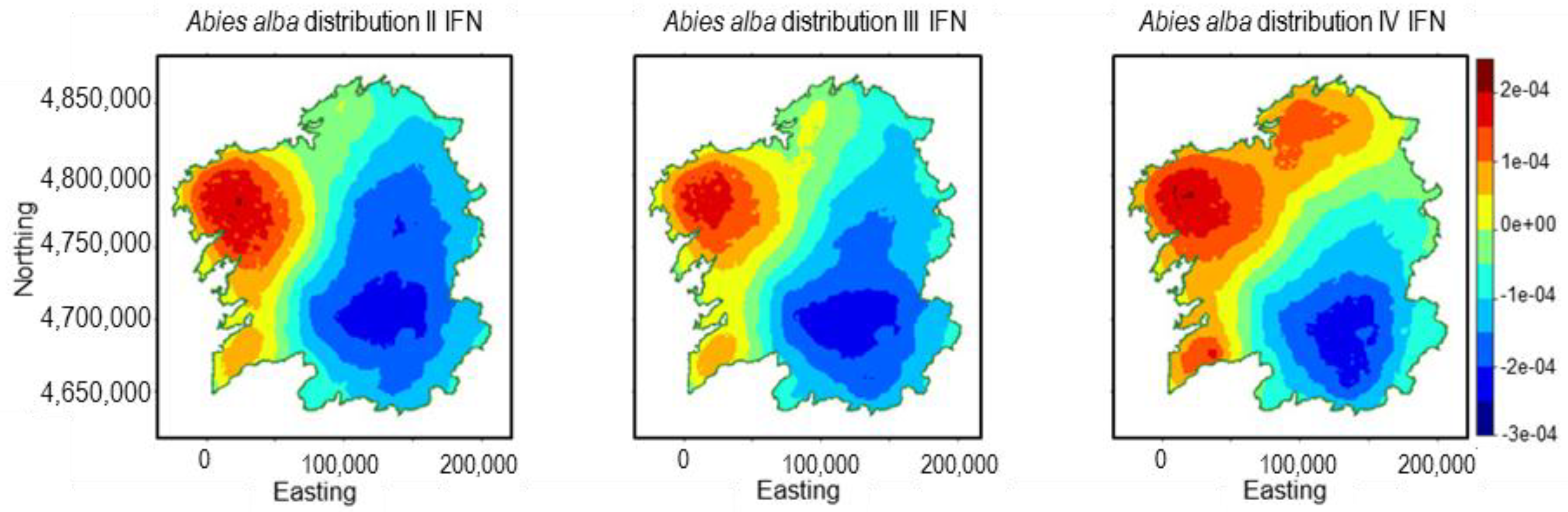
3.1. Abies alba
3.2. Castanea sativa
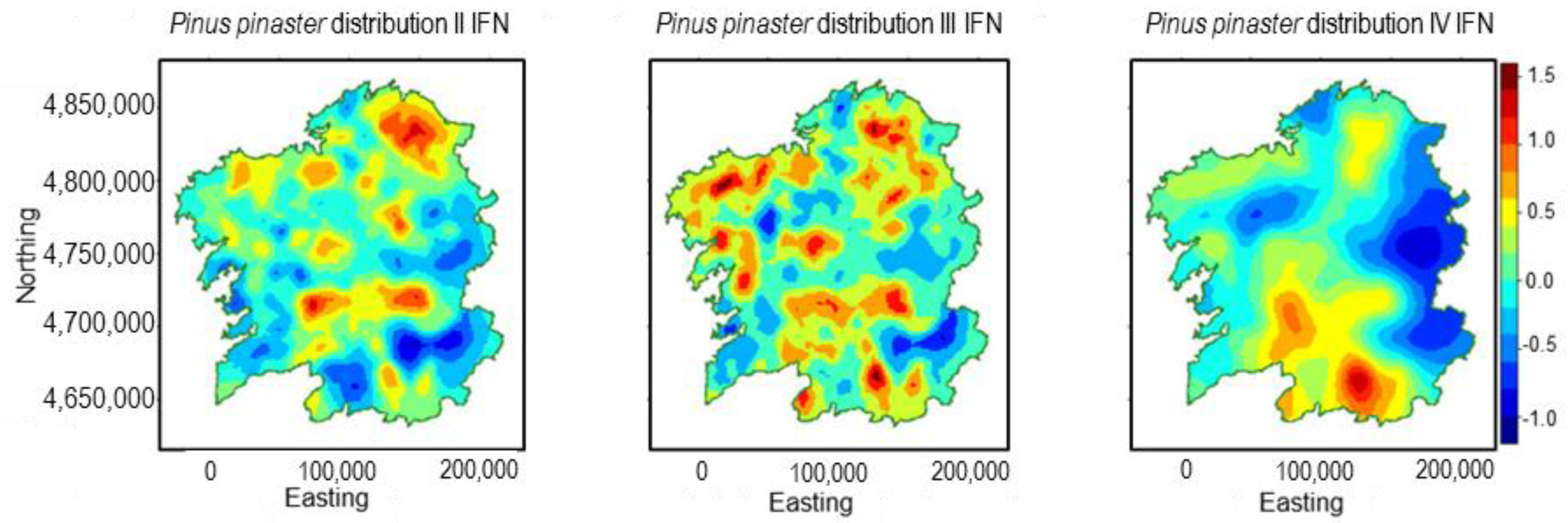
3.3. Pinus pinaster
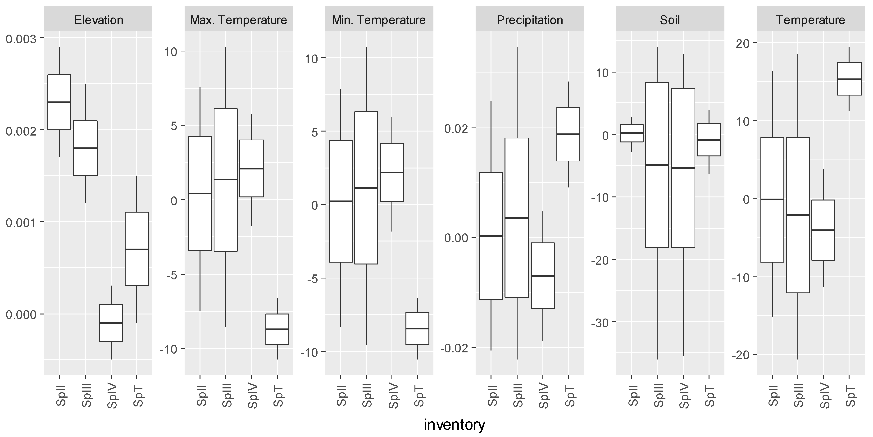
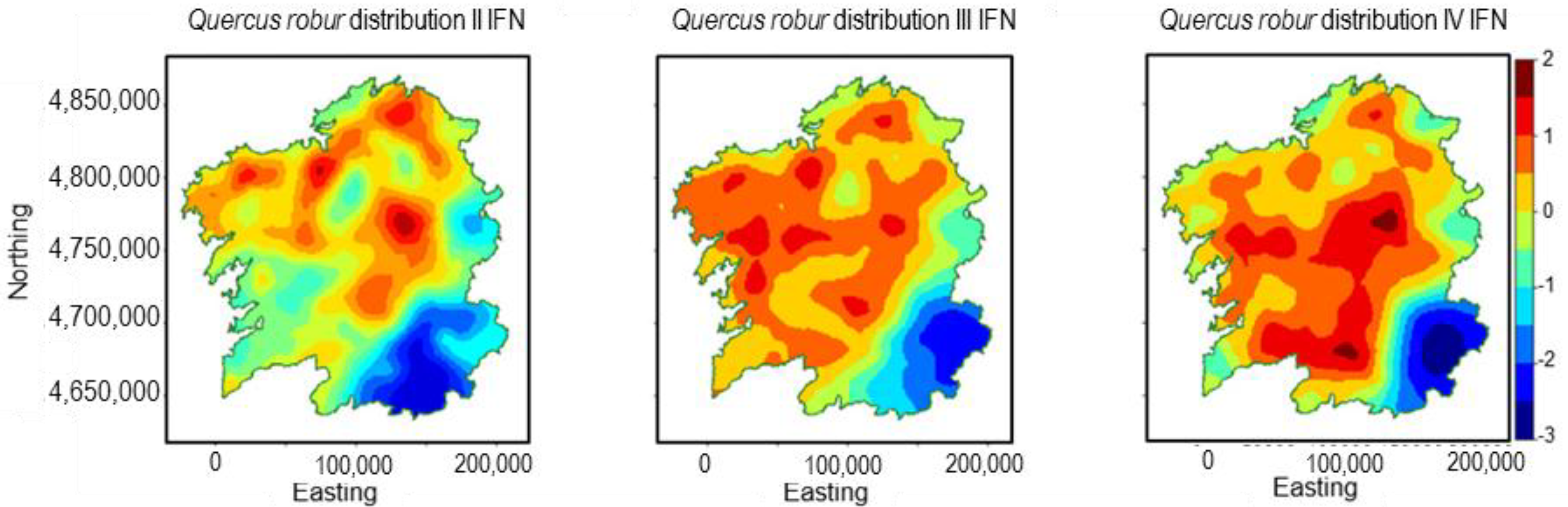
3.4. Quercus robur
3.5. Summary
4. Conclusions
Author Contributions
Funding
Conflicts of Interest
References
- Running, S.W.; Nemani, R.R.; Heinsch, F.A.; Zhao, M.; Reeves, M.; Hashimoto, H. A continuous satellite-derived measure of global terrestrial primary production. Bioscience 2004, 54, 547–560. [Google Scholar] [CrossRef]
- Boisvenue, C.; Running, S.W. Impacts of climate change on natural forest productivity–evidence since the middle of the 20th century. Glob. Chang. Biol. 2006, 12, 862–882. [Google Scholar] [CrossRef]
- Davis, M.B.; Shaw, R.G. Range shifts and adaptive responses to Quaternary climate change. Science 2001, 292, 673–679. [Google Scholar] [CrossRef] [PubMed]
- Parmesan, C.; Yohe, G. A globally coherent fingerprint of climate change impacts across natural systems. Nature 2003, 421, 37–42. [Google Scholar] [CrossRef] [PubMed]
- Bonan, G.B. Forests and climate change: Forcings, feedbacks, and the climate benefits of forests. Science 2008, 320, 1444–1449. [Google Scholar] [CrossRef] [PubMed]
- Adams, H.D.; Macalady, A.K.; Breshears, D.D.; Allen, C.D.; Stephenson, N.L.; Saleska, S.R.; Huxman, T.E.; McDowell, N.G. Climate-induced tree mortality: Earth system consequences. Eos 2010, 91, 153–154. [Google Scholar] [CrossRef]
- Schröter, D.; Cramer, W.; Leemans, R.; Prentice, I.C.; Araújo, M.B.; Arnell, N.W.; Bondeau, A.; Bugmann, H.; Carter, T.R.; Gracia, C.A.; et al. Ecosystem service supply and vulnerability to global change in Europe. Science 2005, 310, 1333–1337. [Google Scholar] [CrossRef] [PubMed]
- Lindner, M.; Maroschek, M.; Netherer, S.; Kremer, A.; Barbati, A.; Garcia-Gonzalo, J.; Seidl, R.; Delzon, S.; Corona, P.; Kolström, M.; et al. Climate change impacts, adaptive capacity, and vulnerability of European forest ecosystems. For. Ecol. Manag. 2010, 259, 698–709. [Google Scholar] [CrossRef]
- Spathelf, P.; van der Maaten, E.; van der Maaten-Theunissen, M.; Campioli, M.; Dobrowolska, D. Climate change impacts in European forests: The expert views of local observers. Ann. For. Sci. 2014, 71, 131–137. [Google Scholar] [CrossRef]
- de Rivera, O.R.; Blangiardo, M.; López-Quílez, A.; Martín-Sanz, I. Species distribution modelling through Bayesian hierarchical approach. Theor. Ecol. 2018. [Google Scholar] [CrossRef]
- Lindner, M.; Fitzgerald, J.B.; Zimmermann, N.E.; Reyer, C.; Delzon, S.; Maaten, E.; Schelhaas, M.J.; Lasch, P.; Eggers, J.; Maaten-Theunissen, M.; et al. Climate change and European forests: What do we know, what are the uncertainties, and what are the implications for forest management? J. Environ. Manag. 2014, 146, 69–83. [Google Scholar] [CrossRef] [PubMed]
- Hanewinkel, M.; Cullmann, D.A.; Schelhaas, M.J.; Nabuurs, G.J.; Zimmermann, N.E. Climate change may cause severe loss in the economic value of European forest land. Nat. Clim. Chang. 2013, 3, 203–207. [Google Scholar] [CrossRef]
- Maaten, E.; Hamann, A.; Maaten-Theunissen, M.; Bergsma, A.; Hengeveld, G.; Lammeren, R.; Mohren, F.; Nabuurs, G.J.; Terhürne, R.; Sterck, F. Species distribution models predict temporal but not spatial variation in forest growth. Ecol. Evol. 2017, 7, 2585–2594. [Google Scholar] [CrossRef] [PubMed] [Green Version]
- Elith, J.; Leathwick, J.R. Species distribution models: Ecological explanation and prediction across space and time. Ann. Rev. Ecol. Evol. Syst. 2009, 40, 677–697. [Google Scholar] [CrossRef]
- O’Neill, G.A.; Hamann, A.; Wang, T. Accounting for population variation improves estimates of the impact of climate change on species’ growth and distribution. J. Appl. Ecol. 2008, 45, 1040–1049. [Google Scholar] [CrossRef] [Green Version]
- Gray, L.K.; Hamann, A. Strategies for reforestation under uncertain future climates: Guidelines for Alberta, Canada. PLoS ONE 2011, 6, e22977. [Google Scholar] [CrossRef] [PubMed]
- Gray, L.K.; Hamann, A. Tracking suitable habitat for tree populations under climate change in western North America. Clim. Chang. 2013, 117, 289–303. [Google Scholar] [CrossRef]
- Hamann, A.; Aitken, S.N. Conservation planning under climate change: Accounting for adaptive potential and migration capacity in species distribution models. Divers. Distrib. 2013, 19, 268–280. [Google Scholar] [CrossRef]
- Schelhaas, M.J.; Nabuurs, G.J.; Hengeveld, G.; Reyer, C.; Hanewinkel, M.; Zimmermann, N.E.; Cullmann, D. Alternative forest management strategies to account for climate change-induced productivity and species suitability changes in Europe. Reg. Environ. Chang. 2015, 15, 1581–1594. [Google Scholar] [CrossRef] [Green Version]
- Hijmans, R.J.; Elith, J.; Species Distribution Modelling with R. The R Foundation for Statistical Computing. Available online: http://cran.r-project.org/ web/packages/dismo/vignettes/sdm.pdf (accessed on 5 May 2018).
- Simpson, D.; Lindgren, F.; Rue, H. Fast approximate inference with INLA: The past, the present and the future. arXiv, 2011; arXiv:1105.2982. [Google Scholar]
- Chakraborty, A.; Gelfand, A.E.; Wilson, A.M.; Latimer, A.M.; Silander, J.A., Jr. Modeling large scale species abundance with latent spatial processes. Ann. Appl. Stat. 2010, 4, 1403–1429. [Google Scholar] [CrossRef]
- Pressey, R.L.; Cabeza, M.; Watts, M.E.; Cowling, R.M.; Wilson, K.A. Conservation planning in a changing world. Trends Ecol. Evol. 2007, 22, 583–592. [Google Scholar] [CrossRef] [PubMed]
- Midgley, G.F.; Thuiller, W. Potential vulnerability of Namaqualand plant diversity to anthropogenic climate change. J. Arid Environ. 2007, 70, 615–628. [Google Scholar] [CrossRef]
- Loarie, S.R.; Carter, B.E.; Hayhoe, K.; McMahon, S.; Moe, R.; Knight, C.A.; Ackerly, D.D. Climate change and the future of California’s endemic flora. PLoS ONE 2008, 3, e2502. [Google Scholar] [CrossRef] [PubMed]
- Guisan, A.; Thuiller, W. Predicting species distribution: Offering more than simple habitat models. Ecol. Lett. 2005, 8, 993–1009. [Google Scholar] [CrossRef]
- Hijmans, R.J.; Graham, C.H. The ability of climate envelope models to predict the effect of climate change on species distributions. Glob. Chang. Biol. 2006, 12, 2272–2281. [Google Scholar] [CrossRef]
- Wisz, M.S.; Hijmans, R.J.; Li, J.; Peterson, A.T.; Graham, C.H.; Guisan, A. Effects of sample size on the performance of species distribution models. Divers. Distrib. 2008, 14, 763–773. [Google Scholar] [CrossRef]
- Rivera, Ó.R.; López-Quílez, A. Development and Comparison of Species Distribution Models for Forest Inventories. ISPRS Int. J. Geo-Inf. 2017, 6, 176. [Google Scholar] [CrossRef]
- Guisan, A.; Edwards, T.C.; Hastie, T. Generalized linear and generalized additive models in studies of species distributions: Setting the scene. Ecol. Model. 2002, 157, 89–100. [Google Scholar] [CrossRef]
- Busby, J. BIOCLIM—A bioclimate analysis and prediction system. Plant Prot. Q. (Aust.) 1991, 6, 64–68. [Google Scholar]
- Leathwick, J.R.; Rowe, D.; Richardson, J.; Elith, J.; Hastie, T. Using multivariate adaptive regression splines to predict the distributions of New Zealand’s freshwater diadromous fish. Freshw. Biol. 2005, 50, 2034–2052. [Google Scholar] [CrossRef]
- Munoz, F.; Pennino, M.G.; Conesa, D.; López-Quílez, A.; Bellido, J.M. Estimation and prediction of the spatial occurrence of fish species using Bayesian latent Gaussian models. Stoch. Environ. Res. Risk Assess. 2013, 27, 1171–1180. [Google Scholar] [CrossRef]
- Underwood, A.J. Techniques of analysis of variance in experimental marine biology and ecology. Oceanography and marine biology: An annual review. Ann. Rev. Oceanogr. Mar. Biol. 1981, 19, 513–605. [Google Scholar]
- Hurlbert, S.H. Pseudoreplication and the design of ecological field experiments. Ecol. Monogr. 1984, 54, 187–211. [Google Scholar] [CrossRef]
- Royle, J.A.; Kéry, M.; Gautier, R.; Schmid, H. Hierarchical spatial models of abundance and occurrence from imperfect survey data. Ecol. Monogr. 2007, 77, 465–481. [Google Scholar] [CrossRef]
- Cressie, N.; Calder, C.A.; Clark, J.S.; Hoef, J.M.V.; Wikle, C.K. Accounting for uncertainty in ecological analysis: The strengths and limitations of hierarchical statistical modeling. Ecol. Appl. 2009, 19, 553–570. [Google Scholar] [CrossRef] [PubMed]
- Gelfand, A.E.; Diggle, P.J.; Fuentes, M.; Guttorp, P. (Eds.) Handbook of Spatial Statistics; CRC Press: Boca Raton, FL, USA, 2010. [Google Scholar]
- Svenning, J.C.; Normand, S.; Kageyama, M. Glacial refugia of temperate trees in Europe: Insights from species distribution modelling. J. Ecol. 2008, 96, 1117–1127. [Google Scholar] [CrossRef]
- López Sáez, J.A.; López García, P.; López Merino, L. La transición Mesolítico-Neolítico en el Valle Medio del Ebro y en el Prepirineo aragonés desde una perspectiva paleoambiental: Dinámica de la antropización y origen de la agricultura. Rev. Iberoam. Hist. 2006, 1, 4–11. [Google Scholar]
- López Sáez, J.A.; López García, P.; López Merino, L. El impacto humano en la Cordillera Cantábrica: Estudios palinológicos durante el Holoceno medio. Zona Arqueol. 2006, 7, 122–131. [Google Scholar]
- López Sáez, J.A.; Galop, D.; Iriarte Chiapusso, M.J.; López Merino, L. Paleoambiente y antropización en los Pirineos de Navarra durante el Holoceno medio (VI–IV milenios cal. BC): Una perspectiva palinológica. Veleia 2008, 24–25, 645–653. [Google Scholar]
- Carrión, J.S.; Fuentes, N.; González-Sampériz, P.; Quirante, L.S.; Finlayson, J.C.; Fernández, S.; Andrade, A. Holocene environmental change in a montane region of southern Europe with a long history of human settlement. Quat. Sci. Rev. 2007, 26, 1455–1475. [Google Scholar] [CrossRef]
- Matejicek, L.; Vavrova, E.; Cudlin, P. Spatio-temporal modelling of ground vegetation development in mountain spruce forests. Ecol. Model. 2011, 222, 2584–2592. [Google Scholar] [CrossRef]
- Gratzer, G.; Canham, C.; Dieckmann, U.; Fischer, A.; Iwasa, Y.; Law, R.; Lexer, M.J.; Sandmann, H.; Spies, T.A.; Splechtna, B.E.; et al. Spatio-temporal development of forests–current trends in field methods and models. Oikos 2004, 107, 3–15. [Google Scholar] [CrossRef] [Green Version]
- O’Rourke, S.; Kelly, G.E. Spatio-temporal modelling of forest growth spanning 50 years—The effects of different thinning strategies. Procedia Environ. Sci. 2015, 26, 101–104. [Google Scholar] [CrossRef]
- Diggle, P.J. Statistical Analysis of Spatial Point Patterns; Arnold: London, UK, 2003. [Google Scholar]
- Stoyan, D.; Penttinen, A. Recent applications of point process methods in forestry statistics. Stat. Sci. 2000, 15, 61–78. [Google Scholar]
- Illian, J.; Penttinen, A.; Stoyan, H.; Stoyan, D. Statistical Analysis and Modelling of Spatial Point Patterns; John Wiley & Sons: Hoboken, NJ, USA, 2008; Volume 70. [Google Scholar]
- Grabarnik, P.; Särkkä, A. Modelling the spatial structure of forest stands by multivariate point processes with hierarchical interactions. Ecol. Model. 2009, 220, 1232–1240. [Google Scholar] [CrossRef]
- Cosandey-Godin, A.; Krainski, E.T.; Worm, B.; Flemming, J.M. Applying Bayesian spatiotemporal models to fisheries bycatch in the Canadian Arctic. Can. J. Fish. Aquat. Sci. 2014, 72, 186–197. [Google Scholar] [CrossRef]
- Wade, P.R. Bayesian methods in conservation biology. Conserv. Biol. 2000, 14, 1308–1316. [Google Scholar] [CrossRef]
- Wintle, B.A.; McCarthy, M.A.; Volinsky, C.T.; Kavanagh, R.P. The use of Bayesian model averaging to better represent uncertainty in ecological models. Conserv. Biol. 2003, 17, 1579–1590. [Google Scholar] [CrossRef]
- Illian, J.B.; Martino, S.; Sørbye, S.H.; Gallego-Fernández, J.B.; Zunzunegui, M.; Esquivias, M.P.; Travis, J.M. Fitting complex ecological point process models with integrated nested Laplace approximation. Methods Ecol. Evol. 2013, 4, 305–315. [Google Scholar] [CrossRef] [Green Version]
- Rue, H.; Martino, S. Approximate Bayesian inference for hierarchical Gaussian Markov random field models. J. Stat. Plan. Inference 2007, 137, 3177–3192. [Google Scholar] [CrossRef]
- Lindgren, F.; Rue, H.; Lindström, J. An explicit link between Gaussian fields and Gaussian Markov random fields: The stochastic partial differential equation approach. J. R. Stat. Soc. Ser. B 2011, 73, 423–498. [Google Scholar] [CrossRef]
- Rue, H.; Martino, S.; Chopin, N. Approximate Bayesian inference for latent Gaussian models by using integrated nested Laplace approximations. J. R. Stat. Soc. Ser. B 2009, 71, 319–392. [Google Scholar] [CrossRef] [Green Version]
- Beguin, J.; Martino, S.; Rue, H.; Cumming, S.G. Hierarchical analysis of spatially autocorrelated ecological data using integrated nested Laplace approximation. Methods Ecol. Evol. 2012, 3, 921–929. [Google Scholar] [CrossRef] [Green Version]
- Dutra Silva, L.; Brito de Azevedo, E.; Bento Elias, R.; Silva, L. Species Distribution Modeling: Comparison of Fixed and Mixed Effects Models Using INLA. ISPRS Int. J. Geo-Inf. 2017, 6, 391. [Google Scholar] [CrossRef]
- San-Miguel-Ayanz, J.; Rigo, D.D.; Caudullo, G.; Houston Durrant, T.; Mauri, A. European Atlas of Forest Tree Species; European Commission, Joint Research Centre: Brussels, Belgium, 2016. [Google Scholar]
- Herrera, S.; Gutiérrez, J.M.; Ancell, R.; Pons, M.R.; Frías, M.D.; Fernández, J. Development and analysis of a 50-year high-resolution daily gridded precipitation dataset over Spain (Spain02). Int. J. Climatol. 2012, 32, 74–85. [Google Scholar] [CrossRef] [Green Version]
- Herrera, S.; Fernández, J.; Gutiérrez, J.M. Update of the Spain02 gridded observational dataset for EURO-CORDEX evaluation: Assessing the effect of the interpolation methodology. Int. J. Climatol. 2016, 36, 900–908. [Google Scholar] [CrossRef]
- Gastón, A.; Soriano, C.; Gómez-Miguel, V. Lithologic data improve plant species distribution models based on coarse-grained occurrence data. For. Syst. 2009, 18, 42–49. [Google Scholar]
- Van Liedekerke, M.; Jones, A.; Panagos, P. ESDBv2 Raster Library—A Set of Rasters Derived from the European Soil Database Distribution v2.0; European Commission and the European Soil Bureau Network, CDROM, EUR, 19945; European Commission: Brussels, Belgium, 2006. [Google Scholar]
- Gelfand, A.E.; Silander, J.A.; Wu, S.; Latimer, A.; Lewis, P.O.; Rebelo, A.G.; Holder, M. Explaining species distribution patterns through hierarchical modeling. Bayesian Anal. 2006, 1, 41–92. [Google Scholar] [CrossRef]
- Blangiardo, M.; Cameletti, M. Spatial and Spatio-Temporal Bayesian Models with R-INLA; John Wiley & Sons: Hoboken, NJ, USA, 2015. [Google Scholar]
- Geisser, S.; Eddy, W.F. A predictive approach to model selection. J. Am. Stat. Assoc. 1979, 74, 153–160. [Google Scholar] [CrossRef]
- Vehtari, A.; Lampinen, J. Bayesian model assessment and comparison using cross-validation predictive densities. Neural Comput. 2002, 14, 2439–2468. [Google Scholar] [CrossRef] [PubMed]
- Gelman, A.; Shalizi, C.R. Philosophy and the practice of Bayesian statistics. Br. J. Math. Stat. Psychol. 2013, 66, 8–38. [Google Scholar] [CrossRef] [PubMed]
- Spiegelhalter, D.; Best, N.G.; Carlin, B.P.; Van der Linde, A. Bayesian measures of model complexity and fit. Qual. Control Appl. Stat. 2003, 48, 431–432. [Google Scholar] [CrossRef]
- Van Der Linde, A. DIC in variable selection. Stat. Neerl. 2005, 59, 45–56. [Google Scholar] [CrossRef]
- Watanabe, S. Asymptotic equivalence of Bayes cross validation and widely applicable information criterion in singular learning theory. J. Mach. Learn. Res. 2010, 11, 3571–3594. [Google Scholar]
- Li, L.; Qiu, S.; Zhang, B.; Feng, C.X. Approximating cross-validatory predictive evaluation in Bayesian latent variable models with integrated IS and WAIC. Stat. Comput. 2016, 26, 881–897. [Google Scholar] [CrossRef]
- Pettit, L.I. The conditional predictive ordinate for the normal distribution. J. R. Stat. Soc. Ser. B 1990, 52, 175–184. [Google Scholar]
- Gneiting, T.; Raftery, A.E. Strictly proper scoring rules, prediction, and estimation. J. Am. Stat. Assoc. 2007, 102, 359–378. [Google Scholar] [CrossRef]
- Roos, M.; Held, L. Sensitivity analysis in Bayesian generalized linear mixed models for binary data. Bayesian Anal. 2011, 6, 259–278. [Google Scholar] [CrossRef] [Green Version]
- Golding, N.; Purse, B.V. Fast and flexible Bayesian species distribution modelling using Gaussian processes. Methods Ecol. Evol. 2016, 7, 598–608. [Google Scholar] [CrossRef] [Green Version]
- Warton, D.I.; Blanchet, F.G.; O’Hara, R.B.; Ovaskainen, O.; Taskinen, S.; Walker, S.C.; Hui, F.K. So Many Variables: Joint Modeling in Community Ecology. Trends Ecol. Evol. 2015, 30, 766–779. [Google Scholar] [CrossRef] [PubMed]
- Redding, D.W.; Cunningham, A.A.; Woods, J.; Jones, K.E. Spatial and seasonal predictive models of Rift Valley Fever disease. Philos. Trans. R. Soc. Lond. B 2016, 372, 20160165. [Google Scholar] [CrossRef] [PubMed]
- Renner, I.W.; Warton, D.I. Equivalence of MAXENT and Poisson Point Process Models for Species Distribution Modeling in Ecology. Biometrics 2013, 69, 274–281. [Google Scholar] [CrossRef] [PubMed]


| Inventory | Abies alba Mill. | Castanea sativa Mill. | Pinus pinaster Ait. | Quercus robur L. |
|---|---|---|---|---|
| II (1980s) | 1% | 26% | 51% | 51% |
| III (1990s) | 2% | 15% | 38% | 40% |
| IV (2000s) | 1% | 35% | 46% | 59% |
| Abies alba | Castanea sativa | Pinus pinaster | Quercus robur | |||||
|---|---|---|---|---|---|---|---|---|
| Spatial | Spatio-Temporal | Spatial | Spatio-Temporal | Spatial | Spatio-Temporal | Spatial | Spatio-Temporal | |
| Elevation | − | − | Rn | Rn | + | + | + | + |
| Soil | Rn | Rn | Rn | Rn | Rn | Rn | Rn | − |
| Precipitation | − | − | Rn | Rn | Rn | + | Rn | − |
| Temperature | − | − | Rn | Rn | Rn | + | Rn | − |
| Max. Temperature | − | − | Rn | − | Rn | − | Rn | Rn |
| Min. Temperature | − | − | Rn | − | Rn | − | Rn | − |
| Abies alba | Castanea sativa | Pinus pinaster | Quercus robur | |||||
|---|---|---|---|---|---|---|---|---|
| Spatial | Spatio-Temporal | Spatial | Spatio-Temporal | Spatial | Spatio-Temporal | Spatial | Spatio-Temporal | |
| WAIC | 15.54 | 12.73 | 5.435 | 10.629 | 4.621 | 3.385 | 9.676 | 1.837 |
| LCPO | 1.531 | 1.251 | 2.327 | 2.986 | 3.725 | 2.327 | 2.382 | 1.965 |
© 2018 by the authors. Licensee MDPI, Basel, Switzerland. This article is an open access article distributed under the terms and conditions of the Creative Commons Attribution (CC BY) license (http://creativecommons.org/licenses/by/4.0/).
Share and Cite
Rodríguez de Rivera, Ó.; López-Quílez, A.; Blangiardo, M. Assessing the Spatial and Spatio-Temporal Distribution of Forest Species via Bayesian Hierarchical Modeling. Forests 2018, 9, 573. https://doi.org/10.3390/f9090573
Rodríguez de Rivera Ó, López-Quílez A, Blangiardo M. Assessing the Spatial and Spatio-Temporal Distribution of Forest Species via Bayesian Hierarchical Modeling. Forests. 2018; 9(9):573. https://doi.org/10.3390/f9090573
Chicago/Turabian StyleRodríguez de Rivera, Óscar, Antonio López-Quílez, and Marta Blangiardo. 2018. "Assessing the Spatial and Spatio-Temporal Distribution of Forest Species via Bayesian Hierarchical Modeling" Forests 9, no. 9: 573. https://doi.org/10.3390/f9090573
APA StyleRodríguez de Rivera, Ó., López-Quílez, A., & Blangiardo, M. (2018). Assessing the Spatial and Spatio-Temporal Distribution of Forest Species via Bayesian Hierarchical Modeling. Forests, 9(9), 573. https://doi.org/10.3390/f9090573