Generalized Nonlinear Mixed-Effects Individual Tree Crown Ratio Models for Norway Spruce and European Beech

Abstract

Tree crowns are commonly measured to understand tree growth and stand dynamics. Crown ratio (CR—crown depth-to-total height ratio) is significantly affected by a number of tree- and stand-level characteristics and other factors as well. Generalized mixed-effects CR models were developed using a large dataset (measurements from 14,669 trees of Norway spruce (Picea abies (L.) Karst.) and European beech (Fagus sylvatica (L.)) acquired from permanent research plots in various parts of the Czech Republic. Among several tree- and stand-level variables evaluated, diameter at breast height, height to crown base, dominant height, basal area of trees larger in diameter than a focal tree, relative spacing index, and variables describing the effects of species mixture and canopy height differentiation significantly contributed to CR variation. We included sample-plot-level variations caused by randomness in the data and other stochastic factors into the CR models using the mixed-effects modeling approach. The logistic function, which predicts the values between 0 and 1, was chosen to develop the generalized CR mixed-effects model. A large proportion of the CR variation (R²_adj ≈ 0.63 (Norway spruce); 0.72 (European beech)) was described by generalized mixed-effects model without significant residual trends. Testing the CR model against a part of the model fitting dataset confirmed its high prediction precision. Our CR model can be useful for growth simulation using inventory databases that lack crown measures. Other potential implications of our CR models in forest management are mentioned in the article.

1. Introduction

The crown is characterized by crown length, crown width, crown density, leaf area, and crown ratio (CR). The crown manufactures the photosynthetic materials and supplies to other parts of a tree, and therefore these parts are closely related to crown sizes (crown depth, crown width, crown fullness). Specifically, tree crowns play crucial roles in regulating solar energy, recycling nutrients, distributing precipitation, and retaining moisture in the forest stands. The crown size is a good indicator of general health and vigor of a tree [1,2,3]. For example, trees with large and dense crowns have vigorous growth, while trees with small and sparse crowns have little or no growth. Measurements of the crown dimensions are often used to evaluate health, growth, and production efficiency of trees and forest stands [3,4,5].

The crown measures are often used for modeling distribution of the solar radiation, water and nutrient within trees, and modeling growth of trees [3,6]. Research on the crown measures including CR contributes to the knowledge on ecosystem productivity and biodiversity [7]. As a good indicator of tree health and vigor [1,3,8,9], CR is used to determine the thinning intensity and its potential response of the residual trees within a stand [10]. The CR can be used as an indirect measure of the photosynthetic ability of trees and their competitive interactions [10,11]. The CR is used to assess wood quality [12,13] and wind firmness [14] of trees. The potential growth of a tree is determined by surface area or volume of tree foliage. However, these attributes cannot be measured directly; instead, CR or crown depth can be used as an appropriate substitute in the growth and yield models [15]. The crown measures including CR are often included as predictor variables into a number of forest models, such as growth models [16,17,18,19,20,21,22,23,24], survival analysis and mortality models [25,26], biomass models [27,28,29], and stem taper and volume models [30,31,32]. The CR can be used to assess canopy density [33], potentiality of wildlife habitat and recreation [34,35] and risk of forest fires [36], and to model light interception through canopies [37,38].

Considering the necessity of the crown models for decision-making in forestry, a number of studies that involved tree-based crown models have been carried out, including crown diameter models [39,40,41,42,43,44], crown shape models [45], crown rise models [46], crown spread ratio models [47], crown projection ratio models [48], and crown ratio models [8,49,50,51,52,53]. The CR models are much more important than any other models of the crown measures for forest management [8,24]. Therefore, developing a precise species-specific CR model is necessary, which may be challenging, but possible with the use of a comprehensive and extensive dataset and application of a robust modeling method (mixed-effects modeling). Except for two existing CR modeling studies [20,53], all other studies have used the ordinary least square regression method—also known as the traditional regression method. This is not appropriate for modeling tree- or stand-level characteristics using the measurements taken from the same sampling unit, because measurements from the same sampling unit are most likely correlated to each other. In this situation, the mixed-effects modeling approach, which allows to include both fixed and random effects into the model, may be the most appropriate [54]. The fixed parameters in the mixed-effects model account for the effects of main and covariate predictors as in the ordinary least square regression, while the random component accounts for variability caused by stochastic factors [41,53,54,55,56,57].

Most of the existing CR models have included the measures describing the effects of competition (e.g., stand basal area, crown competition factor, and spacing index), the effects of size of trees (e.g., diameter, height, height-to-diameter ratio, and stand age), and the effects of site characteristics (e.g., altitude, slope, and aspect), but not the measures that describe the effects of intra- or inter-species interactions and canopy height differentiation on the CR variation. The effects of species mixture on tree and stand characteristics have been thoroughly analyzed in several studies [42,44,48,56,58,59,60]. These studies confirm that species-mixing effect on tree characteristics is highly significant; therefore, this cannot be disregarded when measurements from mixed stands are used. Like the tree height-to-diameter ratio [61,62] and crown projection ratio [48], the forms and sizes of crowns vary from tree to tree, depending on their associated canopies and social positions [3]. However, none of the existing CR models has used the predictors that describe the effects of species mixture and canopy height differentiation on CR. Furthermore, except for the CR models by Hasenauer and Monserud [8], which were developed using the traditional regression method without considering the effects of species mixture and canopy height differentiation, no study has sought to develop a generalized (composite) mixed-effects CR model for Norway spruce and European beech—the most important species in Europe.

The objective of this study is to evaluate the hypothesis, through application of a mixed-effects modeling approach, whether the effects of intra- or inter-species interaction and canopy height differentiation on CR are significant. Moreover, the effects of spacing, site quality, stand development stage, and social positions of trees on the relationship between diameter and CR were also investigated. A large dataset originating from research sample plots in various parts of the Czech Republic was used. It is concluded that the proposed CR models are useful for tree growth simulations using inventory databases that lack CR data.

2. Materials and Methods

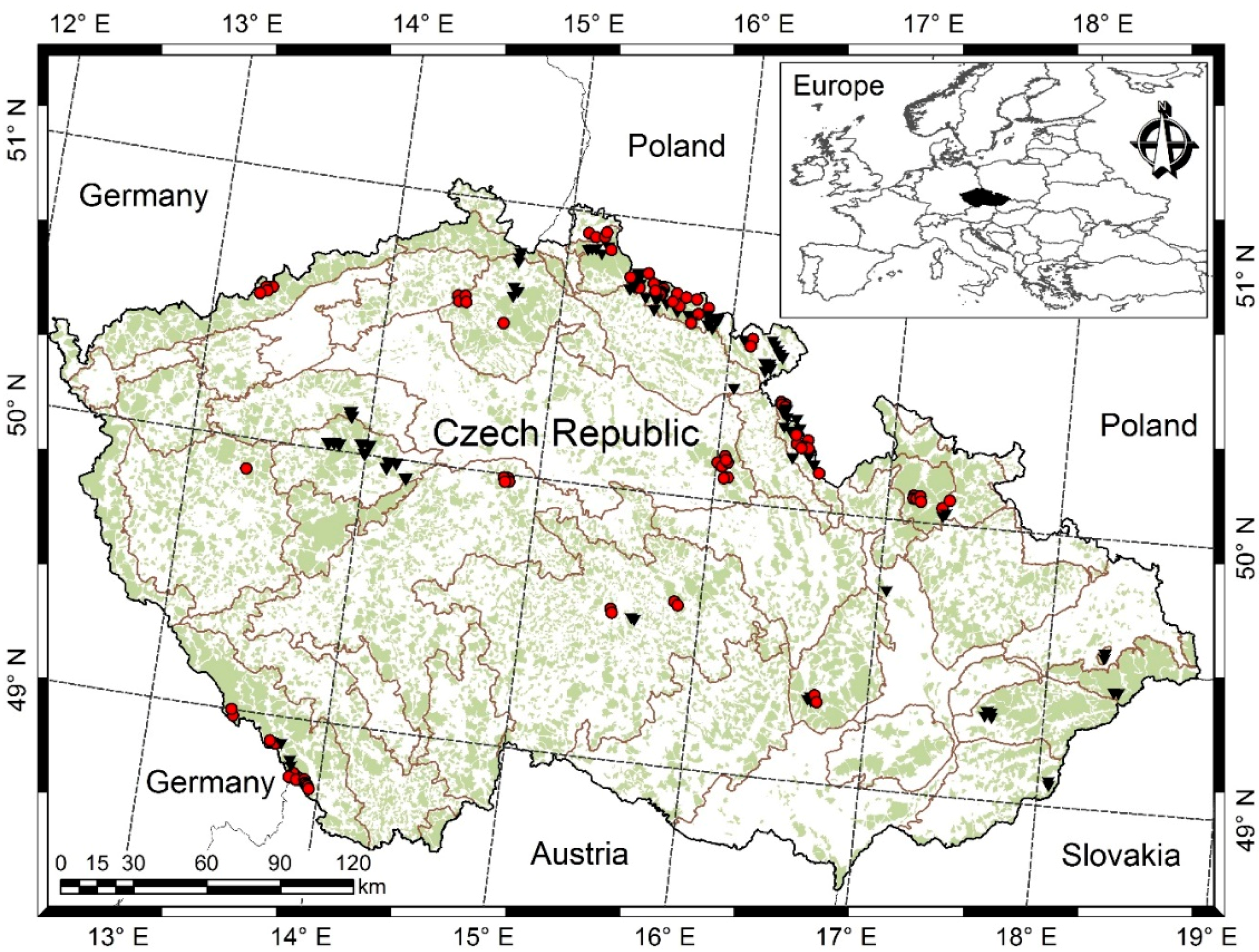
2.1. Sampling and Measurements

We collected data from permanent research plots, hereafter termed as sample plots, which are distributed across the 26 Natural Forest Areas of the Czech Republic (Figure 1). The studied forests consist of the monospecific stands and mixed stands of Norway spruce and European beech. Most of these sample plot data have been used in other studies [42,48,56,61,63,64] with different objectives. Therefore, more information about sample plots and sampling designs can be obtained from this literature. Area of the sample plots varies from 2500 to 4900 m², and they have square and rectangular shapes. The sample plots are representative of a wide range of altitudes (240–1370 m), temperatures (4–9.5 °C of mean annual temperature), precipitation (500–1450 mm of mean annual precipitation), and growing periods (45–180 days of growing season length) [48,56]. The canopy layers, mortality, regeneration, dead wood stocking, stand density, and stand development stage were taken into account while laying out the sample plots [65]. Our data therefore represent a wide range of stand conditions, environmental variabilities, and management regimes. The majority of the stands, especially those of beech, originated from spontaneous development, and about 20% spruce stands were from plantation. About 80% of stands were left for natural regeneration, with stand ages varying from 10 to 150 years, and management intervention involved sanitary cutting (e.g., extraction of bark beetle- and disease-affected trees and low harvesting [48]). The rest of the stands were managed by focusing on the cutting of trees by a shelter wood selection system, with creation of 5% canopy gaps. Sample plots heavily damaged by air pollution, windbreak, bark beetles, and diseases [66,67] were excluded from our study.

The Forest Management Institute has developed protocols for sample plot inventory [68]. We followed such protocols and conducted the inventory through April 2007 and May 2016. No repeated measurement was carried out, meaning that our dataset lacks the temporal variability. We measured the over bark diameter at breast height (DBH, 1.3 m above ground) using a caliper (precision 1 mm) and total height by a Laser Vertex hypsometer (Haglöf, Långsele, Sweden) that has 10 cm precision. Height to crown base (HCB) was measured for all individuals with DBH ≥2.5 cm and total height ≥1.5 m on each sample plot. We considered HCB as the lowest point of the crown on the bole where continuous whorl with all living branches was formed. However, we did not consider a whorl as a continuous if there were one or more dead whorls above it [48,56]. We recorded 1–26 species per sample plot.

2.2. Data Analysis

2.2.1. Tree and Stand Measures

Site quality, stand development stage, and stand density or competition may have significant effects on the crown of trees [8,40,41,42,43,44,49,69]. Considering this, we evaluated several tree and stand measures for their potential contributions to the CR variation. The site index, which best describes site quality, is included as one of the predictors into various forest models [70,71]. However, due to lack of this information, we did not include site index into our CR model. The dominant height (HDOM), which is assumed to describe the combined effect of site quality and stand development stage, was included into our CR model. The field crew did not identify dominant trees, but we identified them from measured sample height trees by applying the methods suggested by Sharma et al. [42,72]. We then computed the HDOM and dominant diameter (DDOM) for each sample plot according to the definition of HDOM, i.e., 100 largest trees per hectare [73]. We also computed other important stand measures, such as stem number per hectare (N, ha⁻¹), DBH sum of all individuals (DBHSUM, cm), stand basal area (BA, m² ha⁻¹), arithmetic mean DBH (AMD, cm), and quadratic mean DBH (QMD, cm). We also calculated the relative spacing index (RSI), which is defined by $\mathrm{RSI}=\sqrt{\mathrm{10,000}/\mathrm{N}}/\mathrm{HDOM}$ [11,20,74,75]. We assumed RSI as an effective stand density measure for determining the thinning specification, because it includes stocking and combined effect of site quality and stand development stage through N and HDOM, respectively [11,44,76].

We also computed the measures describing competitive interactions among the individual trees, such as basal area of trees larger in diameter than a subject tree (BAL) and ratio of DBH to QMD (dq). All tree- and stand-level competition measures were computed using the measurements regardless of species. There can be a significant effect of species mixture on tree growth and stand dynamics [44,48,56,58,59,60]. We also included a variable (basal area proportion of the species of interest: BAPRO) that describes species mixing effect on the CR variation.

We excluded trees with missing measurements of total height or HCB and other tree variables. The final dataset is summarized in

Table 1. Summary statistics of data.

Variables	Mean ± Std. (Range)
	Norway Spruce	European Beech
Number of sample plots	90 (18 monospecific + 72 mixed species)	88 (18 monospecific + 70 mixed species)
Number of sample trees	6736	7933
Number of trees per sample plot	149 ± 115 (3–430)	142 ± 124 (3–515)
Number of trees per hectare (N ha−1)	1005 ± 676 (92–2568)	827 ± 745 (41–2568)
Basal area (BA, m2 ha−1)	47.2 ± 19.4 (7.2–91.4)	43.3 ± 14 (0.7–89.1)
BA proportion of a species (BAPRO)	0.72 ± 0.31 (0.0005–1)	0.72 ± 0.24 (0.0004–1)
BA of trees larger in diameter than a subject tree (BAL, m2 ha−1)	36.7 ± 21.2 (0–88.8)	33.9 ± 16.7 (0–86.3)
Quadratic mean DBH (QMD, cm)	28.9 ± 9.6 (11.9–60.4)	32.9 ± 11.8 (15.4–87.4)
DBH-to-QMD ratio (dq)	1.2 ± 0.5 (0.1–6.8)	1.1 ± 0.64 (0.12–5.7)
Arithmetic mean DBH (cm)	24.8 ± 10.5 (9.4–53.9)	28.6 ± 12.8 (9.4–84.4)
DBH sum (DBHSUM, cm)	4845 ± 1860 (813–9333)	4172 ± 1911 (675–9333)
Dominant diameter (DDOM, cm)	49.9 ± 13.3 (18.4–77.1)	56.7 ± 11.2 (24.7–84.3)
Dominant height (HDOM, m)	27.1 ± 8.2 (8–42)	30.6 ± 6.3 (13.6–42.8)
Mean height (m)	16.2 ± 6.7 (4.6–37.4)	19.2 ± 7.9 (6.6–42.8)
Relative spacing index (RSI)	0.15 ± 0.07 (0.05–0.44)	0.15 ± 0.06 (0.06–0.41)
Total height (m)	16.9 ± 9.9 (1.5–48.7)	19.4 ± 10.3 (1.5–50.6)
Diameter at breast height (DBH, cm)	26.7 ± 18.5 (2.5–119)	28.3 ± 20.1 (2.9–118.7)
Height-to-DBH ratio (HDR, m cm−1)	0.6 ± 0.3 (0.03–6.6)	0.8 ± 0.3 (0.1–6.1)
Height to crown base (HCB, m)	6.26 ± 5.7 (0.01–37)	8.5 ± 6.4 (0.1–35)
Crown diameter (CW, m)	3.7 ± 1.6 (0.5–13.9)	6.1 ± 3.2 (0.8–24.1)
Crown depth (CL, m)	10.6 ± 6.7 (0.2–35.3)	10.9 ± 6.4 (0.5–45.2)
Crown ratio (CR)	0.65 ± 0.19 (0.05–0.99)	0.58 ± 0.18 (0.05–0.99)

. We considered those stands as monospecific ones, where individuals other than species of interest with DBH 4 cm existed. The inventory crew did not differentiate trees by canopy height class (CC), i.e., suppressed, intermediate, and dominant in inventory. We applied the same approach, which was applied by Sharma et al. [48,61] for canopy height classification, as follows:

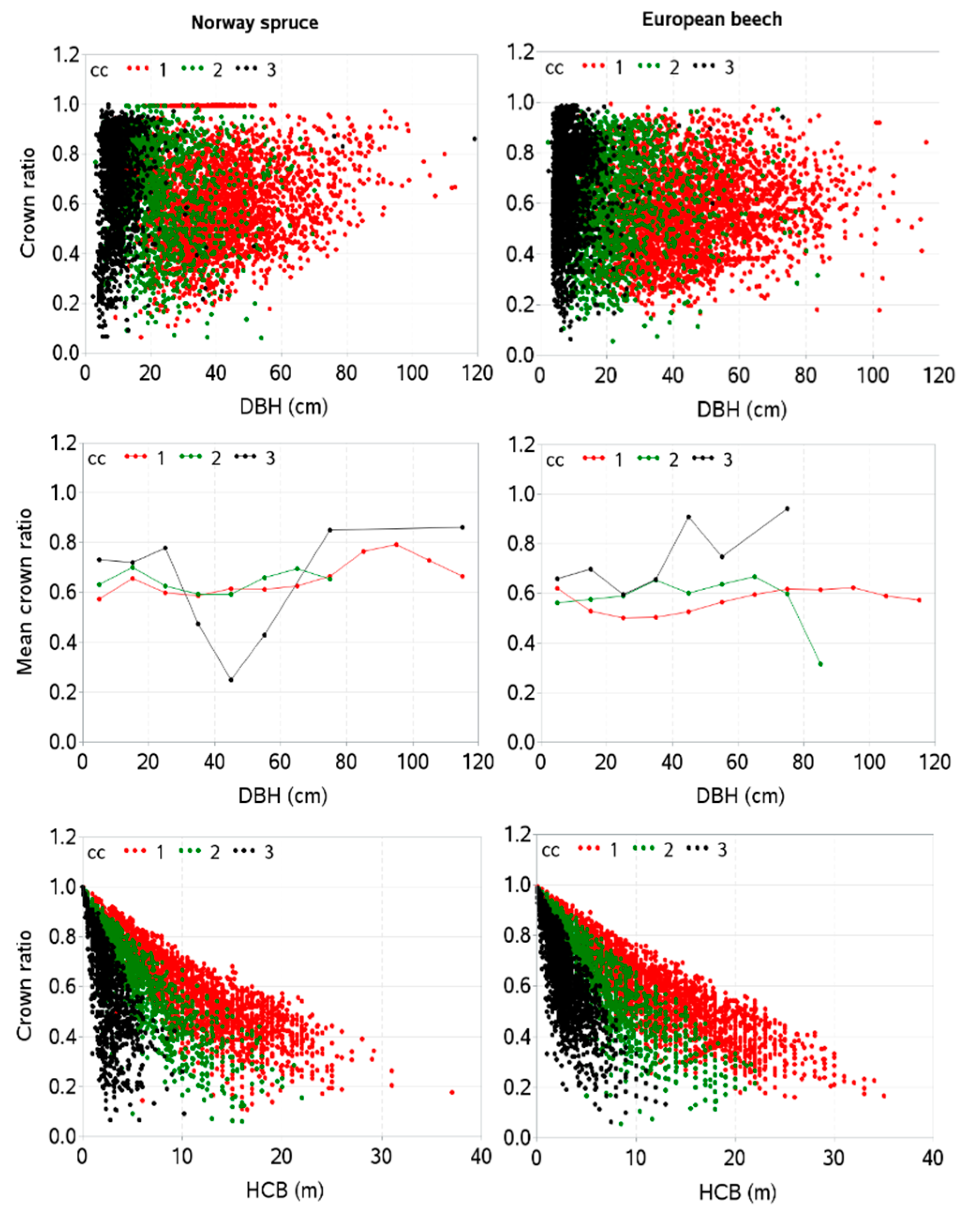
• canopy height class I, CC₁: height greater than 66% of the tallest tree;
• canopy height class II, CC₂: height between 33% and 66% of the tallest tree; and
• canopy height class III, CC₃: height less than 33% of the tallest tree.

Measurements of height of all living trees, irrespective of the species of interest on each sample plot allowed us to apply this classification approach. This classification has also resulted in a significant variability in the slenderness coefficient (height-diameter ratio) and crown projection ratio of trees between canopy height classes [48,61]. Graphs of CR against DBH and HCB by canopy height class are presented in Figure 2. This figure depicts that CR for any DBH or HCB of a given canopy height class is substantially different, so we included a variable describing the effect of canopy height differentiation into our CR models.

2.2.2. Model Development

Theoretically, values of CR should fall between 0 and 1, and considering this, we used only those functions [49,53], which predict CR between 0 and 1, to fit the data using DBH as a single predictor and compared fitting performances. The best fitted function was then used to include additional tree- and stand-level variables that describe tree size effect, combined effect of site quality and stand development stage, competition effect, species mixture effect, effect of canopy height differentiation, and component describing random effects on the CR variation. Among the 10 functions considered in preliminary analyses, a logistic function of the following form (Equation (1), henceforth termed as a base model) best fitted to the data:

$${\mathrm{CR}}_{ij}=\frac{1}{1+exp\left(-b_1{\mathrm{DBH}}_{ij}^{b_2}\right)}+{\epsilon }_{ij}$$

(1)

where CR_ij and DBH_ij are crown ratio and diameter at breast height (cm) of the jth tree on the ith sample plot, respectively, b₁ and b₂ are parameters to be estimated, and ε_ij is an error term.

We evaluated several tree- and stand-level variables (Table 1) for their potential contributions to the fitting improvement of the CR models. Evaluation was based on examination of graphs and correlation statistics [42,56,77]. The interaction effects between predictors and their transformations were also evaluated. Among several predictors evaluated, significantly highly contributing ones identified are HCB, HDOM, BAL, RSI, and BAPRO. The two-stage variable selection method [48,55,78] was applied to identify these predictors. This method entailed that a base model (Equation (1)) was fitted by sample plot, and scattered-matrix graphs of the estimated parameter values plotted against each of the predictors (Table 1) were examined. Since graphs of b₁ of a base model, plotted against HDOM, BAL, BAPRO, RSI, and HCB, showed strong correlation, we defined b₁ as a function of these variables and incorporated into the CR model. The variance influence factor, which is commonly used to assess the multi-collinearity among predictors [79], was used to check the dependency among those five selected predictors. Introducing many variables into the CR models may increase the fitting improvement, but this was not done, because this would cause over-parameterization, leading to the biased parameter and variance estimates [79]. The effects on the CR variation caused by canopy height differentiation were also included through application of the dummy variable modeling approach. Since b₁ of a base model (Equation (1)) was found more correlated to covariate predictors, this parameter was defined as a linear function of all five covariate predictors and three dummy variables describing canopy height classes.

The mixed-effects CR model was formulated through random effects inclusion (Equation (2)). This was necessary, because the global model (model without random effects) assumes no CR invariability exists within- and between-sample plots, which is not true [41,54,55,80]. Formulation details of any nonlinear mixed-effects model are found in the standard textbooks [54], so we present our final mixed-effects CR model here (Equation (2)):

$${\mathrm{CR}}_{ij}=\frac{1}{1+exp\left[-\left(b_1+u_{i1}\right){\mathrm{DBH}}_{ij}^{\left(b_2+u_{i2}\right)}\right]}+{\epsilon }_{ij}$$

(2)

$$\mathrm{with}{b}_1={\alpha }_1{z}_1+{\alpha }_2{z}_2+{\alpha }_3{z}_3+{\beta }_1{x}_1+{\beta }_2{x}_2+{\beta }_3{x}_3+{\beta }_4{x}_4+{\beta }_5{x}_5$$

where z_k is canopy height class CC_k (k = 1, 2, 3) (when a CR of a tree belongs to the kth canopy class then z_k = 1, otherwise 0); x₁ = HDOM_i; x₂ = BAL_i; x₃ = RSI_i; x₄ = BAPRO_i; x₅ = HCB_ij; variables HDOM_i,BAL_i, RSI_i, BAPRO_i, and HCB_ij are dominant height (m), basal area of trees larger than the jth subject tree (m² ha⁻¹), relative spacing index; basal area proportion of the species of interest, height to crown base of the jth tree (m) on the ith sample plot, respectively; α_i (i = 1, ..., 3) and β_i (i = 1, …, 5) are parameters to be estimated; ε_ij is an error term. In this equation, error vector and random effect vector were defined by ${\mathit{\epsilon }}_{\mathit{i}}\sim \mathit{N}\left(\mathbf{0},\mathit{R}\right)\mathrm{and}{\mathit{u}}_{\mathit{i}}\sim \mathit{N}\left(\mathbf{0},\mathit{D}\right),$ respectively. This means that error vector ε_i was assumed to have a normal distribution with zero mean and within-plot variance-covariance matrix R, which is given by Equation (3):

$${\mathit{R}}_{\mathit{i}}={\sigma }^2{\mathit{G}}_{\mathit{i}}^{\mathbf{0.5}}{\mathbf{\Gamma }}_{\mathit{i}}{\mathit{G}}_{\mathit{i}}^{\mathbf{0.5}}$$

(3)

A random effect vector u_i was assumed to have normal distribution with zero mean and within-plot variance-covariance matrix D, which is given by Equation (4).

$$\mathit{D}=\left[\begin{array}{cc}{\sigma }_{ui1}^2& {\sigma }_{ui1ui2}\\ {\sigma }_{ui2ui1}& {\sigma }_{ui2}^2\end{array}\right]$$

(4)

In Equation (3), σ² is an error dispersion [81], and this is equivalent to the residual variance and common to all sample plots. The matrix G_i accounts for within-sample plot variance heteroscedasticity and its elements are provided by a variance function. The matrix Γ_i accounts for within-plot error autocorrelations, but we assumed this matrix as an identity matrix, because our data lacked repeated measurements.

We detected the heteroscedasticity in our preliminary analyses even after the random effects were included into the CR model. We then evaluated three variance functions [41,54] for their heteroscedasticity reducing performances. According to the Akaike information criterion, a power function (Equation (5)) was found the most effective for heteroscedasticity reduction.

$$var\left({\epsilon }_{ij}\right)={\sigma }^2{\mathrm{DBH}}_{ij}^{2\varphi }$$

(5)

where $\varphi$ is a variance parameter to be estimated, and σ² is the same as in Equation (3).

2.3. Estimation of Model Parameters and Evaluation

The nonlinear mixed-effects models were estimated with the restricted maximum likelihood in SAS macro NLINMIX [82] by applying the expansion-around-zero method [83], and all base models were estimated with PROC NLIN in SAS [82]. The estimated model variants were evaluated using root mean square error (RMSE), adjusted coefficient of determination (R²_adj) [79], and Akaike information criterion (AIC) [84,85]. We also examined graphs of the residuals plotted against each of the predictors, and CR curves produced with estimated models. We used a 1% significance level in all analyses. Even though validating models with an external dataset provides credibility of predictions, we were unable to do this due to the unavailability of this dataset. We did not split the dataset to make the cross validation either, as this does not provide additional information on the fit statistics obtained from the model fitted using the entire dataset [86,87,88]. We used a part of the same fitting dataset to calibrate (localize) the mixed-effects CR models by applying the empirical best linear unbiased prediction (EBLUP) method [54].

2.4. The Localizing Mixed-Effects Model and Subject-Specific CR Prediction

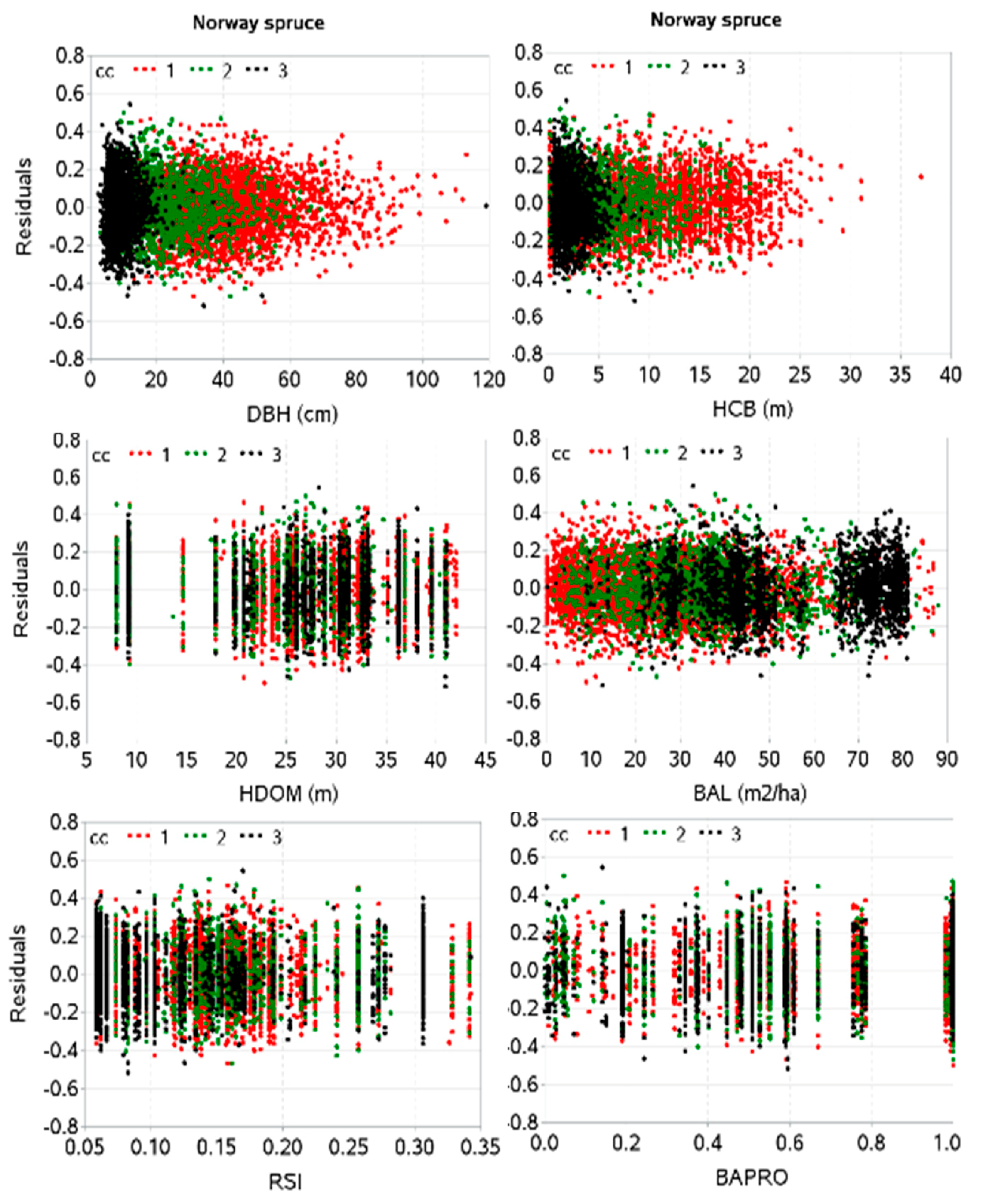
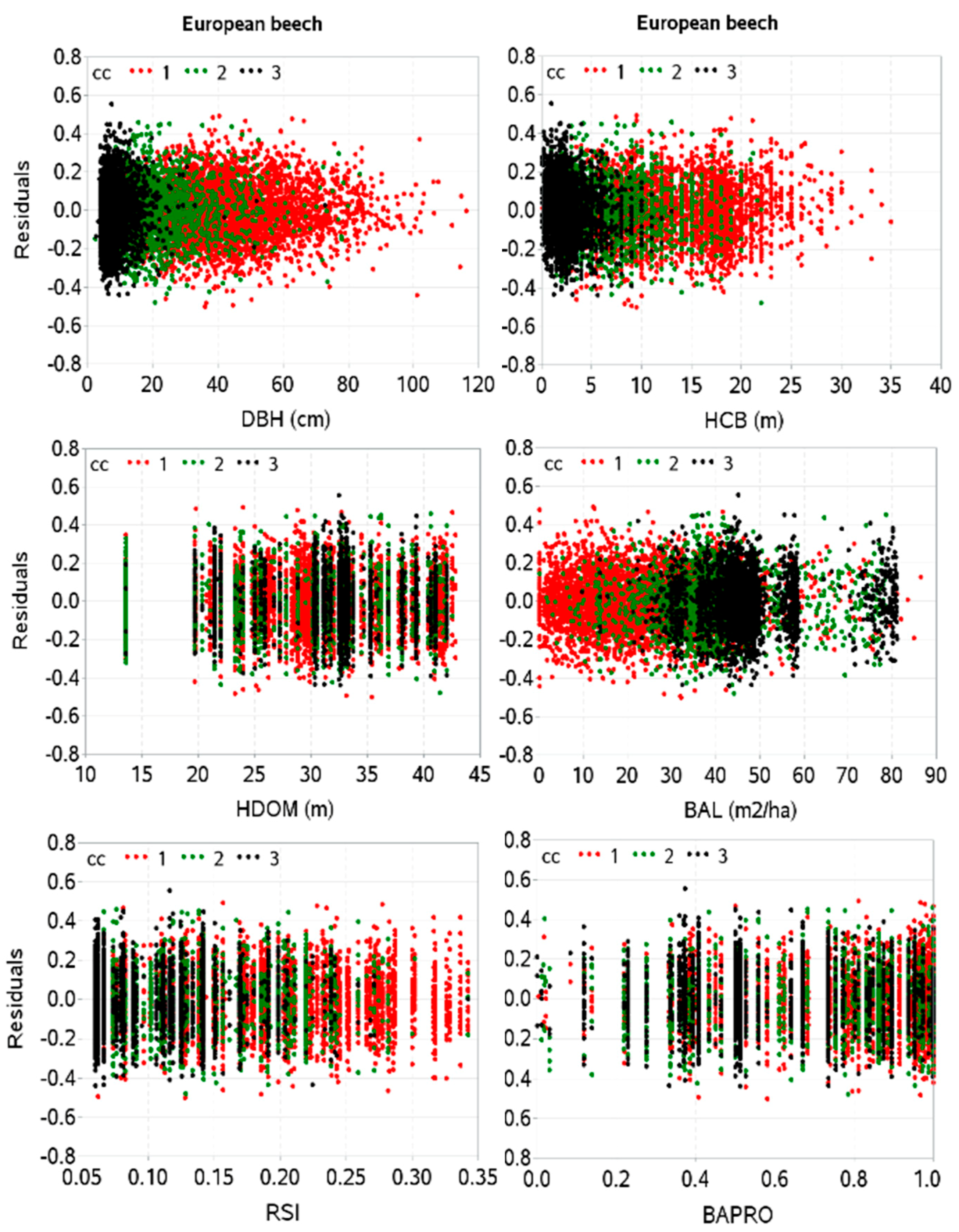
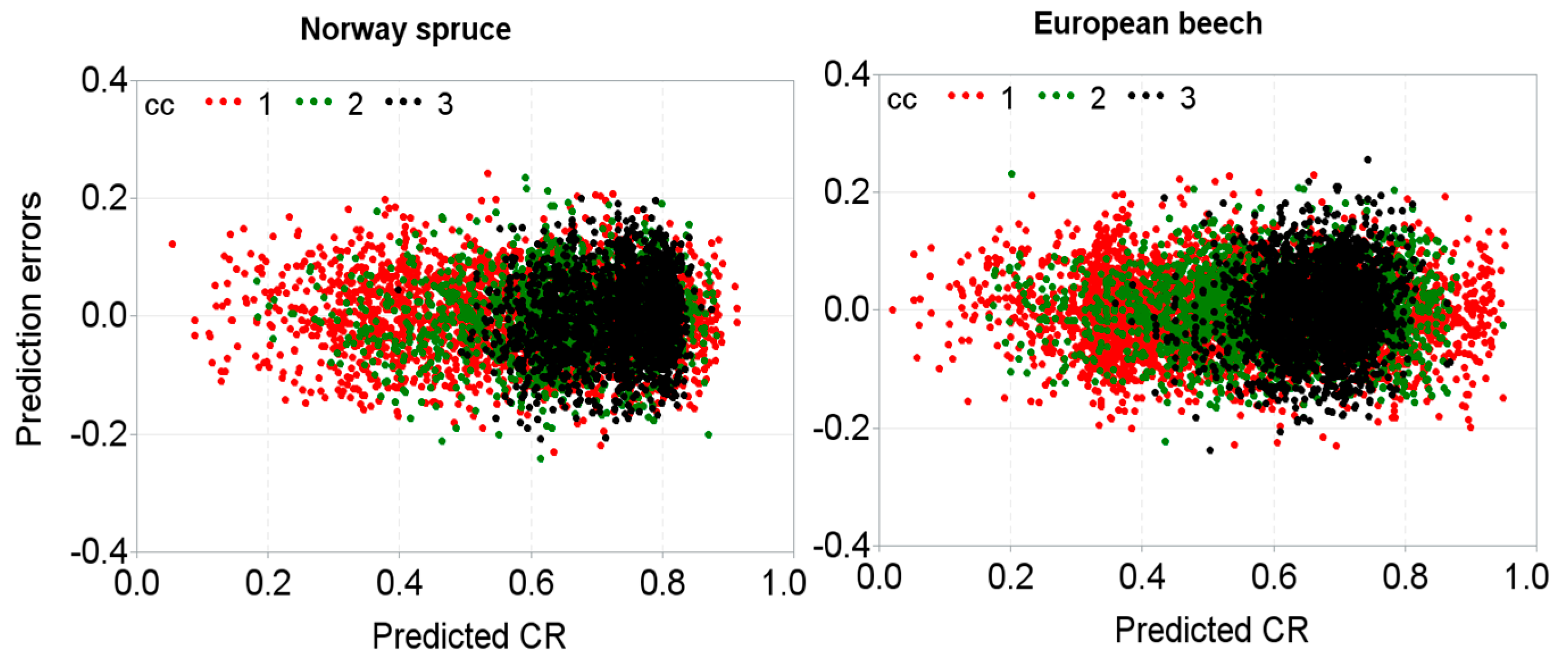
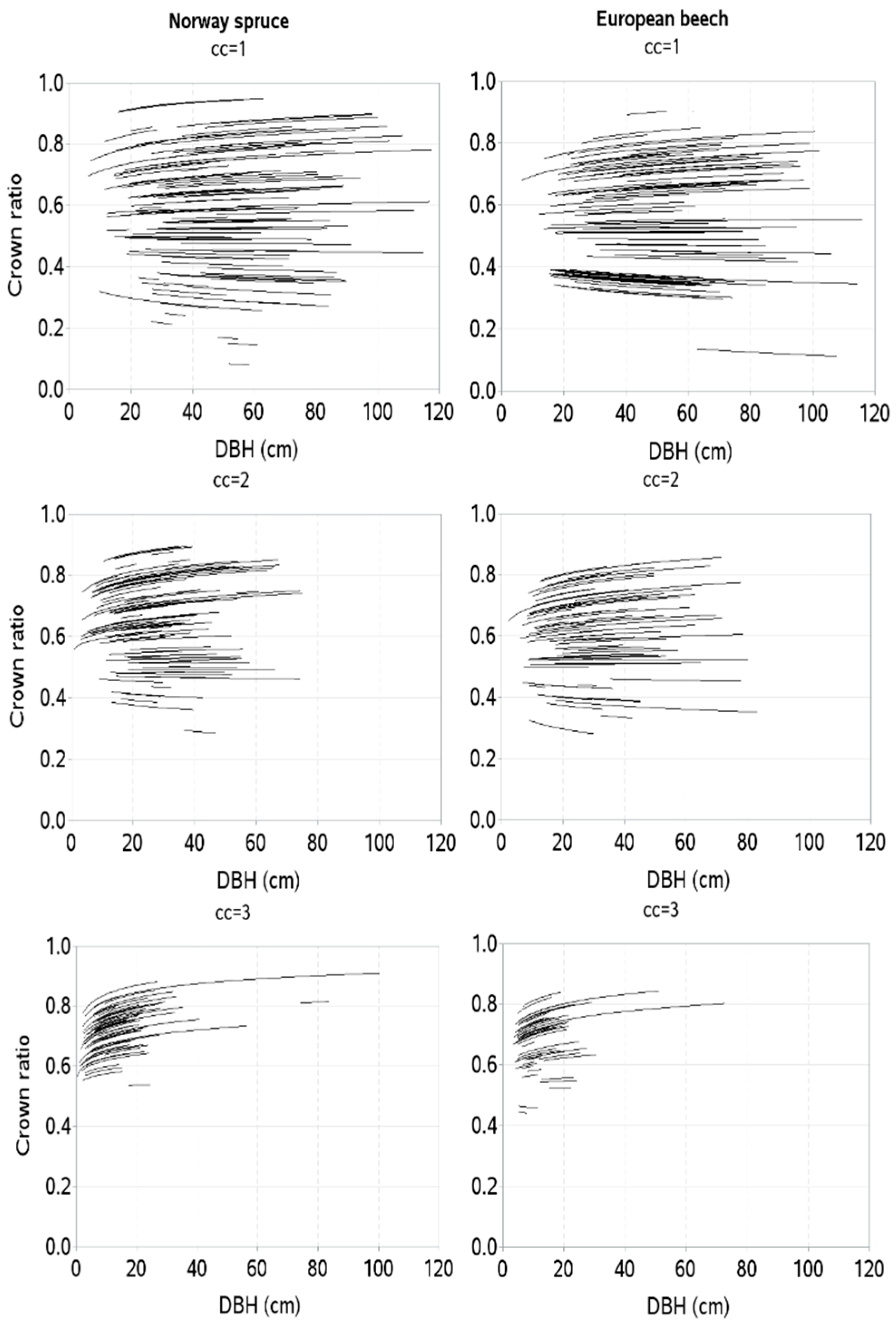
The prediction of CR could be made with or without calibrating the mixed-effects CR models. A prediction using estimated random effects requires a prior measurement of a response variable (CR) for a sub-sample of Norway spruce or European beech trees on each sample plot. The literature indicates that a sub-sample of four or five randomly selected trees per sample plot can be adequate for unbiased prediction [41,43,44,53,56,80,89]. We evaluated the predictive performance of our model through its calibration using a sub-sample of four randomly selected trees in a part of the model fitting dataset. For this, we selected only those sample plots, where at least five trees with measured HCB and total height of the species of interest were available. We estimated the random effects for each sample plot using the following EBLUP equation, which we implemented in PROC IML of SAS [82].

$${\mathit{u}}_{\mathit{i}}=\mathit{D}{\mathit{Z}}_i^T{\left({\mathit{Z}}_i\mathit{D}{\mathit{Z}}_i^T+{\mathit{R}}_{\mathit{i}}\right)}^{-1}{\mathit{\epsilon }}_{\mathit{i}}$$

(6)

where u_i is a random effect vector for u_i1 and u_i2 in Equation (2), values of R_i and D were obtained from Equations (3) and (4), respectively, and vector ${\mathit{\epsilon }}_i$ containing residual errors was obtained from the mean model (model without random effects). The elements of a designed matrix Z_i were obtained from partial derivatives of Equation (2) with respect to fixed parameters (b₁, b₂) as follows:

$$z_{ij}\left(b_1\right)=\frac{{\mathrm{DBH}}_{ij}^{b_2}}{1+exp\left(-b_1{\mathrm{DBH}}_{ij}^{b_2}\right)}$$

(7)

$$z_{ij}\left(b_2\right)=\frac{b_1{\mathrm{DBH}}_{ij}^{b_2}{\mathrm{L}}_n{\mathrm{DBH}}_{ij}}{1+exp\left(-b_1{\mathrm{DBH}}_{ij}^{b_2}\right)}$$

(8)

The RMSE and R² computed from the prediction errors, and simulated sample-plot-specific CR curves were used for evaluation of the prediction performance of the localized mixed-effects CR models.

3. Results

The parameter estimates of each predictor including dummy variables and variance components of the CR models were significant (p 0.001). The mixed-effects model described a large part of the CR variation (i.e., R²_adj = 0.6334 (Norway spruce); 0.7203 (European beech)) (

Table 2. Estimated values of parameters, variance components, and fit statistics of the generalized mixed-effects CR model (Equation (2)). R²_adj: adjusted coefficient determination; RMSE: root mean square errors; AIC: Akaike’s information criterion; α₁, α₂, α₃, β₁, …, β₅, b₂: fixed parameters; u_i1, u_i2: random effects; σ²_ui1: variance of u_i1; σ²_ui2: variance of u_i2; σ²: residual variance according to Equation (3); parenthesis encloses standard errors.

Model Components	Parameter Estimates
	Norway Spruce	European Beech
Fixed
α1	0.186249 (0.0372)	0.343277 (0.0233)
α2	−0.10861 (0.0362)	0.073573 (0.0233)
α3	−0.2362 (0.0379)	−0.05535 (0.0245)
β1	0.025698 (0.000945)	0.026731 (0.000564)
β2	0.002476 (0.000246)	−0.00229 (0.000218)
β3	1.106038 (0.0972)	0.912028 (0.0576)
β4	0.048479 (0.0149)	−0.19403 (0.0156)
β5	−0.09135 (0.00115)	−0.07912 (0.000764)
b2	0.194021 (0.009281)	0.201351 (0.015073)
Variance
σ2ui1	1.9746	1.8083
σui1ui2	−0.19082	−0.08725
σ2ui2	0.01296	0.00957
σ2	0.00998	0.00986
Fit statistics
R2adj	0.6334	0.7203
RMSE	0.0999	0.0993
AIC	−28612	−36931

). The estimated values and signs of the model parameters are biologically plausible and interpretable. The unexplained variance in the mixed-effects models relative to its ordinary least square counterpart was significantly reduced, which varied from 11% to 27%, with a little more reduction for European beech. A larger variance (σ²_ui1) is associated with b₁ than that with b₂ (Table 2), indicating that b₁ of the CR model varies more than b₂ across the sample plots. Since our objective of developing CR models is for sample-plot-specific CR prediction, we prefer presenting the results of the mixed-effects models only (Table 2).

The fitting performance of the CR model for two species seemed significantly different (Table 2). Compared to the CR model for European beech, the model for Norway spruce poorly fitted to the data. The signs of estimated values of the model parameters indicated that the effects of predictors were different; for example, CR for Norway spruce was positively affected by competition (described by BAL) and species mixture (described by BAPRO) but negatively for European beech. Our CR models behaved significantly differently for individual trees in different canopy height classes, as parameter estimates of dummy variables were highly significant (p 0.001). Our models exhibited an increased CR with increasing competitive interactions described by BAL for Norway spruce. However, BAL had an opposite effect on the CR of European beech. The positive sign of the parameter estimates of RSI suggested that CR increased as RSI increased, which is expected. For a given competitive situation, site quality, and stand development stage, the CR of Norway spruce increased as the number of species in a stand decreased (increasing BAPRO) and vice versa. However, the CR of European beech decreased as this decreased and vice versa.

No heteroscedasticity was observed in the residuals (Figure 3 and Figure 4) after the introduction of a variance function (Equation (5), with $\varphi$ = 0.9045 (Norway spruce), 0.8719 (European beech)) into the CR models. The Gaussian distribution patterns of the residuals did not show substantial skewness. No systematic trend was observed when residuals were plotted against each predictor by canopy height class, suggesting that the CR model was able to describe the CR variabilities caused by canopy height differentiation adequately well.

The localized CR model explained a large proportion of the CR variation in a dataset used for model validation (R² = 0.7509, RMSE = 0.0905 (Norway spruce); R² = 0.7913, RMSE = 0.0817 (European beech)) without significant error trends (Figure 5). The errors were narrowly concentrated around the zero line for about 99% trees, indicating that models have high prediction precisions. However, some large errors remain unexplained due to influence of outlier observations.

The sample-plot-specific CR curves, which were simulated with the localized mixed-effects CR models for each of the three canopy height classes, were also examined (Figure 6). The figure shows that our models behave significantly differently for each canopy height class, indicating that canopy height classes have a significantly different effect on the CR. It was noticed that sample-plot-specific curves clearly corroborated the sample-plot-specific CR mean calculated by the DBH class.

4. Discussion

The justification of selecting the logistic function is that it allows for the prediction of CR between 0 and 1, and this also allows for inclusion of a linear combination of tree- and stand-level predictors. Our CR models exhibit significantly different behaviors for trees in different canopy height classes, because parameter estimates of dummy variables are highly significant (p 0.001). This may be due to the pronounced effects of vertical stand structures and social positions of the trees. Mixed-effects modeling produced the promising results, such as reduction of the unexplained variances by 11%–27% relative to that of the CR model fitted with the ordinary least square regression. The mixed-effects modeling helps one to analyze the data with significantly correlated observations effectively, and prediction precision of the resulting model may be significantly higher than that of the ordinary least square model [41,44,54,80], since use of the mixed-effects model involves an estimation of the sample-plot-specific random effects and prediction of CR after adjustment of the estimated random effects to the mean value of CR. The estimated values of the random effects in the mixed-effect CR model may be different for different sample plots and tree species or even for the same species that are grown in different site conditions [44,53,56]. For higher prediction precision, the estimated random effects need to be added to the mean value of CR (mean CR model) before making the sample-plot-specific CR predictions. This may result in different CR curves for different sample plots (Figure 6), which would be similar to the sample-plot mean CR calculated by the DBH class and plotted against it. The prediction precisions of the calibrated mixed-effects CR model depend on the stand structure and the number of sample trees used for a model calibration [56]. For a sample plot with homogenous stand structures, one or two sample trees produce a higher precision [90]. However, additional sample trees may be needed for the stands with heterogeneous structures to obtain a similar precision [55,89]. An optimum size of sample of trees required for localizing the mixed-effects model is discussed in various literature [41,43,53,55,56,80,91], and they conclude that the larger the size of the sub-sample trees to be used for calibration is, the higher the prediction precision is. Though the reduction of the prediction errors becomes insignificant after four or five sample trees, measurement costs increase [53,80]. All mixed-effects modeling studies in forestry suggest that four or five randomly selected trees per sample plot may compromise between prediction accuracy and measurement cost.

Different values and signs of estimated parameters of the predictors (Table 2) indicate that they have significantly different effects on CR. The HDOM, which describes the effect of not only site quality but also the effect of stand development stage, significantly contributes to the CR model (p 0.0001). The complex topographic features (Figure 1) and widely varying stand ages may cause significant variations in site quality and the stand development stage, so HDOM significantly affects CR. Some crown modeling researchers [41,42,43,44] have assumed that HDOM can be used as a proxy for site index to describe site quality; however, this may not be true, as the same HDOM may exist in younger stands with better site quality and older stands with poorer site quality [48]. The HDOM may therefore better reflect stand development stage rather than site quality. The definition of HDOM used in our analysis may not be different from other definitions analyzed [92,93]. These studies show insignificant differences on the applications of various HDOM definitions for estimating site productivity of the loblolly pines. Our approach of selecting HDOM is suitable. The combined effects of site productivity and stand development stages can be precisely described [48]. A positive sign of estimated parameter value of HDOM suggests that CR for a given stand condition increases as site quality and stand development stage increase (increased HDOM), which may be biologically plausible.

As in other studies [8,48,56,94], we also found BAL to be a promising density measure in this study. For a given site quality, our model exhibit an increased CR of Norway spruce with increasing competition described by BAL (Table 2). However, BAL shows the opposite effect on the CR of European beech. An increased crowding of individuals may result in taller height and shorter crown depth with self-pruned lower branches, which may lead to smaller CR [8,24,49,53]. The competition can be evaluated using various tree-centered measures, and most of them are based on the information of aboveground competition. However, accounting for belowground competitive interaction among inter-tree roots is also important [95,96]. Thus, a tree-centered competition measure, such as BAL, cannot holistically describe all competition complexities. The spatially explicit competition measures may describe tree growth and stand dynamics more precisely than a spatially inexplicit measure such as BAL. However, because of the computational complexity, which may reduce the scope of a model application, we did not include a spatially explicit competition measure in our CR model.

The relative spacing index (RSI), which is related to stand density, significantly contributes to the CR models (p 0.0001). The positive sign of the parameter estimates of RSI (Table 2) means that CR increases as RSI increases, which is expected. The spacing may influence the shape and size of the tree crown, which in turn may be related to crown depth, HCB, and height and diameter growth in trees [11,17,44,74]. The dense crowding may increase competitive interaction among the trees, which in turn increases HCB through crown recession caused by the death of lower branches. This results in a lower CR due to a narrower and smaller crown depth. Since the information of HDOM and stand stocking (N ha⁻¹) is included in the RSI, this index can be applied for the evaluation of thinning specification, which is based on the information of both site quality class and stand development stage [11,76]. Diameter and height growths are associated with the effects of stand density and crown sizes. Height growth is almost stable within a broad range of stand densities, while diameter growth and crown expansion are more sensitive to stand density [97].

As shown by other crown modeling studies [42,44,48,60,97], species mixing effect on the CR model is highly significant (p 0.0001) in our study also. For a given competitive situation, site quality and stand development stage, the CR of Norway spruce increases as the number of associate tree species (increasing BAPRO) in a stand decreases and vice versa. However, the CR of European beech decreases as number of associated species decreases and vice versa. It is expected that, in the latter situation, the lower number of tree species would result in a higher BAPRO. This causes more intense competition among the trees, resulting in a higher crown recession and smaller CR. The species mixture creates a neighborhood condition in a stand, where larger tree crowns are expected, because crown structures in the mixture are more suited for making available growth resources to the trees, which have a higher resource use efficiency compared to trees in the monospecific stands [58,59,60,98]. A better understanding of the effects of inter- and intra-species interactions on tree characteristics including crown dimensions and stand dynamics is crucial for informed decision-making.

The model fitting and prediction behaviors seem different for two species (Table 2, Figure 6). Even though the CR model for Norway spruce poorly fitted to the data, its predicting performance seems better compared to the model for European beech. However, due to unavailability of the external validation dataset, we could not evaluate the real prediction behavior of our CR models. The Norway spruce CR data largely vary and this is due to measurements from suppressed trees in the mountains and large trees in other regions. This may cause a poorer fitting performance for this species. The negative slopes on a few sample-plot-specific CR curves (Figure 6) do not indicate the model’s weakness, but its adequate flexibility, because the means of CR calculated by the DBH class and plotted against this for some plots show negative slopes as well (Figure 2). Thus, our CR model may be flexible enough to describe CR variation in all possible conditions. Like other indices, such as tree slenderness coefficient [61,62] and crown projection ratio [3,48], CR may also be used as a tree and stand stability index [14], and the CR model may therefore serve as one of the important tools for tree and stand stability assessment. Our CR model may also be used in assessing tree health and vigor, and thinning effects, because all of these factors significantly affect CR.

The sample plots used in this study cover a wide range of altitudes, soil types (acidic series, nutrient-rich series, wet series, gleyic series, extreme series, alluvial and delluvial series), and vegetation types, such as from hornbeam-beech-oak to dwarf pine-spruce forest types [99]. The descriptions of climatic and physiographic variabilities, influences of the air pollution on the mountain forests, and growth conditions covered by our data are also found in the literature [42,48,56,61,63,64,66,67,100]. The CR models developed using a dataset representing the full range of site and climatic variabilities is robust enough for precise predictions of CR in any site condition across the Czech Republic. The site conditions required for growth and development of European beech and Norway spruce forests across the Czech Republic are very similar to those in the neighboring countries. This may be the reason that individual tree growth simulators, such as SILVA developed with German forest data [19] and SIBYLA developed from Czech and Slovak’s forest data [101], have mainly been intended for applications across central European countries. This confirms that our CR models are applicable to other central European countries. Furthermore, when all potential variabilities caused by stochastic factors are included into the models through the integration of the random effects through mixed-effects modeling, as carried out in this study, this allows for inclusion of true forest dynamics. Therefore, our mixed-effects CR models are expected to precisely predict the individual tree characteristics of species of interest across central Europe. However, due to the effects of global warming and changing climate, the competitive ability of European beech has been also gradually changing, and this has caused beech forests to appear upward on the mountains and the northern latitudes in Europe [102,103,104]. Thus, an overall assessment of site factors and stand conditions, such as stand density and stand structures in terms of the horizontal and vertical homogeneities, should be carried out before applying our models in other countries. Further studies involving the verification and validation of our CR models with repeatedly measured dendrometric and climatic data will increase the reliability of the prediction models.

5. Conclusions

The CR is largely affected by a number of tree and stand attributes modeled in this study, including canopy height differentiation. The mixed-effects CR model showed a promising fitting performance for both species, with better fitting for European beech. The model behaved significantly differently for trees associated with different canopy height classes, and this has justified an inclusion of canopy height classes into the CR models. Testing of the CR model against a part of the model fitting dataset confirmed its high prediction precision. However, this needs to be confirmed by a test against an external independent dataset. Application of our CR model requires measurement of only a few tree- and stand-level variables and information about three canopy height classes. Prior CR information from at least four randomly selected trees per sample plot is adequate for calibrating our mixed-effects CR models, which precisely predict the missing measurements of CR with respect to the rest of the trees on the plots.

The crown dynamics at different stages of trees can be known if CR information is available. CR information is useful for silvicultural tending and forest management. CR is used for various purposes, and some of its implications are pointed out in the introduction. CR models can be used as an important input in growth simulators. CR models can be used as components in comprehensive forest risk models that include the potential risks associated with anthropogenic, climatic, and environmental factors, and can be used for the overall assessment of stand stability. The CR can be used as an effective measure in growth models to describe competitive interactions among trees, because the cumulative level of competition over time is reflected in CR. The CR model can be useful in determining the timing of thinning and its potential response; for example, an ideally thinning operation should be carried out immediately after the mean CR falls below a certain value, such as 0.5 for southern pines [105]. Changing tree and stand characteristics during growth projection requires the updating of crown depth information, which can be determined from CR models. The CR can be used as an index of the capacity of a tree to use the available growth resources, since CR reflects the potentiality of released trees for utilizing an increased growing space and resources. The CR can be considered as an important measure for identifying target trees for managing natural forests. Additional implications of the CR model include the assessment of tree vigor and health, tree stability, crown production efficiency, canopy density, crown profile, and recreational potentiality. Furthermore, the CR models presented in this article can provide CR information that can be used for growth simulations based on forest inventory databases that lack CR data.

References

1. Zarnoch, S.J.; Bechtold, W.A.; Stolte, K.W. Using crown condition variables as indicators of forest health. Can. J. For. Res. 2004, 34, 1057–1070. [Google Scholar] [CrossRef]
2. Buckley, T.N.; Cescatti, A.; Farquhar, G.D. What does optimization theory actually predict about crown profiles of photosynthetic capacity when models incorporate greater realism? Plant Cell Environ. 2013, 36, 1547–1563. [Google Scholar] [CrossRef] [PubMed] [Green Version]
3. Assmann, E. The Principles of Forest Yield Studies; Pergamon Press: Oxford, UK, 1970; p. 506. [Google Scholar]
4. Larocque, G.R.; Marshall, P.L. Crown development in red pine stands. I. Absolute and relative growth measures. Can. J. For. Res. 1994, 24, 762–774. [Google Scholar] [CrossRef]
5. Larocque, G.R.; Marshall, P.L. Crown development in red pine stands. II. Relationships with stem growth. Can. J. For. Res. 1994, 24, 775–784. [Google Scholar] [CrossRef]
6. Grote, R. Estimation of crown radii and crown projection area from stem size and tree position. Ann. For. Sci. 2003, 60, 393–402. [Google Scholar] [CrossRef] [Green Version]
7. Jimenez-Perez, J.; Aguirre, O.; Kramer, H. Tree crown structure indicators in a natural uneven-aged mixed coniferous forest in northeastern Mexico. In Monitoring Science and Technology Symposium: Unifying Knowledge for Sustainability in the Western Hemisphere Proceedings RMRS-P-42CD; Aguirre-Bravo, C., Pellicane, P.J., Burns, D.P., Draggan, S., Eds.; US Department of Agriculture, Forest Service, Rocky Mountain Research Station: Fort Collins, CO, USA, 2006; pp. 649–654. [Google Scholar]
8. Hasenauer, H.; Monserud, R.A. A crown ratio model for Austrian forests. For. Ecol. Manag. 1996, 84, 49–60. [Google Scholar] [CrossRef]
9. Smith, D.M. The Practice of Silviculture; John Wiley: New York, NY, USA, 1988. [Google Scholar]
10. Dyer, M.E.; Burkhart, H.E. Compatible crown ratio and crown height models. Can. J. For. Res. 1987, 17, 572–574. [Google Scholar] [CrossRef]
11. Zhao, D.; Kane, M.; Borders, B.E. Crown ratio and relative spacing relationships for loblolly pine plantations. Open J. For. 2012, 2, 101–115. [Google Scholar] [CrossRef]
12. Kuprevicius, A.; Auty, D.; Achim, A.; Caspersen, J.P. Quantifying the influence of live crown ratio on the mechanical properties of clear wood. Forestry 2014, 87, 449–458. [Google Scholar] [CrossRef]
13. Kershaw, J.A., Jr.; Maguire, D.A.; Hann, D.W. Longevity and duration of radial growth in Douglas-fir branches. Can. J. For. Res. 1990, 20, 1690–1695. [Google Scholar] [CrossRef]
14. Navratil, S. Wind damage in thinned stands. In Proceedings of the A Commercial Thinning Workshop, Whitecourt, AB, Canada, 17–18 October 1997; pp. 29–36. [Google Scholar]
15. Ritchie, M.W.; Hann, D.W. Equations for Predicting Height to Crown Base for Fourteen Tree Species in Southwest Oregon; Forestry Research Laboratory, Oregon State University: Corvallis, OR, USA, 1987. [Google Scholar]
16. Biging, G.S.; Dobbertin, M. Comparison of distance-dependent competition measures for height and basal area growth of individual conifer trees. For. Sci. 1992, 38, 695–720. [Google Scholar]
17. Monserud, R.A.; Sterba, H. A basal area increment model for individual trees growing in even- and uneven-aged forest stands in Austria. For. Ecol. Manag. 1996, 80, 57–80. [Google Scholar] [CrossRef]
18. Hasenauer, H.; Monserud, R.A. Biased predictions for tree height increment models developed from smoothed ‘data’. Ecol. Model. 1997, 98, 13–22. [Google Scholar] [CrossRef]
19. Pretzsch, H.; Biber, P.; Dursky, J. The single tree-based stand simulator SILVA: Construction, application and evaluation. For. Ecol. Manag. 2002, 162, 3–21. [Google Scholar] [CrossRef]
20. Saud, P.; Lynch, T.B.; KC, A.; Guldin, J.M. Using quadratic mean diameter and relative spacing index to enhance height-diameter and crown ratio models fitted to longitudinal data. Forestry 2016, 89, 215–229. [Google Scholar] [CrossRef]
21. Wykoff, W.R. A basal area increment model for individual conifers in the Northern Rocky Mountain. For. Sci. 1990, 36, 1077–1104. [Google Scholar]
22. Sprinz, P.T.; Burkhart, H.E. Relationships between tree crown, stem, and stand characteristics in unthinned loblolly pine plantations. Can. J. For. Res. 1987, 17, 534–538. [Google Scholar] [CrossRef]
23. Ritchie, M.W.; Hann, D.W. Equations for Predicting Basal Area Increment for Douglas-Fir and Grand Fir; Forest Research Laboratory, Oregon State University Research Bulletin: Corvallis, OR, USA, 1985; p. 9. [Google Scholar]
24. Leites, L.P.; Robinson, A.P.; Crookston, N.L. Accuracy and equivalence testing of crown ratio models and assessment of their impact on diameter growth and basal area increment predictions of two variants of the Forest Vegetation Simulator. Can. J. For. Res. 2009, 39, 655–665. [Google Scholar] [CrossRef]
25. Saud, P.; Lynch, T.B.; Guldin, J.M. Twenty five years long survival analysis of an individual shortleaf pine trees. In Proceedings of the 18th Biennial Southern Silvicultural Research Conference, Knoxville, TN, USA, 2–5 March 2015; Schweitzer, C.J., Clatterbuck, W.K., Oswalt, C.M., Eds.; US Department of Agriculture, Forest Service, Southern Research Station: Asheville, NC, USA, 2016; pp. 555–557. [Google Scholar]
26. Monserud, R.A.; Sterba, H. Modeling individual tree mortality for Austrian forest species. For. Ecol. Manag. 1999, 113, 109–123. [Google Scholar] [CrossRef]
27. Carvalho, J.P.; Parresol, B.R. Additivity in tree biomass components of Pyrenean oak (Quercus pyrenaica Willd.). For. Ecol. Manag. 2003, 179, 269–276. [Google Scholar] [CrossRef]
28. Tahvanainen, L. Allometric relationships to estimate above-ground dry-mass and height in Salix. Scand. J. For. Res. 1996, 11, 233–241. [Google Scholar] [CrossRef]
29. Jucker, T.; Caspersen, J.; Chave, J.; Antin, C.; Barbier, N.; Bongers, F.; Dalponte, M.; van Ewijk, K.Y.; Forrester, D.I.; Haeni, M.; et al. Allometric equations for integrating remote sensing imagery into forest monitoring programmes. Glob. Chang. Biol. 2017, 23, 177–190. [Google Scholar] [CrossRef] [PubMed]
30. Walters, D.K.; Hann, D.W. Taper Equations for Six Conifer Species in Southwest Oregon; Forest Research Laboratory, Oregon State University, Research Bulletin: Corvallis, OR, USA, 1986; Volume 56, p. 41. [Google Scholar]
31. Jiang, L.; Liu, R. Segmented taper equations with crown ratio and stand density for Dahurian Larch (Larix gmelinii) in Northeastern China. J. For. Res. 2011, 22, 347–352. [Google Scholar] [CrossRef]
32. Gonzalez-Benecke, C.A.; Gezan, S.A.; Samuelson, L.J.; Cropper, W.P.; Leduc, D.J.; Martin, T.A. Estimating Pinus palustris tree diameter and stem volume from tree height, crown area and stand-level parameters. J. For. Res. 2014, 25, 43–52. [Google Scholar] [CrossRef]
33. Clutter, J.L.; Fortson, J.C.; Pienaar, L.V.; Brister, G.H.; Bailey, R.L. Timber Management: A Quantitative Approach; Wiley: New York, NY, USA, 1983; p. 333. [Google Scholar]
34. McGaughey, R.J. Visualizing forest stand dynamics using the stand visualization system. In Proceedings of the 1997 ACSM/ASPRS Annual Convention and Exposition, Seattle, WA, USA, 7–10 April 1997; pp. 248–257. [Google Scholar]
35. Tews, J.; Brose, U.; Grimm, V.; Tielbörger, K.; Wichmann, M.C.; Schwager, M.; Jeltsch, F. Animal species diversity driven by habitat heterogeneity/diversity: The importance of keystone structures. J. Biogeogr. 2004, 31, 79–92. [Google Scholar] [CrossRef]
36. Keane, R.E.; Mincemoyer, S.A.; Schmidt, K.M.; Long, D.G.; Garner, J.L. Mapping Vegetation and Fuels for Fire Management on the Gila National Forest Complex, New Mexico; General Technical Report (GTR) RMRS-GTR-46-CD; U.S. Department of Agriculture, Forest Service, Rocky Mountain Research Station: Ogden, UT, USA, 2000; p. 126.
37. Oker-Blom, P.; Pukkala, T.; Kuuluvainen, T. Relationship between radiation interception and photosynthesis in forest canopies: Effect of stand structure and latitude. Ecol. Model. 1989, 49, 73–87. [Google Scholar] [CrossRef]
38. Pukkala, T.; Becker, P.; Kuuluvainen, T.; Oker-Blom, P. Predicting spatial distribution of direct radiation below forest canopies. Agric. For. Meteorol. 1991, 55, 295–307. [Google Scholar] [CrossRef]
39. Gill, S.J.; Biging, G.S.; Murphy, E.C. Modeling conifer tree crown radius and estimating canopy cover. For. Ecol. Manag. 2000, 126, 405–416. [Google Scholar] [CrossRef]
40. Bragg, D.C. A local basal area adjustment for crown width prediction. North. J. Appl. For. 2001, 18, 22–28. [Google Scholar]
41. Fu, L.; Sun, H.; Sharma, R.P.; Lei, Y.; Zhang, H.; Tang, S. Nonlinear mixed-effects crown width models for individual trees of Chinese fir (Cunninghamia lanceolata) in south-central China. For. Ecol. Manag. 2013, 302, 210–220. [Google Scholar] [CrossRef]
42. Sharma, R.P.; Vacek, Z.; Vacek, S. Individual tree crown width models for Norway spruce and European beech in Czech Republic. For. Ecol. Manag. 2016, 366, 208–220. [Google Scholar] [CrossRef]
43. Fu, L.; Sharma, R.P.; Hao, K.; Tang, S. A generalized interregional nonlinear mixed-effects crown width model for Prince Rupprecht larch in northern China. For. Ecol. Manag. 2017, 389, 364–373. [Google Scholar] [CrossRef]
44. Sharma, R.P.; Bíllek, L.; Vacek, Z.; Vacek, S. Modeling crown width-diameter relationship for Scots pine in the central Europe. Trees 2017, 31, 1875–1889. [Google Scholar] [CrossRef]
45. Deleuze, C.; Hervé, J.-C.; Colin, F.; Ribeyrolles, L. Modeling crown shape of Piceaabies: Spacing effects. Can. J. For. Res. 1996, 26, 1957–1966. [Google Scholar] [CrossRef]
46. Valentine, H.T.; Amateis, R.L.; Gove, J.H.; Mäkelä, A. Crown-rise and crown-length dynamics: Application to loblolly pine. Forestry 2013, 86, 371–375. [Google Scholar] [CrossRef]
47. Taylor, J.E.; Ellis, M.V.; Rayner, L.; Ross, K.A. Variability in allometric relationships for temperate woodland Eucalyptus trees. For. Ecol. Manag. 2016, 360, 122–132. [Google Scholar] [CrossRef]
48. Sharma, R.P.; Vacek, Z.; Vacek, S. Modeling tree crown-to-bole diameter ratio for Norway spruce and European beech. Silva Fennica 2017, 51, 1740. [Google Scholar] [CrossRef]
49. Soares, P.; Tomé, M. A tree crown ratio prediction equation for eucalypt plantations. Ann. For. Sci. 2001, 58, 193–202. [Google Scholar] [CrossRef] [Green Version]
50. Temesgen, H.; LeMay, V.; Mitchell, S.J. Tree crown ratio models for multi-species and multi-layered stands of southeastern British Columbia. For. Chron. 2005, 81, 133–141. [Google Scholar] [CrossRef] [Green Version]
51. Maguire, D.A.; Hann, D.W. Constructing models for direct prediction of 5-year crown recession in southwestern Oregon Douglas-fir. Can. J. For. Res. 1990, 20, 1044–1052. [Google Scholar] [CrossRef]
52. Hynynen, J. Predicting tree crown ratio for unthinned and thinned Scots pine stands. Can. J. For. Res. 1995, 25, 57–62. [Google Scholar] [CrossRef]
53. Fu, L.; Zhang, H.; Lu, J.; Zang, H.; Lou, M.; Wang, G. Multilevel nonlinear mixed-effect crown ratio models for individual trees of Mongolian Oak (Quercus mongolica) in northeast China. PLoS ONE 2015, 10, e0133294. [Google Scholar] [CrossRef] [PubMed]
54. Pinheiro, J.C.; Bates, D.M. Mixed-Effects Models in S and S-PLUS; Springer: New York, NY, USA, 2000. [Google Scholar]
55. Sharma, R.P.; Breidenbach, J. Modeling height-diameter relationships for Norway spruce, Scots pine, and downy birch using Norwegian national forest inventory data. For. Sci. Technol. 2015, 11, 44–53. [Google Scholar] [CrossRef]
56. Sharma, R.P.; Vacek, Z.; Vacek, S.; Podrázský, V.; Jansa, V. Modeling individual tree height to crown base of Norway spruce (Picea abies (L.) Karst.) and European beech (Fagus sylvatica L.). PLoS ONE 2017, 12, e0186394. [Google Scholar] [CrossRef] [PubMed]
57. Lappi, J.; Bailey, R.L. A height prediction model with random stand and tree parameters-an alternative to traditional site index methods. For. Sci. 1988, 34, 907–927. [Google Scholar]
58. Sterba, H.; Rio, M.; Brunner, A.; Condes, S. Effect of species proportion definition on the evaluation of growth in pure vs. mixed stands. For. Syst. 2014, 23, 547–559. [Google Scholar] [CrossRef]
59. Pretzsch, H.; Forrester, D.I.; Rötzer, T. Representation of species mixing in forest growth models. A review and perspective. Ecol. Model. 2015, 313, 276–292. [Google Scholar] [CrossRef] [Green Version]
60. Pretzsch, H. Canopy space filling and tree crown morphology in mixed-species stands compared with monocultures. For. Ecol. Manag. 2014, 327, 251–264. [Google Scholar] [CrossRef]
61. Sharma, R.P.; Vacek, Z.K.; Vacek, S. Modeling individual tree height to diameter ratio for Norway spruce and European beech in Czech Republic. Trees 2016, 30, 1969–1982. [Google Scholar] [CrossRef]
62. Wonn, H.T.; O’Hara, K.L. Height: Diameter ratios and stability relationships for four northern rocky mountain tree species. West. J. Appl. For. 2001, 16, 87–94. [Google Scholar]
63. Vacek, Z.; Vacek, S.; Bílek, L.; Remeš, J.; Štefančík, I. Changes in horizontal structure of natural beech forests on an altitudinal gradient in the Sudetes. Dendrobiology 2015, 73, 33–45. [Google Scholar] [CrossRef] [Green Version]
64. Bulušek, D.; Vacek, Z.; Vacek, S.; Král, J.; Bílek, L.; Králíček, I. Spatial pattern of relict beech (Fagus sylvatica L.) forests in the Sudetes of the Czech Republic and Poland. J. For. Sci. 2016, 62, 293–305. [Google Scholar] [CrossRef]
65. Šmelko, Š.S.; Merganič, J. Some methodological aspects of the national forest inventory and monitoring in Slovakia. J. For. Sci. 2008, 54, 476–483. [Google Scholar] [CrossRef]
66. Vacek, S.; Bílek, L.; Schwarz, O.; Hejcmanová, P.; Mikeska, M. Effect of Air Pollution on the Health Status of Spruce Stands. Mt. Res. Dev. 2013, 33, 40–50. [Google Scholar] [CrossRef]
67. Vacek, Z.; Vacek, S.; Podrázský, V.; Bílek, L.; Štefančík, I.; Moser, W.K.; Bulušek, D.; Král, J.; Remeš, J.; Králíček, I. Effect of tree layer and microsite on the variability of natural regeneration in autochthonous beech forests. Pol. J. Ecol. 2015, 63, 233–246. [Google Scholar] [CrossRef]
68. Forest Management Institute (FMI). Inventarizace lesů, Metodika Venkovního Sběru Dat (Forest Inventory, Field Data Collection Methodology); FMI: Brandýs nad Labem, Czech Republic, 2003; p. 136. [Google Scholar]
69. Fu, L.; Sharma, R.P.; Wang, G.; Tang, S. Modeling a system of nonlinear additive crown width models applying seemingly unrelated regression for Prince Rupprecht larch in northern China. For. Ecol. Manag. 2017, 386, 71–80. [Google Scholar] [CrossRef]
70. Eid, T.; Tuhus, E. Models for individual tree mortality in Norway. For. Ecol. Manag. 2001, 154, 69–84. [Google Scholar] [CrossRef]
71. Bollandsås, O.M.; Næsset, E. Weibull models for single-tree increment of Norway spruce, Scots pine, birch and other broadleaves in Norway. Scand. J. For. Res. 2009, 24, 54–66. [Google Scholar] [CrossRef]
72. Sharma, R.P.; Brunner, A.; Eid, T.; Øyen, B.-H. Modeling dominant height growth from national forest inventory individual tree data with short time series and large age errors. For. Ecol. Manag. 2011, 262, 2162–2175. [Google Scholar] [CrossRef]
73. Monserud, R.A. Height growth and site index curves for inland Douglas-fir based on stem analysis data and forest habitat type. For. Sci. 1984, 30, 943–965. [Google Scholar]
74. Corral-Rivas, J.J.; Gonzalez, J.G.A.; Aguirre, O.; Hernandez, F. The effect of competition on individual tree basal area growth in mature stands of Pinus cooperi Blanco in Durango (Mexico). Eur. J. For. Res. 2005, 124, 133–142. [Google Scholar] [CrossRef]
75. Schroder, J.; von Gadow, K. Testing a new competition index for Maritime pine in northwestern Spain. Can. J. For. Res. 1999, 29, 280–283. [Google Scholar] [CrossRef]
76. Fonseca, T.F.; Duarte, J.C. A silvicultural stand density model to control understory in maritime pine stands. iForest 2017, 10, 829–836. [Google Scholar] [CrossRef] [Green Version]
77. Uzoh, F.C.C.; Oliver, W.W. Individual tree diameter increment model for managed even-aged stands of ponderosa pine throughout the western United States using a multilevel linear mixed effects model. For. Ecol. Manag. 2008, 256, 438–445. [Google Scholar] [CrossRef]
78. Staudhammer, C.; LeMay, V. Height prediction equations using diameter and stand density measures. For. Chron. 2000, 76, 303–309. [Google Scholar] [CrossRef] [Green Version]
79. Montgomery, D.C.; Peck, E.A.; Vining, G.G. Introduction to Linear Regression Analysis, 3rd ed.; Wiley: New York, NY, USA, 2001; p. 641. [Google Scholar]
80. Crecente-Campo, F.; Tomé, M.; Soares, P.; Dieguez-Aranda, U. A generalized nonlinear mixed-effects height-diameter model for Eucalyptus globulus L. in northwestern Spain. For. Ecol. Manag. 2010, 259, 943–952. [Google Scholar] [CrossRef]
81. Gregoire, T.G.; Schabenberger, O.; Barrett, J.P. Linear modeling of irregularly spaced, unbalanced, longitudinal data from permanent-plot measurements. Can. J. For. Res. 1995, 25, 137–156. [Google Scholar] [CrossRef]
82. SAS Institute Inc. SAS/ETS 9.1.3 User’s Guide; SAS Institute Inc.: Cary, NC, USA, 2012. [Google Scholar]
83. Littell, R.C.; Milliken, G.A.; Stroup, W.W.; Wolfinger, R.D.; Schabenberger, O. SAS for Mixed Models, 2nd ed.; SAS Institute Inc.: Cary, NC, USA, 2006; p. 814. [Google Scholar]
84. Akaike, H. A new look at statistical model identification. IEEE Trans. Autom. Control 1972, 19, 716–723. [Google Scholar] [CrossRef]
85. Burnham, K.P.; Anderson, D.R. Model Selection and Inference: A Practical Information-Theoretic Approach; Springer: New York, NY, USA, 2002. [Google Scholar]
86. Yang, Y.; Monserud, R.A.; Huang, S. An evaluation of diagnostic tests and their roles in validating forest biometric models. Can. J. For. Res. 2004, 34, 619–629. [Google Scholar] [CrossRef]
87. Kozak, A.; Kozak, R. Does cross validation provide additional information in the evaluation of regression models? Can. J. For. Res. 2003, 33, 976–987. [Google Scholar] [CrossRef]
88. Zhang, L. Cross-validation of non-linear growth functions for modeling tree height-diameter relationships. Ann. Bot. 1997, 79, 251–257. [Google Scholar] [CrossRef]
89. Sharma, R.P.; Vacek, Z.; Vacek, S. Nonlinear mixed effect height-diameter model for mixed species forests in the central part of the Czech Republic. J. For. Sci. 2016, 62, 470–484. [Google Scholar] [Green Version]
90. Trincado, G.; VanderSchaaf, C.L.; Burkhart, H.E. Regional mixed-effects height-diameter models for loblolly pine (Pinus taeda L.) plantations. Eur. J. For. Res. 2007, 126, 253–262. [Google Scholar] [CrossRef]
91. Fu, L.; Zhang, H.; Sharma, R.P.; Pang, L.; Wang, G. A generalized nonlinear mixed-effects height to crown base model for Mongolian oak in northeast China. For. Ecol. Manag. 2017, 384, 34–43. [Google Scholar] [CrossRef]
92. Lynch, T.B.; Saud, P.; Dipesh, K.C.; Will, R.E. Plantation site index comparison of shortleaf pine and loblolly pine in Oklahoma, USA. For. Sci. 2016, 62, 546–552. [Google Scholar] [CrossRef]
93. Sharma, M.; Amateis, R.L.; Burkhart, H.E. Top height definition and its effect on site index determination in thinned and unthinned loblolly pine plantations. For. Ecol. Manag. 2002, 168, 163–175. [Google Scholar] [CrossRef]
94. Contreras, M.A.; Affleck, D.; Chung, W. Evaluating tree competition indices as predictors of basal area increment in western Montana forests. For. Ecol. Manag. 2011, 262, 1939–1949. [Google Scholar] [CrossRef]
95. Coomes, D.A.; Grubb, P.J. Impacts of root competition in forests and woodlands: A theoretical framework and review of experiments. Ecol. Monogr. 2000, 70, 171–207. [Google Scholar] [CrossRef]
96. Weiskittel, A.R. Forest Growth and Yield Modeling; Wiley-Blackwell: Hoboken, NJ, USA, 2011; p. 415. [Google Scholar]
97. Pretzsch, H.; Biber, P.; Uhl, E.; Dahlhausen, J.; Rötzer, T.; Caldentey, J.; Koike, T.; van Con, T.; Chavanne, A.; Seifert, T.; et al. Crown size and growing space requirement of common tree species in urban centres, parks, and forests. Urban For. Urban Green. 2015, 14, 466–479. [Google Scholar] [CrossRef]
98. Bayer, D.; Seifert, S.; Pretzsch, H. Structural crown properties of Norway spruce (Picea abies [L.] Karst.) and European beech (Fagus sylvatica [L.]) in mixed versus pure stands revealed by terrestrial laser scanning. Trees 2013, 27, 1035–1047. [Google Scholar] [CrossRef]
99. Viewegh, A.; Kusbach, J.; Mikeska, M. Czech forest ecosystem classification. J. For. Sci. 2003, 49, 74–82. [Google Scholar] [CrossRef]
100. Vacek, S.; Zingari, P.C.; Jeník, J.; Simon, J.; Smejkal, J.; Vančura, K. Mountain Forests of the Czech Republic; Inistry of Agriculture of the Czech Republic: Prague, Czech Republic, 2003; p. 320. [Google Scholar]
101. Fabrika, M.; Ďurský, J. Algorithms and software solution of thinning models for SIBYLA growth simulator. J. For. Sci. 2005, 51, 431–445. [Google Scholar] [CrossRef]
102. Penuelas, J.; Ogaya, R.; Boada, M.S.; Jump, A. Migration, invasion and decline: Changes in recruitment and forest structure in a warming-linked shift of European beech forest in Catalonia (NE Spain). Ecography 2007, 30, 829–837. [Google Scholar] [CrossRef]
103. Bolte, A.; Hilbrig, L.; Grundmann, B.; Kampf, F.; Brunet, J.; Roloff, A. Climate change impacts on stand structure and competitive interactions in a southern Swedish spruce—Beech forest. Eur. J. For. Res. 2010, 12, 261–276. [Google Scholar] [CrossRef]
104. Saltré, F.; Duputié, A.; Gaucherel, C.; Chuine, I. How climate, migration ability and habitat fragmentation affect the projected future distribution of European beech. Glob. Chang. Biol. 2015, 21, 897–910. [Google Scholar] [CrossRef] [PubMed]
105. Harrington, T.B. Silvicultural Approaches for Thinning Southern Pines: Method, Intensity, and Timing; Georgia Forestry Commission: Macon, GA, USA, 2000. [Google Scholar]
Figure 1. Sample plot locations. Monospecific Norway spruce or its abundance over other species (dark red dots), and monospecific European beech or its abundance over other species (black triangles). Light green dots show forest cover, and gray lines separate 41 Natural Forest Areas.
Forests 09 00555 g001
Figure 2. Crown ratio versus diameter at breast height (DBH) (first panel), mean crown ratio versus DBH (second panel), mean ratio was calculated by DBH class with 10 cm interval for each canopy class per sample plot; crown ration versus height to live crown base (HCB) for three different canopy height classes (third panel); CC = canopy height class 1: height greater than 66% of the tallest tree, 2: height between 33% and 66% of the tallest tree, and 3: height less than 33% of the tallest tree.
Forests 09 00555 g002
Figure 3. Standardized residuals plotted against various predictors in the CR model. Residuals versus diameter at breast height (DBH) and height to live crown base (HCB) (first panel), Residuals versus dominant height (HDOM) and basal area of larger trees in diameter than a subject tree (BAL) (second panel), Residuals versus relative spacing index (RSI) and basal area proportion of a species (BAPRO) (third panel). CC = canopy height class 1: height greater than 66% of the tallest tree, 2: height between 33% and 66% of the tallest tree, and 3: height less than 33% of the tallest tree.
Forests 09 00555 g003
Figure 4. Standardized residuals plotted against various predictors in the CR model. Residuals versus diameter at breast height (DBH) and height to live crown base (HCB) (first panel), Residuals versus dominant height (HDOM) and basal area of larger trees in diameter than a subject tree (BAL) (second panel), Residuals versus relative spacing index (RSI) and basal area proportion of a species (BAPRO) (third panel). CC = canopy height class 1: height greater than 66% of the tallest tree, 2: height between 33% and 66% of the tallest tree, and 3: height less than 33% of the tallest tree.
Forests 09 00555 g004
Figure 5. Prediction errors of the calibrated mixed-effects model using a part of the fitting dataset. The random effects were estimated using crown ratio measurements from a sub-sample of four randomly selected trees of the species of interest per sample plot and localized (calibrated) mixed-effects CR model. (CC = canopy height class 1: height greater than 66% of the tallest tree, 2: height between 33% and 66% of the tallest tree, and 3: height less than 33% of the tallest tree.
Forests 09 00555 g005
Figure 6. Sample-plot-specific crown ratio curves plotted against diameter at breast height (DBH) for each canopy height class (CC). First panel represents for CC1 (height greater than 66% of the tallest tree), second panel for CC2 (height between 33% and 66% of the tallest tree), and third panel for CC3 (height less than 33% of the tallest tree). Curves were produced using parameter and variance estimates. Sample-plot means in the data were used for all predictors in the model except height to crown base (HCB), which ranged from approximately lowest to highest values by 5 m interval. Random effects were estimated with crown measurements of a sub-sample of four randomly selected trees of the species of interest per sample plot in a part of the model fitting dataset.
Forests 09 00555 g006