Spatio-Temporal Dynamic Architecture of Living Brush Mattress: Root System and Soil Shear Strength in Riverbanks

Abstract

As a basal measure of soil bioengineering, the living brush mattress has been widely applied in riparian ecological protection forest construction. The living brush mattress shows favorable protective effects on riverbanks. However, there are few reports on the root structure and the soil strengthening benefit of the living brush mattress. The present work reports a series of experiments on root morphology and soil shear strength enhancement at the temporal and spatial scales. The object of the study is 24 living brush mattress trees constructed with Salix alba L. ‘Tristis’ (LBS hereafter). Traditional root morphology and mechanical measurement methods were used to collect the parameters. The results showed that the root systems of LBS had the characteristics of symmetry and upslope growth. The roots were mainly distributed in a cylindrical region of the soil (radius × thickness: 0.4 m × 0.5 m) and their biomass increased with different growth rates for the periods from 1 to 5 and from 5 to 7 years. Both age and slope position were factors that influence root growth. The root diameter falls within 0–5 mm, has a significant effect on the soil shear strength and provides a conical-shape potentiation zone to ensure the efficient protection of a riverbank. The results of this study demonstrate that LBS is an efficient and feasible engineering measure in the field of riverbank protection.

1. Introduction

Riverbank ecosystem functions play important roles in human society and economic development [1]. The stability of a riverbank is related not only to property losses on immediately adjoining lands and in adjacent areas but also to the downstream deposition phenomenon [2,3]. Although the concept of ecological riparian shelterbelts has been proposed in China [4], the traditional hardening protection methods, such as dry-stone masonry, concrete, and precast block revetments, are still applied in riverbank reinforcement projects due to a lack of theoretical research. In July 2016, a heavy rainfall event occurred in Beijing, the maximum peak flow of which was approximately 7.26 times that of the daily average water discharge in the flood season, and the event destroyed the bare bank and many riverbank hardening projects. According to the investigation of the soil bioengineering measure damage rate in the demonstration area after the flood, 100 m of a high-density planting living brush mattress that was installed along a straight riverbank was approximately 75% well preserved (Figure 1).

The living brush mattress is widely used as an asexual reproductive technique in soil bioengineering projects because of its characteristics of simple construction, low cost and quick effect [5,6,7]. In the past decade, soil bioengineering researchers have explored the contributions of certain measures to the stability of slopes and riverbanks. Bischetti et al. [8] calculated the safety factor of slopes reinforced by brush layering, which is a common soil bioengineering technique, based on the principle of limit equilibrium, and demonstrated that the safety factor will increase over time as the root system grows. Dhital and Tang [9] compared the control efficiency of wire net check dams and soil bioengineering vegetative check dams on riverbank erosion in three growth cycles. The results indicated that the effect of vegetative check dams on bank slope stability was more obvious. Fernandes and Guiomar [10] used a SLIP4EX model and a normal Coulomb model to evaluate the slope protection efficacies of different types of soil bioengineering interventions (including certain complex structures constructed using wooden materials in combination with plants) and suggested that although a wooden structure will decay with time, the plants in the structure can ensure the safety of the slope. These studies indicate that soil bioengineering techniques that employ living plant materials for civil engineering structures [11] depend on the plants to stabilize riverbanks [12].

Plants stabilize slopes through mechanical mechanisms between their root systems and the soil [13]. The root system morphology affects the mechanical properties of root-soil composites [14,15]. It is important to describe the root distribution, especially on the time scales used to evaluate the effects of root systems on soil enhancement [16,17]. Many studies have been performed on the morphological characteristics of plant roots in gentle and steep slopes and have suggested that site conditions (e.g., the slope, soil composition and soil moisture content) significantly affect root development and that tree species can also cause different root distributions [18,19]. In addition, McIvor et al. [19] found that the root distribution has downslope growth characteristics, meaning that the roots in the downslope direction are closer to the surface than are the roots that follow an upslope path. In the studies of Di et al. and Nicoll et al., an asymmetric growth characteristic on both sides of the slope of the root distribution was found [20,21]. Furthermore, the root biomass is increased with the growth of seeding but showing different increments in the same time interval; that is, the growth rate of root biomass is not uniform [22,23]. However, in the juvenile stages of soil bioengineering plants, the proportion of adventitious roots is prominent [24], and there is still an absence of knowledge on whether a living brush mattress planted in riparian zones has these features.

The contribution of plants to soil safety lies in the complex mechanical interactions at the root-soil interface, mainly due to the resistance to soil shear deformation through root strength [25,26,27,28,29,30]. The soil shear strength of root-soil composites, which can directly reflect the effect of the root system on the soil [14,31], is influenced by many factors, such as the root strength, root branches, root hairs and secretions that are difficult to reconstruct in laboratory experiments [32]. Furthermore, in assessment models of root-to-soil reinforcement effects, such as the simple force equilibrium theory [33,34], the fiber bundle model [35] and the root bundle model [36], the shear strength of the rooted soil has been used as a factor to evaluate slope stabilization. Therefore, clearly understanding the soil shear strength distribution with roots is the most effective way to assess the safety of ecological engineering measures.

In recent years, soil bioengineering techniques have been increasingly applied in China [5,37]. Liu [38] and Qian [39] analyzed the suitability of eight dominant plant species in the riparian zone in Beijing and identified that living brush mattress constructed with Salix alba L. ‘Tristis’ (hereafter referred to as LBS) has a better rooting ability, survival rate, and tolerance to waterlogging than other plants.

The key to predicting the outcomes of soil bioengineering interventions is to quantify the evolution of the structures [10]. LBS has been applied with favorable results in a riparian ecological restoration project in Beijing during the flood event. However, little information exists regarding LBS root development and its shear strength distribution characteristics in different zones of the bank and in its growth stages, which are important for characterizing its bank stabilization ability. Therefore, this study aimed to (1) explore the root distribution characteristics of LBS in different time intervals; and (2) identify the variation in the soil shear strength enhanced by the LBS root system at varying depths, lateral distances from the stem, and development times. Furthermore, (3) the relationships between the root morphology (the number of root and root cross-sectional area) and shear strength were considered to estimate the soil-reinforcing effects of LBS.

2. Materials and Methods

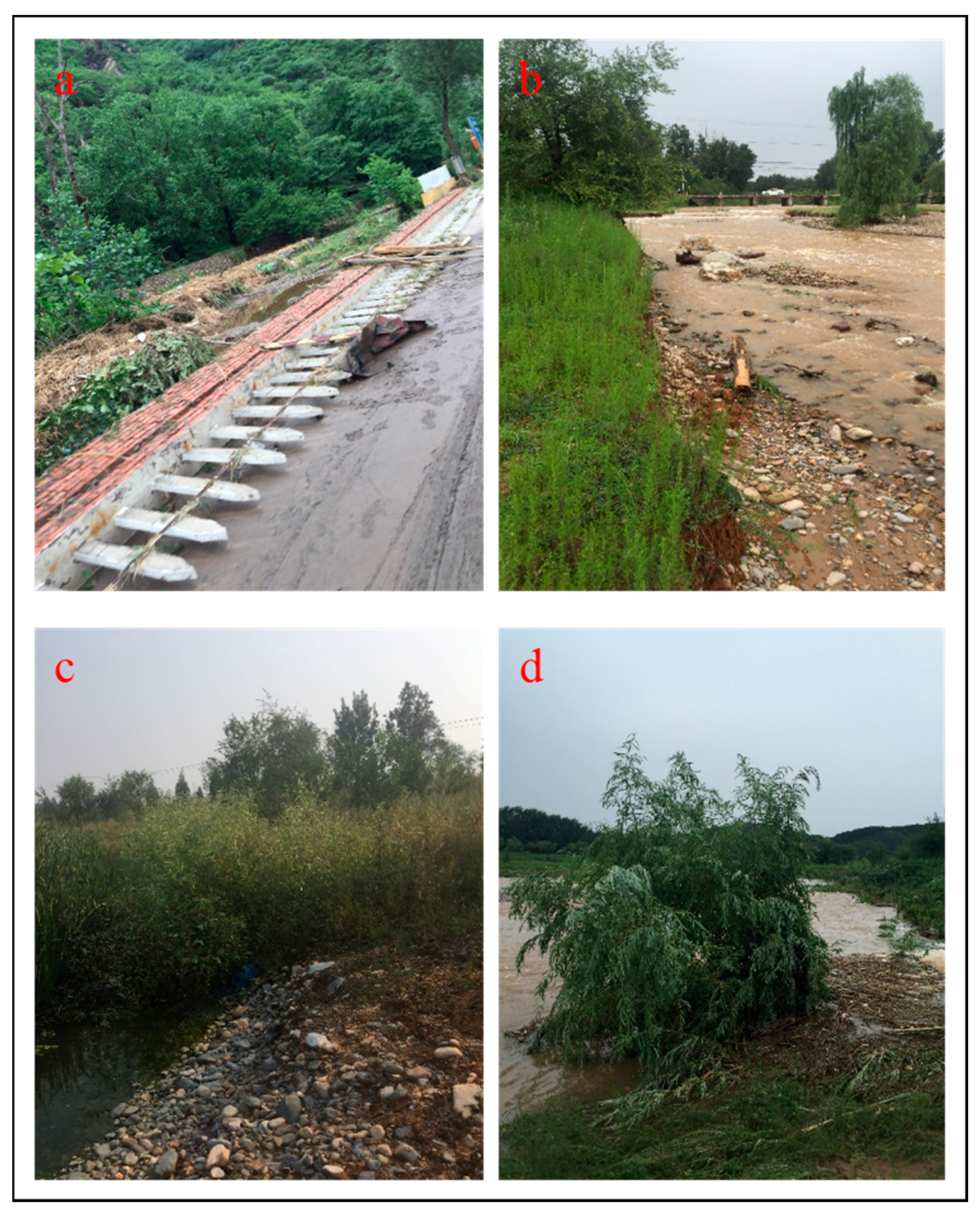
2.1. Construction Methods for Living Brush Mattress and Salix alba L. ‘Tristis’ (LBS)

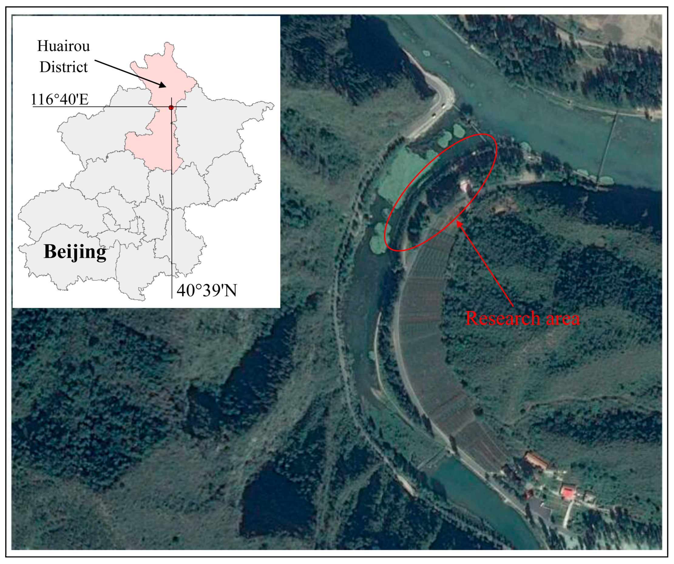
The live brush mattress comprises living shoots of plants (approximately 20 mm in diameter) that have been spread in horizontal rows on the surface of the bank such that the thick end is soaked in water and the soil is covered above the shoots. The interspaces between each living shoot are as small and uniform as possible to ensure greater bank protection benefits [40]. After construction, a number of newborn plants will grow on the living shoots. Our research is aimed at these individual newborn plants.

The structural material of LBS is Salix alba L. ‘Tristis’ living shoots with a diameter of 20 mm. The interspace between adjacent shoots is approximately 0.5 m. A schematic of the LBS structure is shown in Figure 2. The LBS was constructed before the end of the plant dormancy period in 2009, 2010, 2011, 2012, 2015 and 2016, with planting areas of approximately 300 m², 300 m², 180 m², 180 m², 300 m² and 300 m², respectively. In the first year after construction, a large number of herbs were found growing in the interspaces between the living shoots, and weeding and watering were undertaken twice a month for the first three months. In the following year after construction, few herbs were found, and only a weeding operation was undertaken in May. After five years of growth, few plants were growing in the interspaces, and the LBS had colonized.

2.2. Site Details

The experiment was conducted at a bank along the Liuli River in the Huairou District, Beijing, China (alt.: 243 m, lat.: 40°39′ N, long.: 116°40′ E) (Figure 3). Following artificial transformation in accordance with the original riverbank terrain, the soil distribution 0–0.4 m below the surface at the experiment site is sandy loam (measured by the hydrometer method) with small gravel, and below 0.4 m, loamy sand (measured by the hydrometer method) with gravel is found. After land preparation, the riverbank slope was transformed to be consistently 15°.

2.3. Tree Selection and Extraction

Twenty-four LBS trees, eight each of 1-year-old, 5-year-old and 7-year-old trees, were chosen for the experiment. Five trees were used for the morphological study, and three trees were used for shear strength tests of each age. Before sample collection, the basic condition of the LBS in the plot was investigated. The results are shown in

Table 1. Basic conditions of various growth years.

Age	1			5			7
Plot Area (m2)	3 m × 2 m			3 m × 4 m			3 m × 4 m
Plot Number	1	2	3	1	2	3	1	2	3
Plot Slope	15°	15°	15°	15°	15°	15°	15°	15°	15°
Number of Trees	8	8	8	13	9	11	12	7	8
Mean Basal Diameter (mm)	10.7	10.2	10.6	75.4	82.7	86.8	115.6	130.4	113.2

. According to the arithmetic mean of the basis diameter of the survey, a well-grown single tree that had no neighbors [20] within a radius of nearly 1 m was regarded as the standard wood.

The root system exposure method, which requires a heavy workload but can provide more comprehensive root information, was used in this study. Excavation was conducted from 15 August to 17 September 2016, and from 3 August to 25 August 2017. Before excavation, each tree was cut horizontally at the point immediately above where the top-most root emerged from the stem, and the aspect was marked using a permanent pen. A trench with the stem at the center was dug by hand, trowel and water rinsing until all roots were exposed. After excavation, efforts were made to ensure that the root system remained unchanged, and the sample was transported to the laboratory for digitizing. Inevitably, roots were broken during excavation, and these broken roots were collected, marked, and reconstructed in the laboratory.

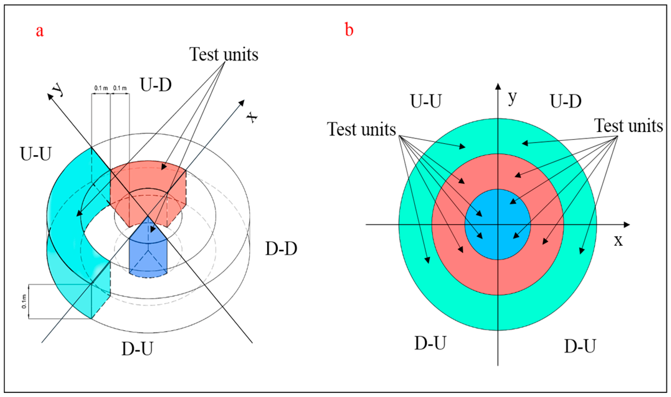
2.4. Root System Parameter Measurements

Four test zones were established for each sample, divided into the upslope-upstream face (hereafter referred to as U-U), the downslope-upstream face (hereafter referred to as D-U), the upslope-downstream face (hereafter referred to as U-D) and the downslope-downstream face (hereafter referred to as D-D). In each test zone, the space was divided into many test units composed of various special geometric shapes. In the vertical direction, the thickness of the geometric shape was 0.1 m, and in the horizontal direction, demi-semi-circles or annuluses were divided with individual radii of 0.1 m (Figure 4).

The maximum vertical depth (MVD) from the surface, the maximum lateral distance (MLD), and the diameter of every root in each test unit from the stem were measured. The root biomass values were recorded after oven-drying at 70 °C for 48 h [41]. The number of roots and the root cross-sectional area were recorded during shear strength tests, and the content was converted into unit volume.

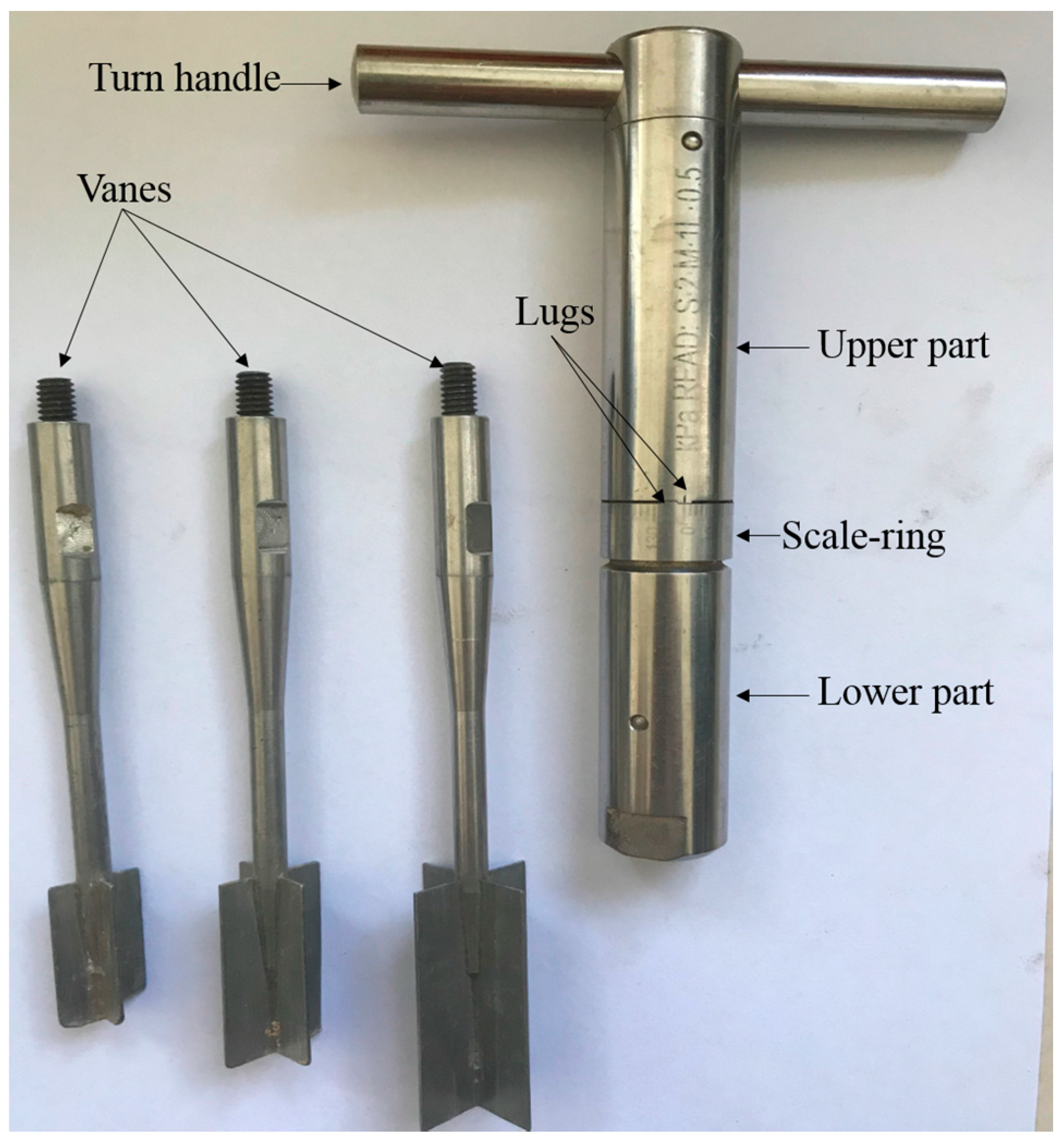
2.5. Shear Strength Determination

The shear strength was measured using a field inspection vane tester (Figure 5), which was used to measure the in situ undrained shear strength of the soil [13]. The lower and upper parts of the instrument are connected by a threaded joint. The scale-ring is also supplied with threads and follows the upper part of the instruments by means of two lugs. The 0-point is indicated by a line on the upper part. When the handle is turned, the spring deforms, and a mutual angular displacement formed between the upper and lower parts of the instrument, with the scale-ring following the upper part of the instrument. When failure is obtained, the scale-ring will remain in its position due to the friction in the threads. The size of the displacement depends on the torque that is necessary to turn the vane. The product of the scale reading and the vane coefficient is the measured value of the soil shear strength. The measuring range of the instrument is from 0 to 260 kPa when three differently sized vanes (16 × 32, 20 × 40 and 25.4 × 50.8 mm) are used, and the corresponding vane coefficients for each size are 2, 1 and 0.5, respectively. The measurement accuracy is within 10% of the reading.

Profile quantities parallel to the bank slope were excavated, and the shear strength was recorded for each unit (similar to Section 2.4). Certain outliers (e.g., samples with no obvious signs of root rupture or samples for which boulders were encountered during the test) were eliminated. Although it cannot be denied that the soil shear strength test method used in this study has some shortcomings for soils permeated by large roots, the sample plot was on the riverbank, and the soil contained large amounts of gravel of an uneven distribution, which can greatly affect the measurements obtained with other methods such as the shear box test [18,42]. We attempted to increase the number of tests in each unit as much as possible to compensate for the defects caused by the methods used in this study.

During the test, at greater distances from the stem, no roots were found in a number of test units. The shear strength of these units was considered to be the shear strength of the pure soil. For each root-soil composite unit, the shear strength enhancement value was determined by a subtraction operation of the shear strength between this unit and the pure soil.

The fact that coarse roots tend to act as separate anchors rather than as a component reinforcing soil strength has been confirmed in past studies [43]. Compared with fine roots, coarse roots make no significant contribution to improving the shear strength of root-soil composites [44]. In this study, the relationships between the number and cross-sectional area of fine roots and the soil shear strength were revealed. In addition to hair roots, the diameter of the fine root was defined as less than 5 mm [45].

2.6. Statistical Analysis

The data were analyzed using the statistics package SPSS 18.0 (SPSS Inc., Chicago, IL, USA). Multiple comparisons of the tree height, stem diameter, root biomass, maximum lateral root extent, and maximum root depth were performed using Tukey’s honestly significant difference test for the three tree ages. Analysis of variance (ANOVA) was performed to test the effect of age on root biomass in different slope positions (upslope and downslope) and a paired t-test was performed to test the effect of slope position on root biomass for each age. Regression analyses were performed to investigate the relationships between the root biomass and depth, between the root biomass and the distance from the stem, between the shear strength and the number of roots, and between the shear strength and cross-sectional area.

3. Results

3.1. LBS Dimensions

Table 2. General measurements of the excavated Salix alba L. ‘Tristis’ (LBS).

Age (Year)	N	H (m)	D (mm)	RB (g)	MLD (m)	MVD (m)
1	5	2.01 ± 0.35 a	9.16 ± 1.36 a	24.5 ± 7.02 a	0.45 ± 0.06 a	0.20 ± 0.03 a
5	5	9.79 ± 1.00 b	79.92 ± 11.46 b	507.28 ± 49.00 b	1.00 ± 0.20 b	1.46 ± 0.11 b
7	5	14.11 ± 1.22 c	122.08 ± 11.66 c	1006.25 ± 157.85 c	1.27 ± 0.11 c	1.73 ± 0.07 c

Note: Data are represented as means and standard deviations (mean ± SD). N = sample size; H = tree height; D = stem diameter at ground level; RB = root biomass; MLD = maximum lateral root extent; MVD = maximum root depth. Different letters in the same column indicate a significant difference at α = 0.05.

shows selected basic parameters of the excavated samples. The basal diameters of all trees were close to the average of the plot.

After 5 and 7 years of growth, the root biomass was 20 and 41 times the biomass of the 1-year-old LBS, respectively. As observed during the extraction process, the LBS had a large number of adventitious roots, and the main root was not formed in the early stage of planting. After 5 and 7 years of growth, the main root was formed and extended to above 1.46 m and 1.73 m, respectively. In terms of the basic parameters over time, both the tree height and the basal diameter increased steadily. The MLD development was relatively fast in the first 5 years and then became slower in the next two years, in contrast with the development of the MVD.

The approximate relationships between the tree height (H) and the MLD and MVD are presented in

Table 3. Relationships between the tree height (H) and the maximum lateral distance (MLD) and maximum vertical depth (MVD) of the root system.

Age (Year)	MLD/H	MVD/H
1	0.22	0.1
5	0.1	0.15
7	0.09	0.12

. Note that with the exception of the MLD, that was measured for the 1-year-old LBS, both the MVD and MLD are approximately 10% of the tree height.

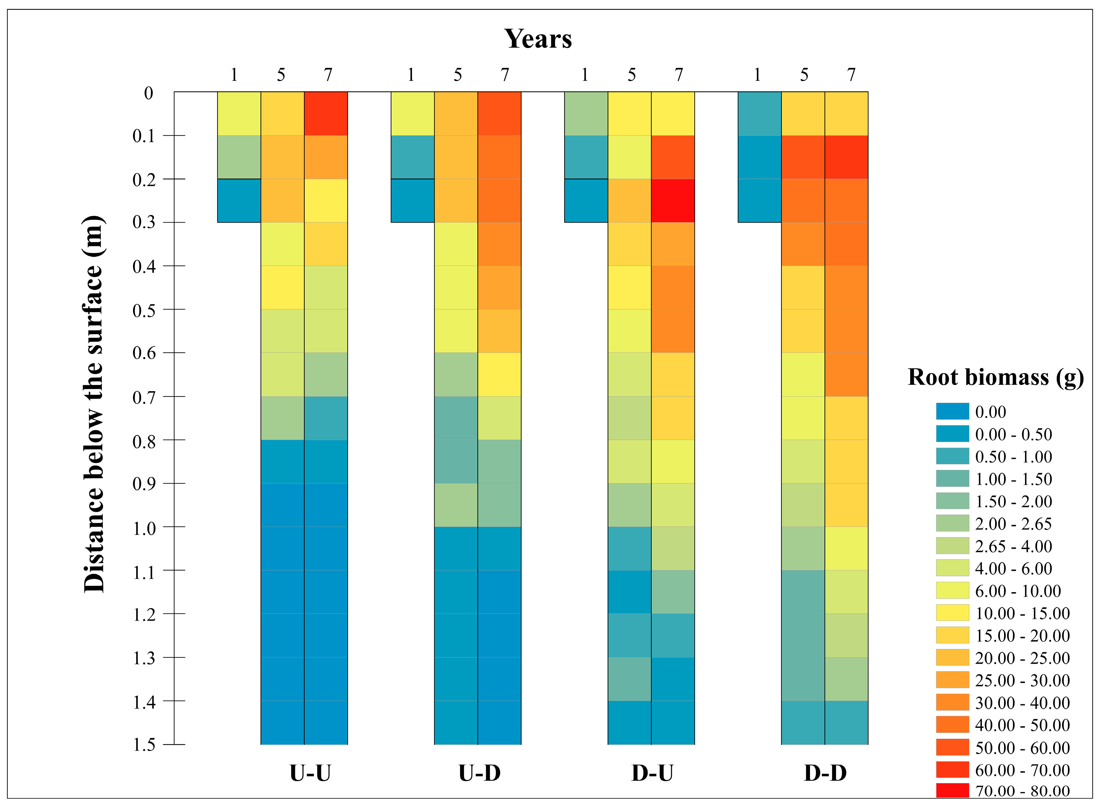
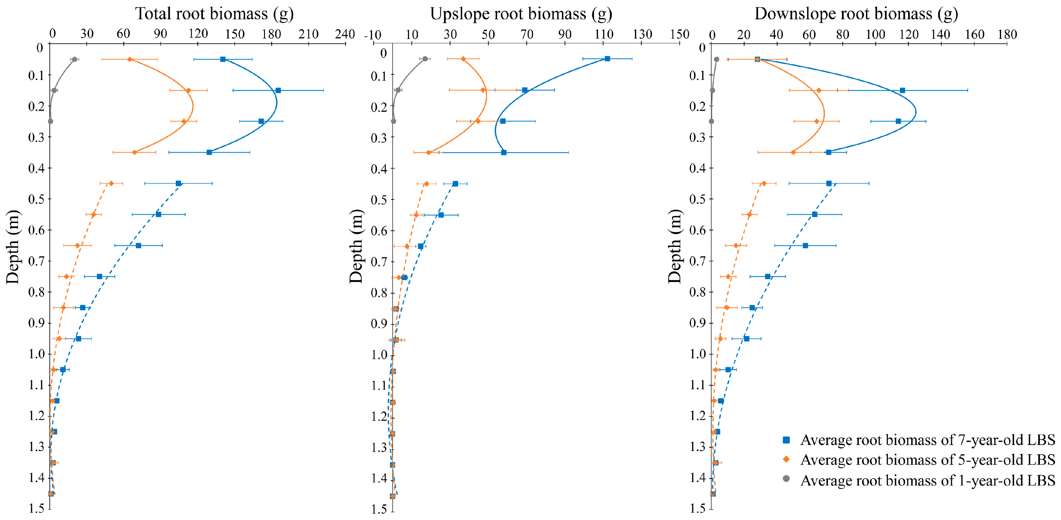
3.2. Spatio-Temporal Root Biomass Distribution with the Depth below the Ground Surface

The spatio-temporal root biomass distribution is shown in Figure 6. The root biomass was less on the upslope face than on the downslope face, and the biomass was larger on the downstream face than on the upstream face, except in the 1-year-old LBS. As observed during the excavation, the roots of the LBS developed on both sides of the living shoot buried in the soil. Therefore, the root growth symmetry of the LBS was determined from the biomass on both sides of the living shoot (namely the upstream and the downstream faces of the slope, respectively). When the colors of the color blocks in the figure (representing the root biomass content of each test unit) at the same slope position are compared, similar colors are observed on the upstream and downstream faces for the 1-year-old LBS, indicating that the root system showed obvious symmetry in these two zones. After 5 years of growth, this symmetry was preserved only in the soil above 0.4 m in the upslope area. After the 7th year, this symmetry was no longer detectable.

In general, roots located in the upslope zone were concentrated primarily in the 0–0.4 m soil layer or in the 0.1–0.7 m downslope layer. In the 0–0.1 m soil layer, the root biomass was much larger in the upslope zone than in the downslope zone; however, at an increased depth, the result was the opposite. The root biomass distributed in the downslope zone was deeper than that in the upslope zone, except for the 1-year-old LBS. For example, for the 5-year-old LBS, color blocks representing less than 10 g of biomass are found below 0.5 m in the U-U zone and 0.3 m in the U-D zone, while for the downslope zone, such color blocks are found below 0.5 m in the D-U zone and 0.6 m in the D-D zone. The LBS root system exhibited characteristics upslope growth, meaning that the root system in the upslope zone grew close to the surface, whereas the growth behavior in the downslope zone was the opposite.

The root biomass distributions with depth in the upslope and downslope zones were analyzed (Figure 7). The root biomasses of the 5- and 7-year-old LBS, with approximately 71% and 63% of the total residing in the depth range of 0–0.4 m, first increased with depth and then decreased while exhibiting larger fluctuations. Therefore, this soil layer could be identified as the active layer of root growth. When the depth reached below 0.4 m, the root biomass, accounting for approximately 29% and 37% of the total, showed a steady decrease. Thus, this area could be defined as the stable layer of root growth [17]. Since the root system of the 1-year-old LBS was concentrated in the 0–0.3 m soil layer, the stable layer and the active layer could not be separately identified. The change in root biomass with depth was described by regression analysis. The optimal curve fit was identified by evaluating linear, power, logarithmic, exponential and polynomial equations in terms of their R² values.

Based on the fitting results, the relationships are best represented by the 2nd-order polynomial equation (

Table 4. Regression equations and R² values of the root material by biomass with depth in the axial direction.

		1-Year-Old	5-Year-Old	7-Year-Old
Active Layer	Total	B = 727.9d2 − 311.9d + 34.03 R2 = 0.9148	B = −2193.2d2 + 885.03d + 26.90 R2 = 0.6731	B = −2174.9d2 + 823.17d + 106.31 R2 = 0.4272
	Upslope	B = 623.2d2 − 265.68d + 28.68 R2 = 0.921	B = −902.55d2 + 304.34d + 23.41 R2 = 0.5164	B = 1091.8d2 − 610.72d + 139.09 R2 = 0.5717
	Downslope	B = 104.7d2 − 46.22d + 5.35 R2 = 0.711	B = −1290.6d2 + 580.69d + 3.50 R2 = 0.4486	B = −3266.7d2 + 1433.9d − 32.78 R2 = 0.7217
Stable Layer	Total		B = 77.72d2 − 190.25d + 116.66 R2 = 0.8665	B = 140.34d2 − 371.09d + 246.37 R2 = 0.8891
	Upslope		B = 32.01d2 − 75.92d + 44.20 R2 = 0.7618	B = 64.561d2 − 152.06d + 87.29 R2 = 0.8966
	Downslope		B = 47.71d2 − 114.33d + 72.47 R2 = 0.8418	B = 75.78d2 − 219.03d + 159.08 R2 = 0.8368

Note: B = root biomass (g); d = distance below the surface (m).

). From these equations, it is possible to estimate the root biomass at any depth under similar site conditions.

The growth rates of the total root biomass from 1 to 5 years and from 5 to 7 years in the vertical direction are shown in

Table 5. The growth rate of total root biomass in each soil layer in the vertical direction.

Vertical Depth (m)	Growth Rate
	1−5 Years	5−7 Years
0.0–0.1	11.16	37.79
0.1–0.2	27.44	36.42
0.2–0.3	27.05	31.38
0.3–0.4	17.19	30.38
0.4–0.5	12.50	27.23
0.5–0.6	8.92	26.31
0.6–0.7	5.64	24.75
0.7–0.8	3.40	13.48
0.8–0.9	2.77	7.86
0.9–1.0	1.98	7.74
1.0–1.1	0.80	3.74
1.1–1.2	0.57	1.80
1.2–1.3	0.56	0.85
1.3–1.4	0.71	−0.08
1.4–1.5	0.22	0.13

. The growth rates in the first four years were significantly smaller than those from 5 to 7 years in the soil layers 0–1 m below the surface. In the 1–1.3 m layers, the growth rates from 5 to 7 years were still greater than those from 1 to 5 years, but the growth trend was gradual. When the soil depth reached 1.3 m or more, the growth rates from 5 to 7 years were no longer greater than those from 1 to 5 years.

The paired t-test was performed to test the effect of slope position (upslope and downslope) on root biomass for each age and the ANOVA was performed to test the effect of age on root biomass in different slope positions (

Table 6. Results of paired t-test and analysis of variance (ANOVA) for evaluating the effects of slope position and age on the root biomass across different ranges of soil depth.

p-Value
Soil Depth (m)	Paired t-Test			ANOVA
	Slope Position			Age
	1-Year-Old	5-Year-Old	7-Year-Old	Upslope	Downslope
0.0–0.1	<0.01	0.308	<0.01	<0.01	0.030
0.1–0.2	0.038	0.271	0.090	<0.01	<0.01
0.2–0.3	0.398	0.130	0.012	<0.01	<0.01
0.3–0.4	-	0.062	0.477	<0.01	<0.01
0.4–0.5	-	0.019	0.018	<0.01	<0.01
0.5–0.6	-	<0.01	<0.01	<0.01	<0.01
0.6–0.7	-	0.060	<0.01	<0.01	<0.01
0.7–0.8	-	0.045	<0.01	<0.01	<0.01
0.8–0.9	-	0.020	<0.01	0.061	<0.01
0.9–1.0	-	0.227	<0.01	0.428	<0.01
1.0–1.1	-	0.037	0.011	0.471	<0.01
1.1–1.2	-	0.122	<0.01	0.397	<0.01
1.2–1.3	-	0.035	<0.01	0.397	<0.01
1.3–1.4	-	0.160	0.021	0.397	0.142
1.4–1.5	-	0.174	0.012	0.397	0.078

Note: The boldface values indicate significant differences (p < 0.05). The symbol “-” indicates that there was no root in this soil layer.

). Considering the effect of slope position on the root biomass, in the 1st year, the slope position influenced the root biomass at the soil depths of 0–0.2 m, and in the 5th year, impacted the root biomass at the depths of 0.4–0.6 m, 0.7–0.9 m, 1.0–1.1 m and 1.2–1.3 m. In the 7th year, the slope position affected the root biomass throughout the whole system except at the depths of 0.1–0.2 m and 0.3–0.4 m. Considering the effect of age on the root biomass, in the upslope area, the age influenced the root biomass at the soil depths of 0–0.8 m, and in the downslope area, it impacted the root biomass at the depths of 0–1.3 m.

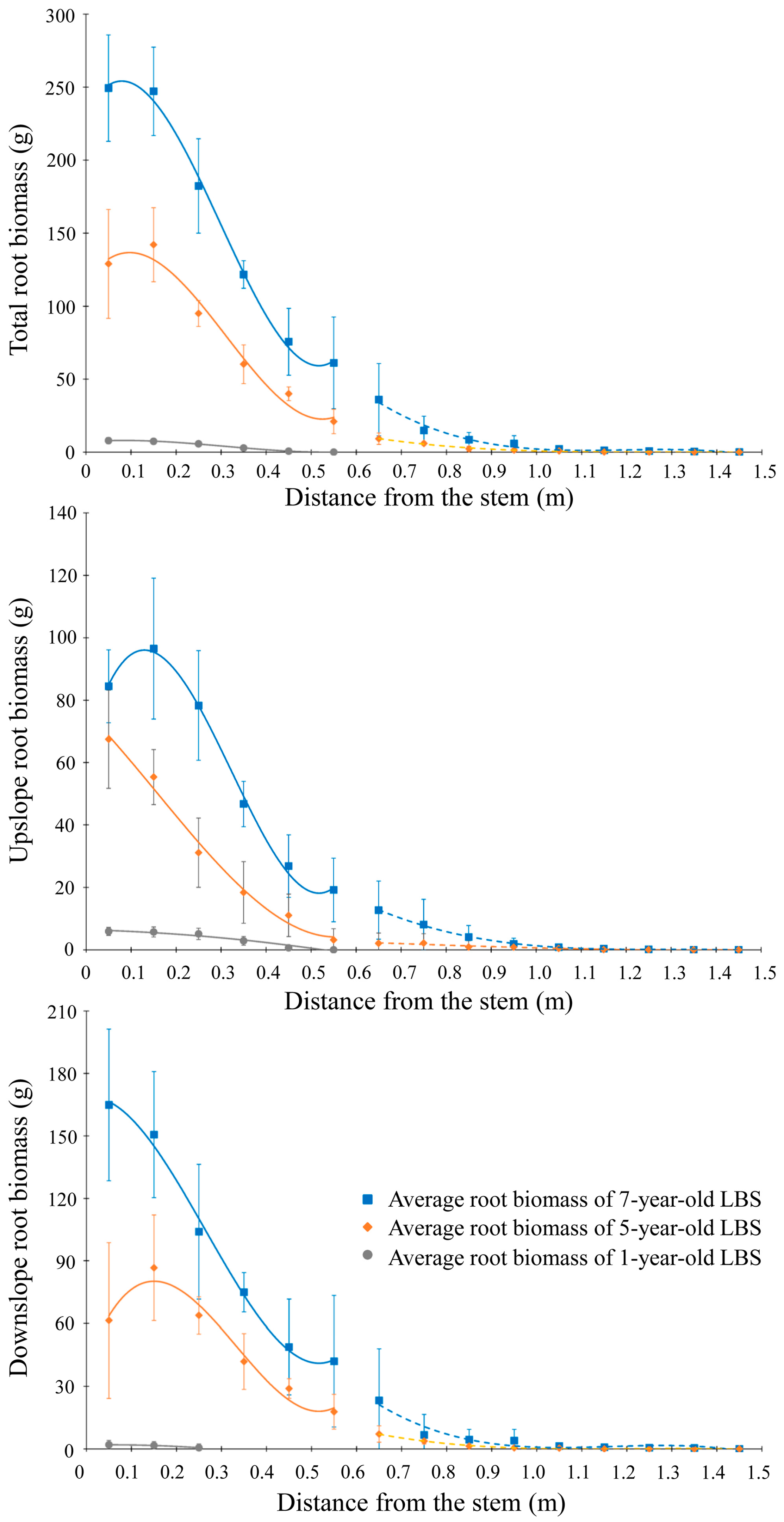
3.3. Spatio-Temporal Root Biomass Distribution with Lateral Distance from the Tree Stem

The root biomass distributions with lateral distance from the tree stem were analyzed (Figure 8). The root biomasses of the 5- and 7-year-old LBS, with approximately 93% and 96% of the total residing in the distance range of 0–0.6 m, first increased with distance and then decreased while exhibiting larger fluctuations. Therefore, this soil layer could be identified as the active layer of root growth. When the distance reached 0.6 m, the root biomass, accounting for approximately 7% and 4% of the total, showed a steady decrease. Thus, this area could be defined as a stable layer of root growth. For the 1-year-old LBS, the roots were distributed entirely within 0–0.6 m of the lateral distance. The root biomass in the downslope was slightly larger than that in the upslope area, and approximately 80% of the root materials were concentrated in the 0–0.4 m lateral distance. Contrary to expectations [17], the root biomass variation with the horizontal distance in certain growth periods did not show a decreasing trend at the beginning but decreased after the first increase in the 0.1–0.2 m soil layer. The variation of root biomass and the horizontal distance from the tree stem were fitted using regression analysis (

Table 7. Regression equations and R² values for the variation of the root biomass with the distance from the stem in the horizontal direction.

		1-Year-Old	5-Year-Old	7-Year-Old
Active layer	Total	B = −5.2l2 − 14.70l + 9.11 R2 = 0.8109	B = 2909.4l3 − 2713.2l2 + 443.9l + 116.4 R2 = 0.8426	B = 4651.7l3 − 4162l2 + 573.2l + 232.5 R2 = 0.895
	Upslope	B = −15.80l2 − 3.94l +6.44 R2 = 0.7758	B = 368.7l3 − 173.1l2 − 147.8l + 76.4 R2 = 0.8612	B = 2666.1l3 − 2587.3l2 + 535.9l + 64.2 R2 = 0.8406
	Downslope	B = -35.7l2 + 3.72l + 1.89 R2 = 0.3868	B = 2540.6l3 − 2540.1l2 + 591.7l + 40 R2 = 0.6702	B = 1985.6l3 − 1574.7l2 +37.2l + 168.3 R2 = 0.8358
Stable layer	Total		B = −38.6l3 + 147.2l2 − 187.1l + 79.3 R2 = 0.8225	B = −218.8l3 + 783.6l2 − 930.7l + 368 R2 = 0.6232
	Upslope		B = 3.9l3 − 7.93l2 + 0.4l + 4.3 R2 = 0.2126	B = −48.1l3 + 186.3l2 − 240.7l + 103.9 R2 = 0.5382
	Downslope		B = −42.5l3 + 155.2l2 − 187.5l + 75.1 R2 = 0.5966	B = −170.7l3 + 597.3l2 − 689.9l + 264.2 R2 = 0.6001

Note: B = root biomass (g); l = lateral distance from the tree stem (m).

). The results showed that the root biomass of 1-year-old LBS was best fitted by the 2rd-order polynomial equation, and that of the 5- and 7-year-old LBS by the 3rd-order polynomial equation.

Similar to the presentation of the results in Section 3.2, the growth rates of the total root biomass from 1 to 5 years and from 5 to 7 years in the horizontal direction are shown in

Table 8. The growth rate of the total root biomass in each soil layer in the horizontal direction.

Distance from the Stem (m)	Growth Rate
	1−5 Years	5−7 Years
0.0–0.1	30.26	60.19
0.1–0.2	33.67	52.53
0.2–0.3	22.32	43.65
0.3–0.4	14.33	30.71
0.4–0.5	9.83	17.81
0.5–0.6	5.26	20.05
0.6–0.7	2.30	13.36
0.7–0.8	1.48	4.43
0.8–0.9	0.58	3.11
0.9–1.0	0.36	2.22
1.0–1.1	0.21	0.69
1.1–1.2	0.03	0.56
1.2–1.3	0.01	0.37
1.3–1.4	0.01	0.21

.

The growth rates of the root biomass in the first four years were smaller than that in the 5–7 years in the 0–0.7 m soil layer from the stem. In the 1–1.4 m layer, the growth rates over 5 to 7 years were still greater than that over 1 to 5 years, but the growth trend was gradual.

The paired t-test was performed to test the effect of slope positions (upslope and downslope) on root biomass for each age and the ANOVA was performed to test the effects of age on root biomass in different slope position (

Table 9. Results of paired t-test and ANOVA for evaluating the effects of slope position and age on the root biomass across different distances from the stem.

Distance from the Stem (m)	Paired t-Test			ANOVA
	Slope Position			Age
	1-Year-Old	5-Year-Old	7-Year-Old	Upslope	Downslope
0.0–0.1	<0.01	0.376	0.012	<0.01	<0.01
0.1–0.2	<0.01	0.132	<0.01	<0.01	<0.01
0.2–0.3	<0.01	0.018	0.043	<0.01	<0.01
0.3–0.4	0.010	0.016	0.038	<0.01	<0.01
0.4–0.5	0.052	0.017	0.092	<0.01	<0.01
0.5–0.6	0.374	0.065	0.051	<0.01	<0.01
0.6–0.7	-	0.219	0.054	<0.01	<0.01
0.7–0.8	-	0.584	0.671	0.062	<0.01
0.8–0.9	-	0.755	0.857	0.049	<0.01
0.9–1.0	-	0.693	0.331	0.108	0.070
1.0–1.1	-	0.898	0.689	0.231	0.230
1.1–1.2	-	0.374	0.565	0.292	0.111
1.2–1.3	-	0.374	0.404	0.175	0.117
1.3–1.4	-	0.374	0.293	0.619	0.257
1.4–1.5	-	-	-	-	-

Note: The boldface values indicate significant differences (p < 0.05). The symbol “-” indicates that there was no root in this soil layer.

). Considering the effect of slope position on the root biomass, in the 1st year, the slope position influenced the root biomass at the lateral distances of 0–0.4 m, and in the 5th year, it impacted the root biomass at the lateral distances of 0.2–0.5 m. In the 7th year, the slope position influenced the root biomass at the lateral distances of 0–0.4 m. Considering the effect of age on the root biomass, in the upslope area, the age influenced the root biomass at the lateral distances of 0–0.7 m and 0.8–0.9 m, and in the downslope area, it impacted the root biomass at the lateral distances of 0–0.9 m.

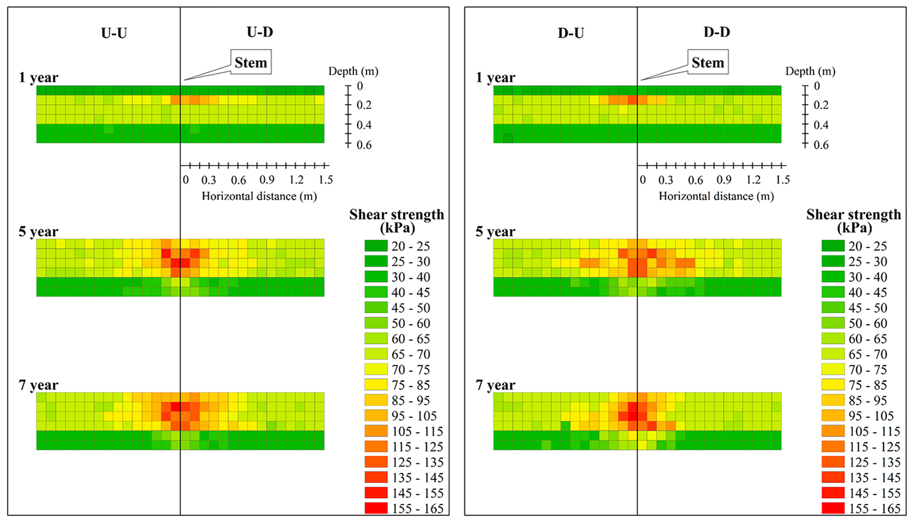
3.4. Spatio-Temporal Distribution of the Soil Shear Strength with LBS Roots

Figure 9 describes the shear strength distribution of the soil with LBS roots. Because the water level exceeded the riverbank height, it was impossible to determine the shear strength of certain deeper soil layers; thus, testing was conducted only up to 0.6 m below the surface. An unambiguous stratification of shear strength caused by the unique distribution characteristics of the riparian soil structure occurred 0.4 m underground. The maximum shear strength of the root-soil composite was approximately 159.61 kPa in the upper layer (0–0.4 m below the surface) and 80.94 kPa in the lower layer (0.4–0.6 m below the surface) (

Table 10. The shear strengths of the pure soil and the root-soil composite.

Depth (m)	SSP (kPa)	MSSC (kPa)	ESS (kPa)
0–0.4	67.61 ± 4.41	159.61	24.05 ± 22.27
0.4–0.6	36.78 ± 2.33	80.94	11.74 ± 10.53

Note: SSP and ESS data are represented as means and standard deviations (mean ± SD). SSP = shear strength of the pure soil; MSSC = maximum shear strength of the root-soil composite; ESS = average soil shear strength enhancement values of all root-soil composite units.

). In the upper and lower layers, the shear strength of pure soil was 67.61 kPa and 36.78 kPa, respectively (Table 10). The reinforcement effect of the LBS roots on the soil was mainly concentrated in the horizontal layer 0.6 m from the stem. When the distance was more than 0.6 m, the strengthening effect was not easily detectable. In the upslope zone, the distribution range of the shear strength in the horizontal direction markedly decreased with an increase in soil depth. By contrast, in the downslope zone, the distribution range of the shear strength in the horizontal direction initially increased and then markedly decreased with increasing soil depth. In general, the range of the shear strength increased with the tree age. For a given unit, however, the shear strength did not necessarily increase with age; for example, in the U-U region, the horizontal 0.1–0.2 m layer, and the vertical 0.1–0.2 m layer, the soil shear strength of the 7-year-old LBS was less than that of the 5-year-old LBS. The shear strength of the 1-year-old LBS in the 0–0.1 m soil layer varied between 20 kPa and 31 kPa, which was obviously less than the shear strength of the pure soil. In order to demonstrate that the use of LBS has an advantage over other plant species in improving soil shear strength, the average soil shear strength enhancement values of all root-soil composite units, 24.05 kPa and 11.4 kPa in the upper and lower layers, respectively, were calculated (Table 10).

The regression relationships between the shear strength enhancement and the root materials for the 5- and 7-year-old LBS are shown in Figure 10. The results show that both the number of roots and the root cross-sectional area per unit volume were highly significantly correlated with the enhancement values of the soil shear strength (p < 0.01).

4. Discussion

4.1. Spatio-Temporal Dynamic Distribution Characteristics of the LBS Root System

Among all tree ages, the MVD and MLD corresponded to a relatively small proportion of the tree height. The relationships were 0.1 H < MVD < 0.15 H and 0.09 H < MLD < 0.22 H. These ratios are obviously less than the approximate relationships of H < Dr < 2 H reported by Greenway [46], Wu [47], and Docker and Hubble [17], where Dr = the root diameter = 2MLD. These findings show that the extents of the LBS root system in the vertical and lateral slope directions were small relative to the shoot growth aboveground. Furthermore, the MLDs of the 5- and 7-year-old LBS were 1 m and 1.27 m, respectively, corresponding to only 1/8 and 1/10 of the MLD of 5- and 7-year-old Veronese poplars, respectively [19]. Therefore, the LBS had a small root system in general. Although the lateral root extension of the LBS was small, the living shoots that were used to construct the LBS limited its growth position, and the interspaces between the living shoots were also small to ensure that the LBS would form a root grid in the interspace of shoots and soil. According to the spatio-temporal dynamic distribution of the root biomass, the roots were distributed primarily in a cylindrical soil pattern with an approximate radius of 0.4 m and a thickness of 0.5 m. This characteristic arose because the root system was mainly distributed in the shallow soil layer, as reported by Mclvor et al. [19]. For the 1-year-old LBS, 95% of the total root biomass was distributed in the first 0.1 m of depth; thus, this shallow root biomass was obviously larger than the root biomass in the 0.1–0.3 m layer underground. This result indicates that in the early planting stage, the roots of the LBS were concentrated in the 0–0.1 m layer and developed primarily in the horizontal direction. Thus, the ratio between the MLD and the tree height for the 1-year-old trees is greater than that for the LBS at other ages, as shown in Table 3. The total root biomasses at the depth of 0.1–0.2 m for the 5- and 7-year-old LBS and at 0–0.1 m for the 1-year-old LBS were the largest of any soil layer (Figure 7). These findings indicate that the roots of the LBS were able to develop even in the thinner soil layer on the lower part of the slope. For original bank slope structures such as a rocky bank slope, root development would be difficult. However, an artificial soil covering could create a growing environment for the roots of LBS.

Symmetry of the 1-year-old LBS root system was found between the upstream and downstream faces. This finding is consistent with the symmetries of other plant species’ root systems during the seedling period [48,49]. However, with increasing time, the root system symmetry was no longer evident. Root growth reacts to mechanical impedances and soil nutrients [50]. During extraction, gravels were found in the deep soil, and the random distribution of gravel and soil nutrients was probably the cause of the disappearance of symmetry. An upslope growth characteristic of LBS was also found in this study; the roots in the upslope zone were closer to the surface than the roots in the downslope zone, in contrast to the growth trend reported by Mclvor et al. [19]. In fact, however, the amount of root biomass in the downslope zone was obviously higher than that in the upslope zone; thus, it should be noted that the upslope growth explains only the direction of root growth. Our results also exhibited that, except at depths below 1.3 m, the growth rate in the last two years was greater than that in the first four years. From this discrepancy in root biomass growth rate, the root development of LBS shows a non-uniform trend in time scale over the first 7 years.

Both slope position and age had an effect on the LBS root biomass (Table 6 and Table 9). In the vertical direction, the effect of the slope position on the root biomass at different ages were different, and with aging, the influence range gradually increased. In the 1st year, the effect of slope position on root biomass was significant at depths of 0–0.2 m; in the 5th year, the effect of slope position on root biomass was mainly concentrated in deeper soil layers; in the 7th year, slope position almost influenced the root biomass in all soil layers. In addition, the influence range of age on the root biomass in the downslope area was deeper than the upslope area. This difference may be due to the upslope growth characteristic of the root of LBS. In the horizontal direction, the influence of the slope position on the root biomass at different ages was mainly concentrated in the range of 0–0.5 m. This concentration may be due to the fact that the LBS roots were mainly distributed in this soil layer at these three ages. Notably, for 5-year-old LBS, no effect of slope position on root biomass was observed in the 0–0.1 m and 0.1–0.2 m soil layers. This may indicate that there were no remarkable differences in the increments of root biomass in upslope and downslope areas in these two soil layers from 1 to 5 years. On the other hand, the effects of age on the root biomass in the upslope and downslope areas were found in the 0–0.9 m soil layers. This result may indicate that although the root biomass increases with age, in the horizontal direction, the LBS roots frequently grew only in the soil layers at 0–0.9 m.

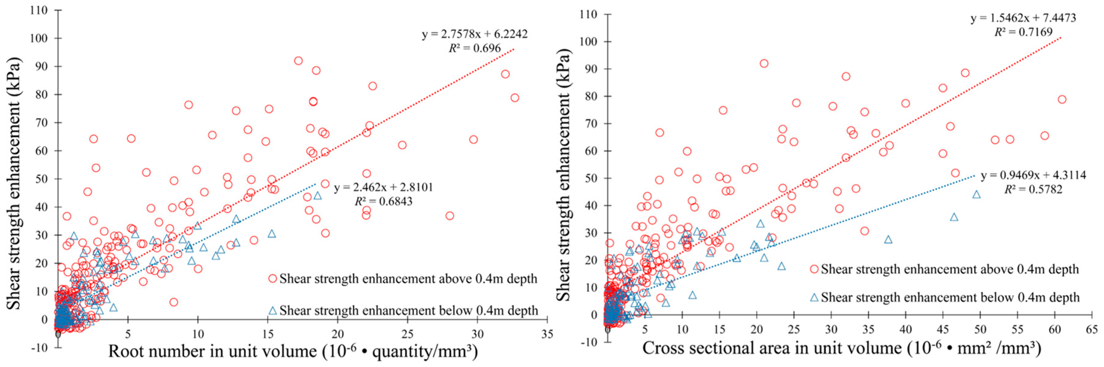
4.2. Soil Shear Strength Enhancement by the LBS Root System

From the distribution of the soil shear strength (Figure 9), it was found that the shear strength enhancement was distributed in the soil with a conical shape, and with an increase in the lateral distance, the enhancement became no longer obvious; this result is consistent with the conclusion offered by Fan and Lai [14] and indicates that plant roots provide a cone-shaped soil shear strength enhancement zone in the soil below that is centered on the stem [17,44,51]. In the first five years, the plant age has an obvious influence on the range of the root-induced enhancement of the soil shear strength. With aging, the soil shear strength gradually expands in both the horizontal and vertical directions. However, the effect of age on the soil shear strength expansion was not obvious between the 5th and 7th years. Furthermore, in some soil layers closer to the stem, the shear strength did not increase but rather decreased. This result may demonstrate that the contribution of plants to riverbank stability cannot be determined solely from the growth period of the plants but mainly from the root distribution, which has also been demonstrated by previous studies [17]. In the 1-year growth stage after construction, the backfill was loose, and a large number of adventitious roots were growing in the first 0.1 m depth layer. Most of the roots were pulled out of the soil rather than shearing during the test. This effect caused the soil shear strength provided by the 1-year-old LBS root system in the 0–0.1 m depth layer to be less than that of other units.

The significant linear relationship between the shear strength enhancement by roots in the diameter class from 0 to 5 mm and the number of roots or the root cross-sectional area was similar to that reported in earlier studies [43,52]. These results demonstrate that fine roots mainly increase soil shear strength, while thicker roots anchor the soil in the vertical direction [21,44]. The number of roots in the 0–5 mm diameter class decreased with vegetation development in some soil layers close to the stem. This effect may explain why the shear strength did not increase but decreased.

The maximum enhancement values in the upper and lower layers were approximately 1.3 and 1.2 times with respect to the pure soil (calculated from Table 10). This finding indicates that the LBS roots had an obvious strengthening effect on the soil. The average soil shear strength enhancement values of LBS (Table 10) were 24.05 kPa and 11.4 kPa in the upper and lower soil layers, respectively. Compared with the living brush mattress constructed using Salix babylonica L. [5], the enhancement value of LBS is larger. Liu et al. used the pull-out test to compare the capability of Populus canadensis Moench, Amorpha fruticosa L., and LBS, which are dominant plant species suitable for soil bioengineering technology, to reinforce soil. The capabilities of Populus canadensis Moench and LBS were similar [37]. However, the vertical distribution of the Populus canadensis Moench root system [39] was smaller than that of LBS. This caused enhanced range of soil shear strength for Populus canadensis Moench that was less than that of LBS. Although the capability of individual Amorpha fruticosa L. was the largest [37], the survival rate of planting is much lower than that of LBS using soil bioengineering technology [38]. Therefore, it is not guaranteed that Amorpha fruticosa L. can form a dense population on the slope to improve the stability of the riverbank. Moreover, Guo [53] measured the tensile strength of the LBS roots using tensile tests. Compared with Picea abies (L.) H. Karst. and Ostrya carpinifolia Scop. [54], the roots of LBS had greater tensile strength. Based on the Wu’s model theory [29,47], this finding indirectly indicated that the contribution of LBS roots to enhance soil shear strength is greater than the contributions of Picea abies (L.) H. Karst. and Ostrya carpinifolia Scop. Based on these results, we speculate that LBS has a higher efficiency for soil protection, which further confirms the advantages of LBS for riverbank restoration engineering.

In this study, we investigated the root distribution characteristics of LBS and its bank protection capacity. However, considering the results may be affected by site-specific factors, such as river morphology, river flow, riverbank structure, etc., further investigations should be conducted to test the generalization of this measure. Despite this limitation, our results suggest that LBS plays an important role in riverbank protection and represents an efficient and easily applicable engineering measure for riverbank protection.

5. Conclusions

In this study, we revealed the root distribution characteristics and bank protection capacity of LBS by investigating the root biomass and soil shear strength. Our results show that the roots of LBS exhibited characteristics of symmetry and upslope growth and were mainly distributed in a cylindrical region of the soil. Moreover, the LBS provided a conically shaped shear strength enhancement zone in the soil by means of the root system. The amount of fine roots (the number and cross sectional areas here) per unit volume significantly affected the soil shear strength enhancement value. On the basis of these results, LBS protected the riverbank via improving the soil shear strength by fine roots. Compared with other plant species, LBS showed advantages in improving the soil shear strength. Although this is a case study, our results indicate that LBS is an efficient and feasible engineering measure in the field of riverbank protection.

References

1. Cheng, X.; Chen, L.; Sun, R.; Kong, P. Land use changes and socio-economic development strongly deteriorate river ecosystem health in one of the largest basins in China. Sci. Total Environ. 2018, 616–617, 376–385. [Google Scholar] [CrossRef] [PubMed]
2. Samadi, A.; Amiri-Tokaldany, E.; Darby, S.E. Identifying the effects of parameter uncertainty on the reliability of riverbank stability modelling. Geomorphology 2009, 106, 219–230. [Google Scholar] [CrossRef]
3. Darby, S.E.; Thorne, C.R. Prediction of tension crack location and riverbank erosion hazards along destabilized channels. Earth Surf. Process. Landf. 1994, 19, 233–245. [Google Scholar] [CrossRef]
4. Yao, S.; Yue, H.; Li, L. Analysis on Current Situation and Development Trend of Ecological Revetment Works in Middle and Lower Reaches of Yangtze River. Procedia Eng. 2012, 28, 307–313. [Google Scholar] [CrossRef]
5. Li, X.; Zhang, L.; Zhang, Z. Soil bioengineering and the ecological restoration of riverbanks at the airport Town, Shanghai, China. Ecol. Eng. 2006, 26, 304–314. [Google Scholar] [CrossRef]
6. Li, M.H.; Eddleman, K.E. Biotechnical engineering as an alternative to traditional engineering methods: A biotechnical streambank stabilization design approach. Landsc. Urban Plan. 2002, 60, 225–242. [Google Scholar] [CrossRef]
7. Wang, P.; Chen, G.Q. Contaminant transport in wetland flows with bulk degradation and bed absorption. J. Hydrol. 2017, 552, 674–683. [Google Scholar] [CrossRef]
8. Bischetti, G.B.; Chiaradia, E.A.; D’Agostino, V.; Simonato, T. Quantifying the effect of brush layering on slope stability. Ecol. Eng. 2010, 36, 258–264. [Google Scholar] [CrossRef]
9. Dhital, Y.P.; Tang, Q. Soil bioengineering application for flood hazard minimization in the foothills of siwaliks, Nepal. Ecol. Eng. 2015, 74, 458–462. [Google Scholar] [CrossRef]
10. Fernandes, J.P.; Guiomar, N. Simulating the stabilization effect of soil bioengineering interventions in Mediterranean environments using limit equilibrium stability models and combinations of plant species. Ecol. Eng. 2016, 88, 122–142. [Google Scholar] [CrossRef]
11. Rauch, H.P.; Sutili, F.; Hörbinger, S. Installation of a riparian forest by means of soil bio engineering techniques—Monitoring results from a river restoration work in southern Brazil. Open J. For. 2014, 4, 161–169. [Google Scholar] [CrossRef]
12. Capilleri, P.P.; Motta, E.; Raciti, E. Experimental study on native plant root tensile strength for slope stabilization. Procedia Eng. 2016, 158, 116–121. [Google Scholar] [CrossRef]
13. Li, Y.; Wang, Y.; Ma, C.; Zhang, H.; Wang, Y.; Song, S.; Zhu, J. Influence of the spatial layout of plant roots on slope stability. Ecol. Eng. 2016, 91, 477–486. [Google Scholar] [CrossRef]
14. Fan, C.C.; Lai, Y.F. Influence of the spatial layout of vegetation on the stability of slopes. Plant Soil 2014, 377, 83–95. [Google Scholar] [CrossRef]
15. Stokes, A.; Atger, C.; Bengough, A.G.; Fourcaud, T.; Sidle, R.C. Desirable plant root traits for protecting natural and engineered slopes against landslides. Plant Soil 2009, 324, 1–30. [Google Scholar] [CrossRef]
16. Giadrossich, F.; Cohen, D.; Schwarz, M.; Seddaiu, G.; Contran, N.; Lubino, M.; Valdes-Rodriguez, O.A.; Niedda, M. Modeling bio-engineering traits of Jatropha curcas L. Ecol. Eng. 2016, 89, 40–48. [Google Scholar] [CrossRef]
17. Docker, B.B.; Hubble, T.C.T. Modelling the distribution of enhanced soil shear strength beneath riparian trees of south-eastern Australia. Ecol. Eng. 2009, 35, 921–934. [Google Scholar] [CrossRef]
18. Fan, C.C.; Tsai, M.H. Spatial distribution of plant root forces in root-permeated soils subject to shear. Soil Tillage Res. 2016, 156, 1–15. [Google Scholar] [CrossRef]
19. McIvor, I.R.; Douglas, G.B.; Hurst, S.E.; Hussain, Z.; Foote, A.G. Structural root growth of young Veronese poplars on erodible slopes in the southern north island, New Zealand. Agrofor. Syst. 2008, 72, 75–86. [Google Scholar] [CrossRef]
20. Di, I.A.; Lasserre, B.; Scippa, G.S.; Chiatante, D. Root system architecture of Quercus pubescens trees growing on different sloping conditions. Ann. Bot. 2005, 95, 351–361. [Google Scholar] [CrossRef]
21. Nicoll, B.C.; Berthier, S.; Achim, A.; Gouskou, K.; Danjon, F.; Beek, L.P.H.V. The architecture of Picea sitchensis, structural root systems on horizontal and sloping terrain. Trees 2006, 20, 701–712. [Google Scholar] [CrossRef]
22. Yang, X.; Blagodatsky, S.; Liu, F.; Beckschäfer, P.; Xu, J.; Cadisch, G. Rubber tree allometry, biomass partitioning and carbon stocks in mountainous landscapes of sub-tropical China. For. Ecol. Manag. 2017, 404, 84–99. [Google Scholar] [CrossRef]
23. Luo, T.; Luo, J.; Pan, Y. Leaf traits and associated ecosystem characteristics across subtropical and timberline forests in the Gongga Mountains, Eastern Tibetan Plateau. Oecologia 2005, 142, 261–273. [Google Scholar] [CrossRef] [PubMed]
24. Czernin, A.; Phillips, C. Below-ground morphology of Cordyline australis (New Zealand cabbage tree) and its suitability for river bank stabilization. N. Z. J. Bot. 2005, 43, 851–864. [Google Scholar] [CrossRef]
25. Stokes, A.; Douglas, G.B.; Fourcaud, T.; Giadrossich, F.; Gillies, C.; Hubble, T.; Walker, L.R. Ecological mitigation of hillslope instability: Ten key issues facing researchers and practitioners. Plant Soil 2014, 377, 1–23. [Google Scholar] [CrossRef] [Green Version]
26. Schwarz, M.; Preti, F.; Giadrossich, F.; Lehmann, P.; Or, D. Quantifying the role of vegetation in slope stability: A casestudy in Tuscany (Italy). Ecol. Eng. 2010, 36, 285–291. [Google Scholar] [CrossRef]
27. Schwarz, M.; Lehmann, P.; Or, D. Quantifying lateral root reinforcement in steep slopes-From a bundle of roots to tree stand. Earth Surf. Process. Landf. 2010, 35, 354–367. [Google Scholar] [CrossRef]
28. Cohen, D.; Schwarz, M.; Or, D. An analytical fiber bundle model for pullout mechanics of root bundles. J. Geophys. Res. Earth Surf. 2011, 116, F03010. [Google Scholar] [CrossRef]
29. Wu, T.H.; Iii, M.K.; Swanston, D.N. Strength of tree roots and landslides on Prince of Wales Island, Alaska. Can. Geotech. J. 1979, 16, 19–33. [Google Scholar] [CrossRef]
30. Wang, P.; Chen, G.Q. Solute dispersion in open channel flow with bed absorption. J. Hydrol. 2016, 543, 208–217. [Google Scholar] [CrossRef]
31. Zhang, C.B.; Chen, L.H.; Liu, Y.P.; Ji, X.D.; Liu, X.P. Triaxial compression test of soil-root composites to evaluate influence of roots on soil shear strength. Ecol. Eng. 2010, 36, 19–26. [Google Scholar] [CrossRef]
32. Giadrossich, F.; Schwarz, M.; Cohen, D.; Preti, F.; Or, D. Mechanical interactions between neighbouring roots during pullout tests. Plant Soil 2013, 367, 391–406. [Google Scholar] [CrossRef]
33. Wu, T.H. Investigation of landslides on Prince of Wales Island, Alska; Geotechnical Engineering Report 5; Ohio State University: Columbus, OH, USA, 1976. [Google Scholar]
34. Waldron, L.J. The shear resistance of root-permeated homogeneous and stratified soil. Soil Sci. Soc. Am. J. 1977, 41, 843–849. [Google Scholar] [CrossRef]
35. Pollen, N.; Simon, A. Estimating the mechanical effects of riparian vegetation on stream bank stability using a fiber bundle model. Water Resour. Res. 2005, 41, 226–244. [Google Scholar] [CrossRef]
36. Schwarz, M.; Cohen, D.; Or, D. Pullout tests of root analogs and natural root bundles in soil: Experiments and modeling. J. Geophys. Res. Earth Surf. 2011, 116, F02007(1-14). [Google Scholar] [CrossRef]
37. Liu, Y.; Rauch, H.P.; Zhang, J.; Yang, X.; Gao, J.R. Development and soil reinforcement characteristics of five native species planted as cuttings in local area of Beijing. Ecol. Eng. 2014, 71, 190–196. [Google Scholar] [CrossRef]
38. Liu, Y. Effects of Soil bioengineering Techniques Applied in Riverbank Ecological Restoration. Ph.D. Thesis, Beijing Forestry University, Beijing, China, 2011. [Google Scholar]
39. Qian, B.T. Research on Plant Materials Selection and Construction Methods of Soil Bio-Engineering. Master’s Thesis, Beijing Forestry University, Beijing, China, 2013. [Google Scholar]
40. Studer, R.; Zeh, H.; Givoanni, D.C. SOIL BIOENGINEERING—Construction Type Manual, 5th ed.; vdf Hochschulverlag AG der ETH Zürich: Zürich, Switzerland, 2014; pp. 218–250. ISBN 978-3-7281-3642-8. [Google Scholar]
41. Böhm, W. Methods of Studying Root Systems, 12th ed.; Springer: Berlin/Heidelberg, Germany, 1979; pp. 125–138. ISBN 978-3-642-67284-2. [Google Scholar]
42. Fan, C.C.; Chen, Y.W. The effect of root architecture on the shearing resistance of root-permeated soils. Ecol. Eng. 2010, 36, 813–826. [Google Scholar] [CrossRef]
43. Ziemer, R.R. Roots and the stability of forested slopes. In Erosion and Sediment Transport in Pacific Rim Steeplands, 3rd ed.; Davies, T.R.H., Pearce, A.J., Eds.; International Association of Hydrological Sciences: Christchurch, New Zealand, 1981; Publication 132; pp. 343–361. [Google Scholar]
44. Abernethy, B.; Rutherfurd, I.D. The distribution and strength of riparian tree roots in relation to riverbank reinforcement. Hydrol. Process. 2001, 15, 63–79. [Google Scholar] [CrossRef]
45. Kajimoto, T.; Matsuura, Y.; Osawa, A.; Abaimov, A.P.; Zyryanova, O.A.; Isaev, A.P.; Yefremov, D.P.; Mori, S.; Koike, T. Size-mass allometry and biomass allocation of two larch species growing on the continuous permafrost region in Siberia. For. Ecol. Manag. 2006, 222, 314–325. [Google Scholar] [CrossRef]
46. Greenway, D.R. Vegetation and slope stability. In Slope Stability Geotechnical Engineering and Geomorphology, 3rd ed.; Anderson, M.G., Richards, K.S., Eds.; John Wiley & Sons: Chichester, UK, 1987; pp. 187–230. [Google Scholar]
47. Wu, T.H. Slope stabilization. In Slope Stabilization and Erosion Control: A Bioengineering Approach, 7th ed.; Morgan, R.P.C., Rickson, R.J., Eds.; E & FN Spon: London, UK, 1995; pp. 221–248. ISBN 0-419-15630-5. [Google Scholar]
48. Reubens, B.; Achten, W.M.J.; Maes, W.H.; Danjon, F.; Aerts, R.; Poesen, J.; Muys, B. More than biofuel? Jatropha curcas root system symmetry and potential for soil erosion control. J. Arid Environ. 2011, 75, 201–205. [Google Scholar] [CrossRef] [Green Version]
49. Amichev, B.Y.; Bailey, B.E.; Rees, K.C.J.V. White spruce (Picea glauca) structural root system development and symmetry influenced by disc trenching site preparation. For. Ecol. Manag. 2014, 326, 1–8. [Google Scholar] [CrossRef]
50. Pasquale, N.; Perona, P.; Francis, R.; Burlando, P. Effects of streamflow variability on the vertical root density distribution of willow cutting experiments. Ecol. Eng. 2012, 40, 167–172. [Google Scholar] [CrossRef]
51. Shields, F.D.; Gray, D.H. Effects of woody vegetation on sandy levee integrity. J. Am. Water Resour. Assoc. 1992, 28, 917–931. [Google Scholar] [CrossRef]
52. Waldron, L.J.; Dakessian, S. Effect of grass, legume, and tree roots on soil shearing resistance. Soil Sci. Soc. Am. J. 1982, 46, 894–899. [Google Scholar] [CrossRef]
53. Guo, K.L. Salix× aureo-pendula Root System Distribution and Tensile Mechanical Properties in Soil Bioengineering Revetment. Master’s Thesis, Beijing Forestry University, Beijing, China, 2016. [Google Scholar]
54. Vergani, C.; Chiaradia, E.A.; Bischetti, G.B. Variability in the tensile resistance of roots in alpine forest tree species. Ecol. Eng. 2012, 46, 43–56. [Google Scholar] [CrossRef]
Figure 1. The protection measures damaged by the flood. (a) Destroyed retaining wall; (b) collapsed riverbank; (c) the living brush mattress measure before the flood; (d) the living brush mattress measure during the flood.
Forests 09 00493 g001
Figure 2. Construction effect diagram of a living brush mattress. (a) Under construction; (b) one month after completion; (c) six months after completion; (d) side view of the living brush mattress.
Forests 09 00493 g002
Figure 3. The location of the research area.
Forests 09 00493 g003
Figure 4. Schematic diagram of the test units. (a) 3D schematic of the test units; (b) top view of the test units. The intersection of the X-axis and the Y-axis is the center of the stem. This figure shows only the shape of the test unit. The morphological measurement range of the root includes the whole root system, and the test depth for the soil shear strength is 0.6 m below the surface.
Forests 09 00493 g004
Figure 5. Field inspection vane tester device used for the shear strength tests.
Forests 09 00493 g005
Figure 6. Spatio-temporal distribution of root biomass with depth in every unit. U-U, D-U, U-D and D-D represent the upslope-upstream face, the downslope-upstream face, the upslope-downstream face and the downslope-downstream face of the sample, respectively. Each color block represents the range of root biomass in each test unit. The value of each color block is the arithmetic mean corresponds of the 5 morphological research objects at each age.
Forests 09 00493 g006
Figure 7. Average root biomass distribution with soil depth for 1, 5 and 7-year-old LBS. The fit curves of root biomass with depth by regression analysis are also shown. The solid lines represent the fitted curves of the active layers. The dotted lines represent the fitted curves of the stable layers.
Forests 09 00493 g007
Figure 8. Average root biomass distribution with distance from the stem for 1-, 5- and 7-year-old LBS. The fit curves of root biomass with depth by regression analysis are also shown. The solid lines represent the fitted curves of the active layers. The dotted lines represent the fitted curves of the stable layers.
Forests 09 00493 g008
Figure 9. Spatio-temporal distribution of the soil shear strength. U-U, D-U, U-D and D-D represent the upslope-upstream face, the downslope-upstream face, the upslope-downstream face and the downslope-downstream face of the riverbank, respectively.
Forests 09 00493 g009
Figure 10. Best-fit curves of the shear strength enhancement with the number of roots and the root cross-sectional area per unit volume.
Forests 09 00493 g010