Separating Tree Photosynthetic and Non-Photosynthetic Components from Point Cloud Data Using Dynamic Segment Merging

 ,
,  , and
, and 
Abstract

1. Introduction
2. Study Data
2.1. Single Tree Data—SD-1
2.2. Plot-Level Data—PD-1
2.3. Plot-Level Data—PD-2
2.4. Plot-Level Data—PD-3
2.5. Plot-Level Data—PD-4
2.6. Validation Data
3. Methods
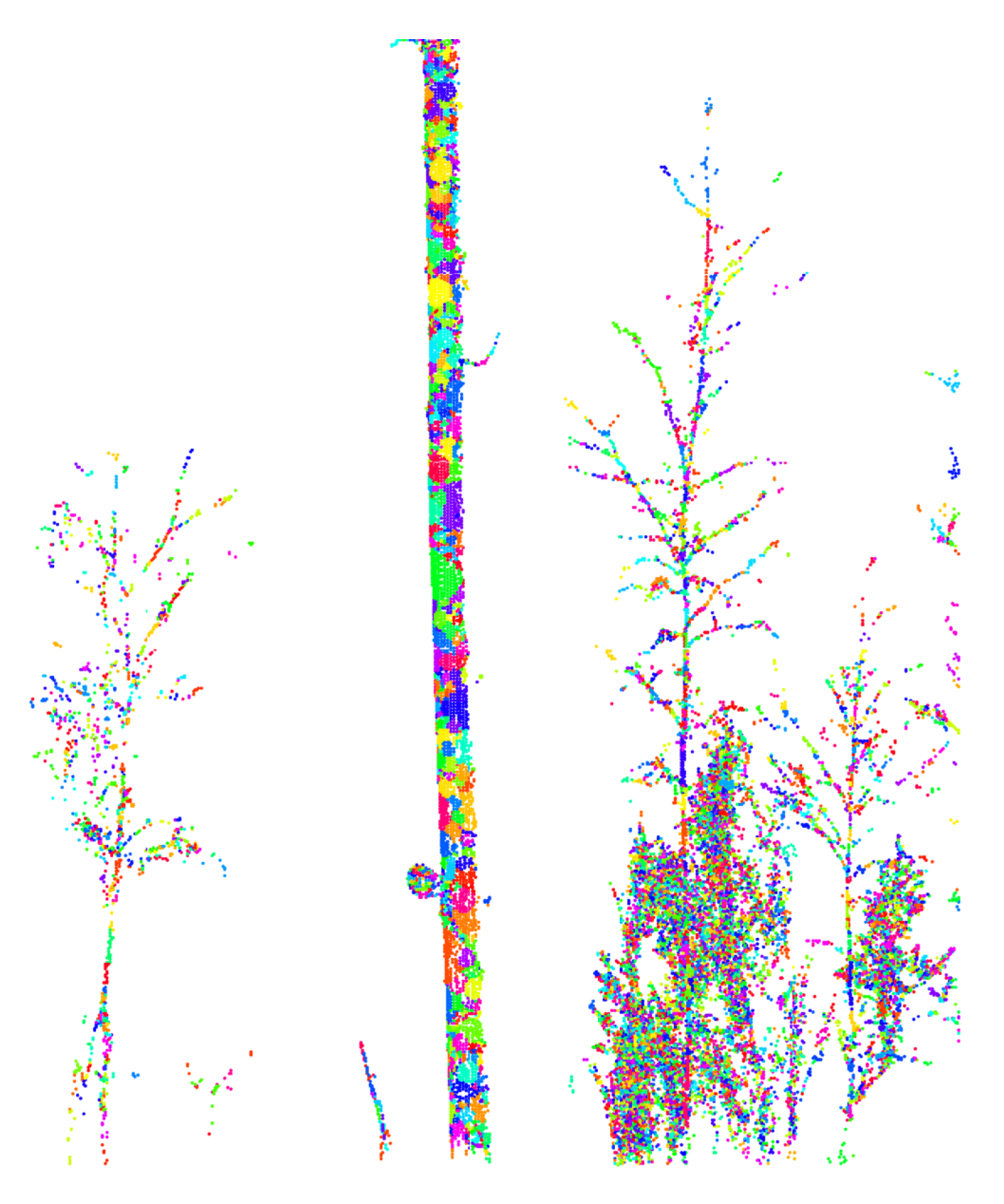
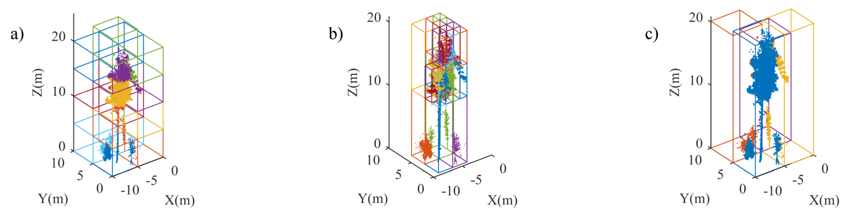
3.1. Dynamic Segment Merging
3.1.1. Normal Vector
3.1.2. Initial Segmentation
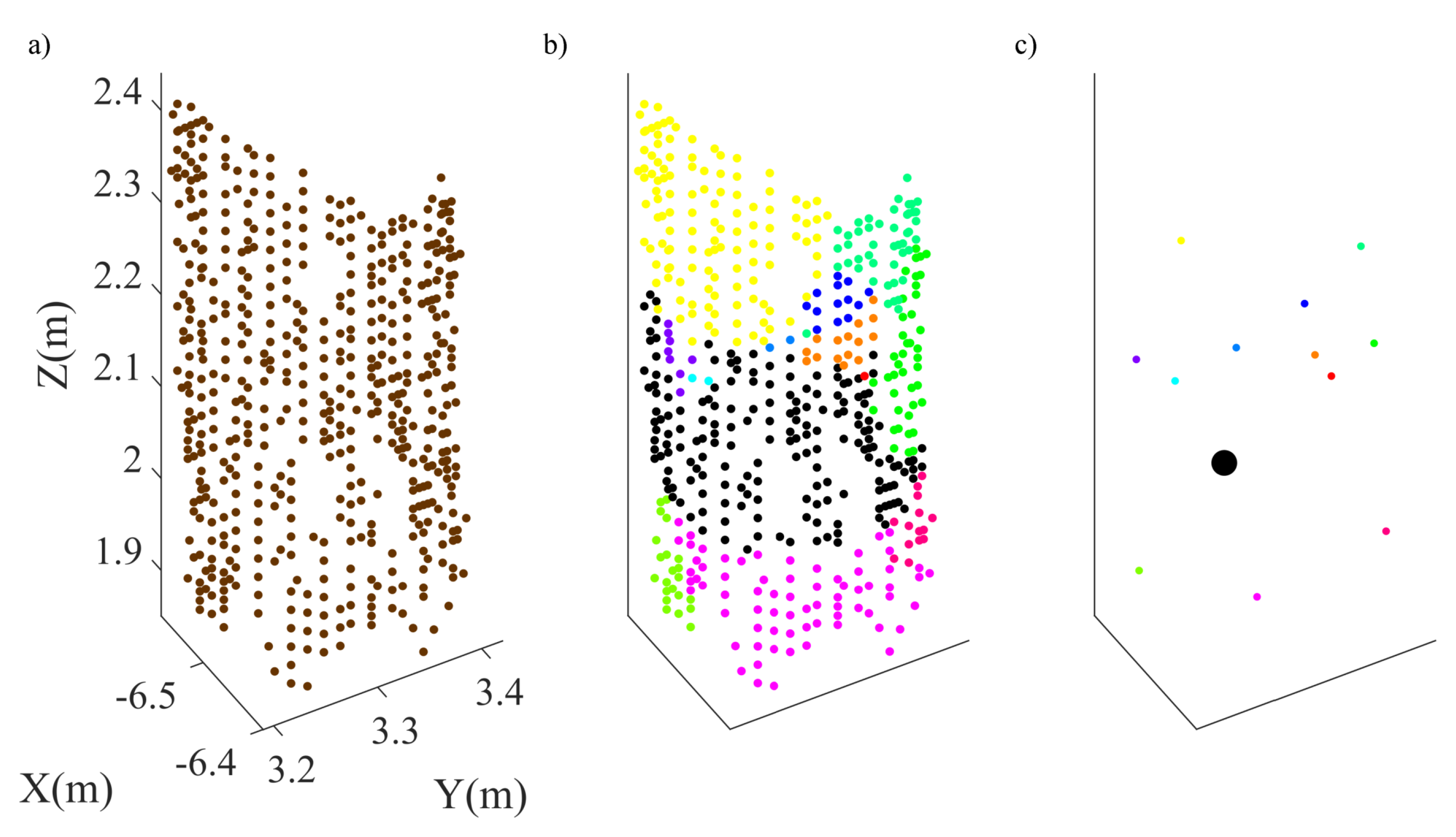
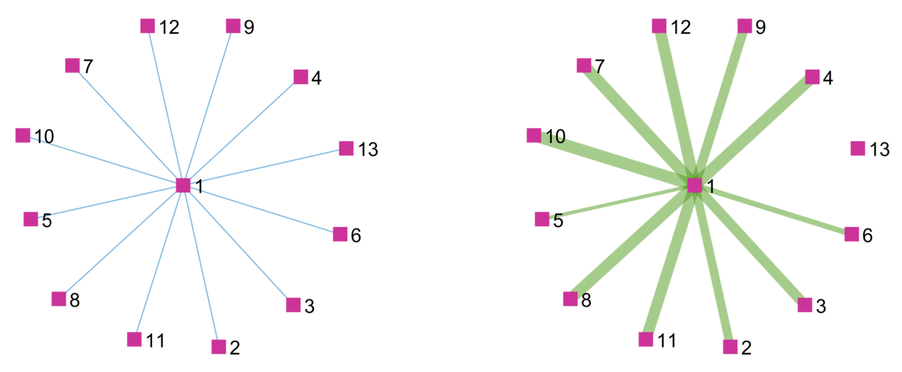
3.1.3. Dynamic Merging
3.2. Post Processing
3.3. Segment Feature
3.4. Tile Processing
3.5. Random Forest Classification
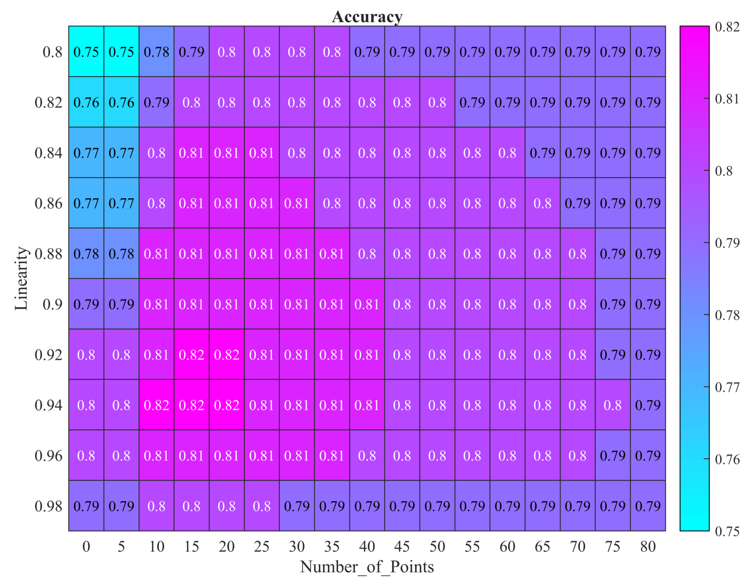
3.6. Evaluation
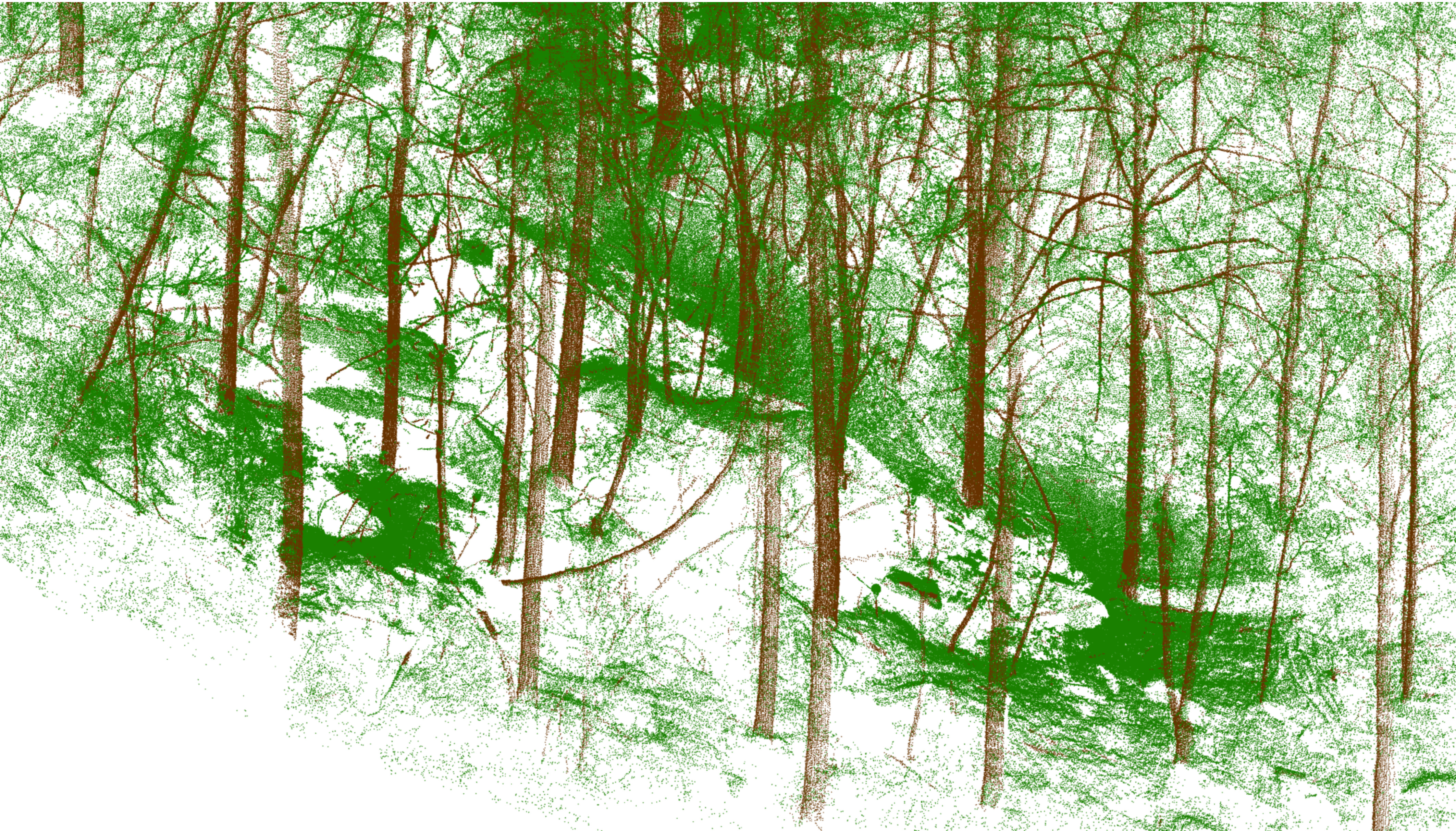
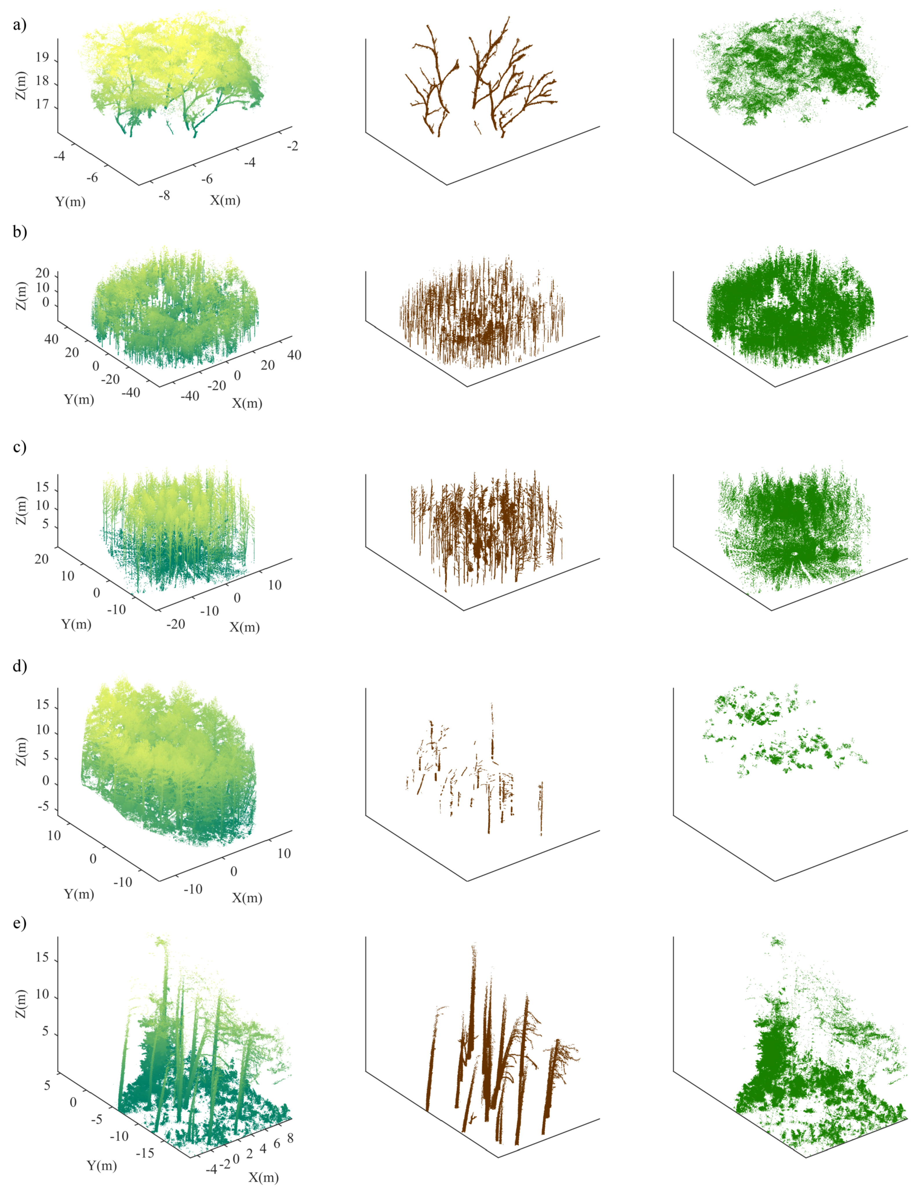
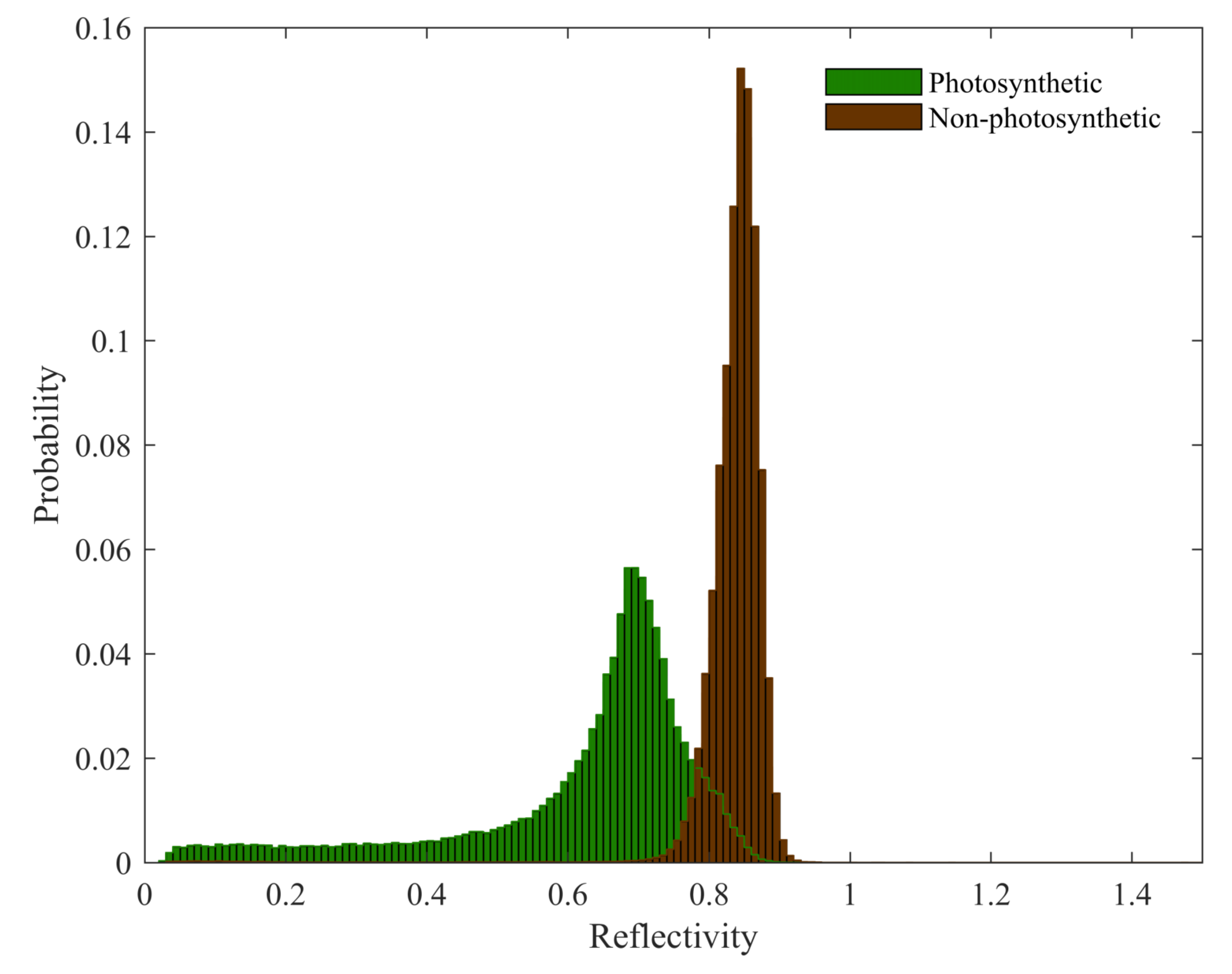
4. Results
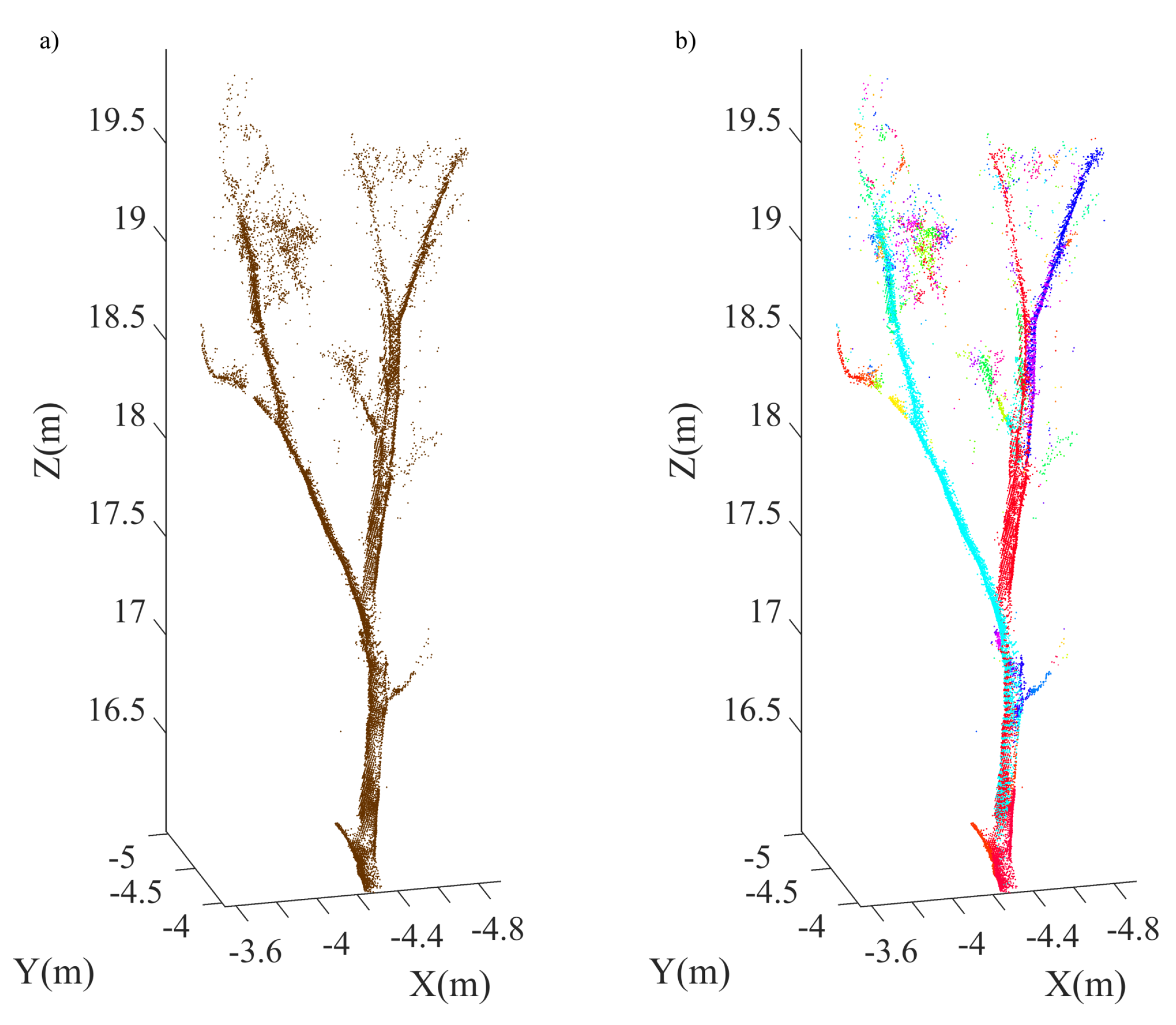
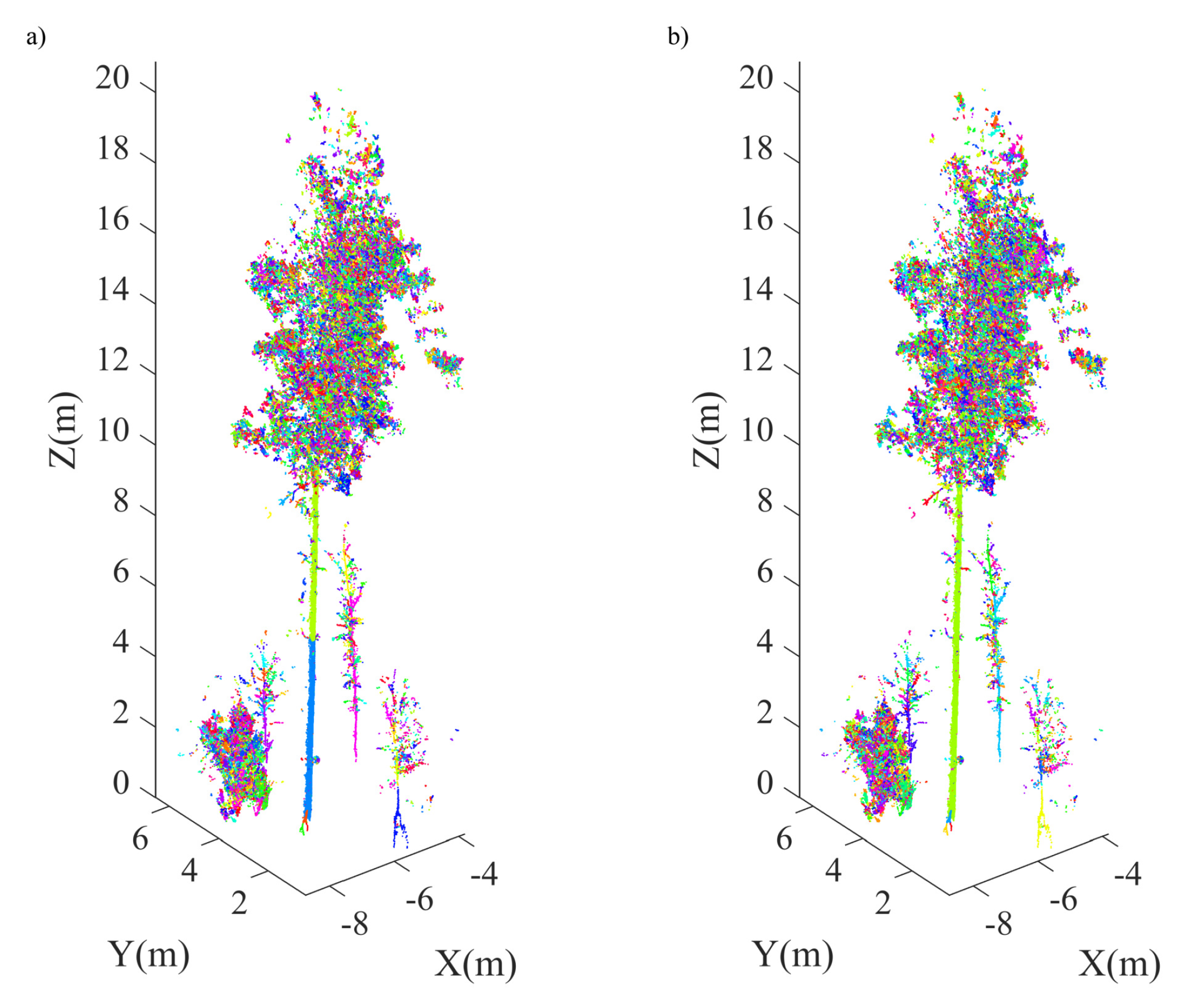
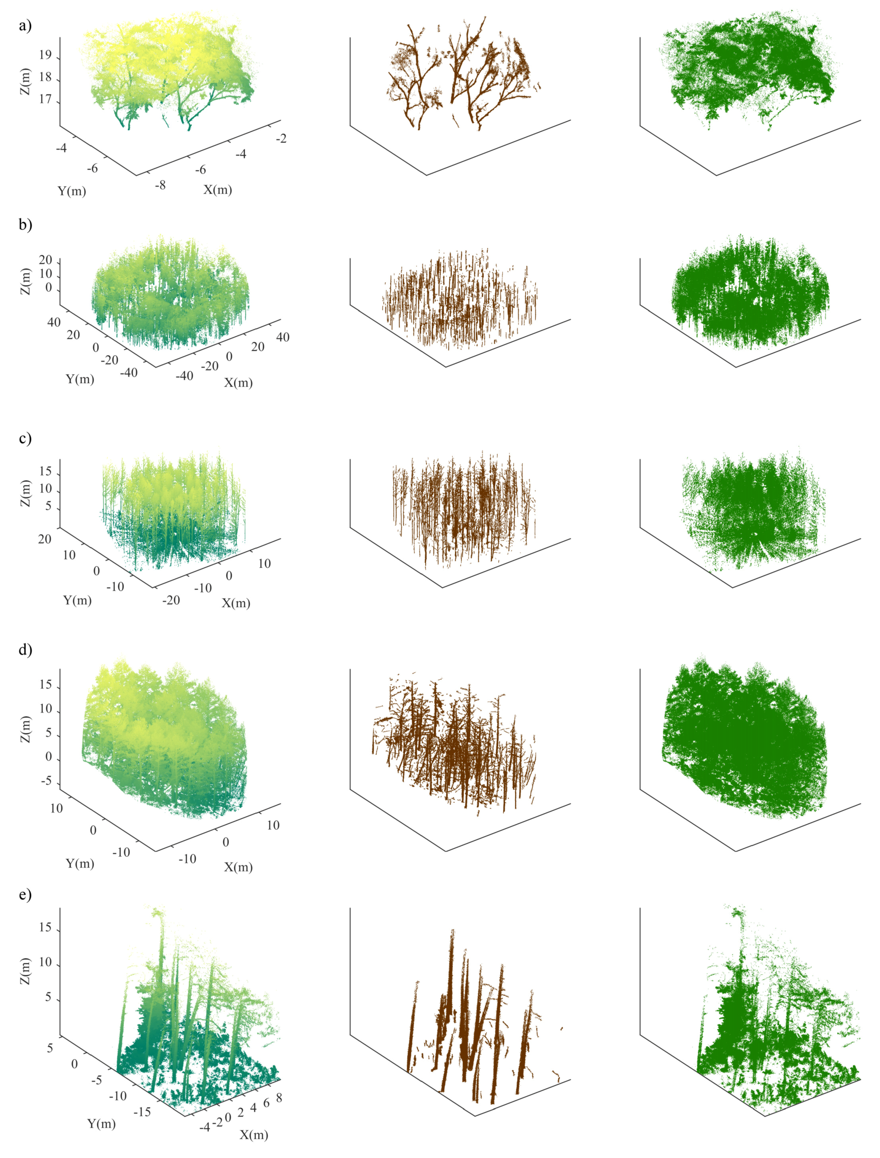
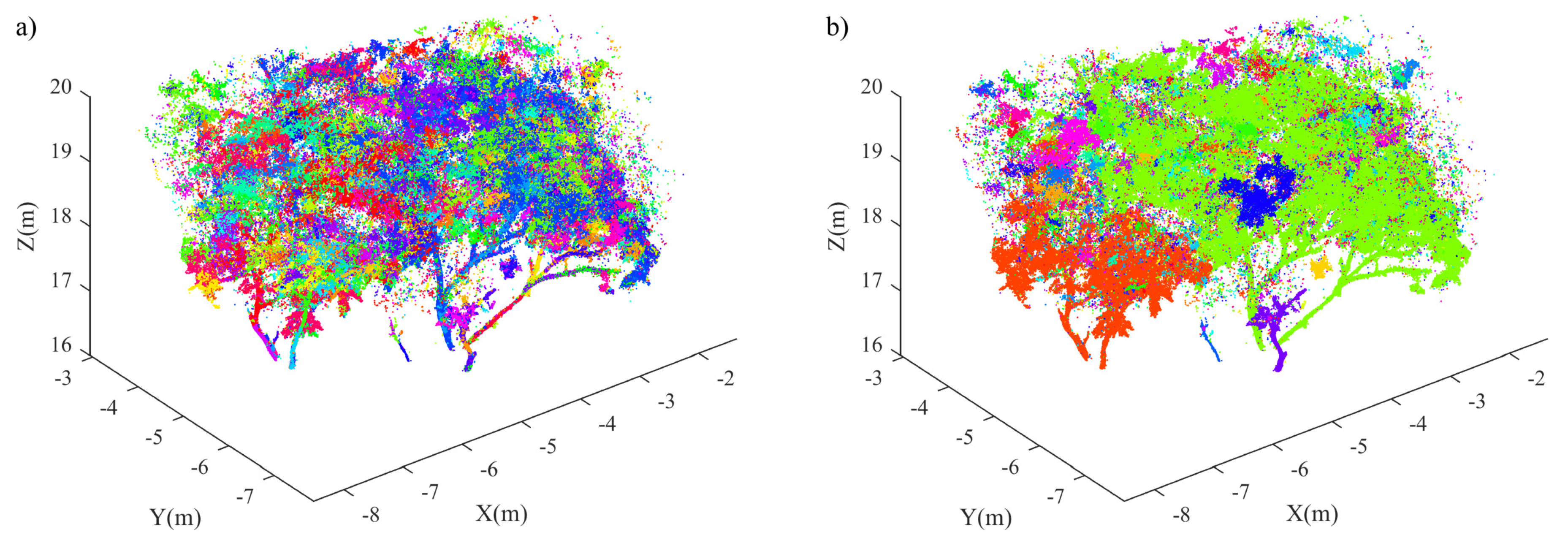
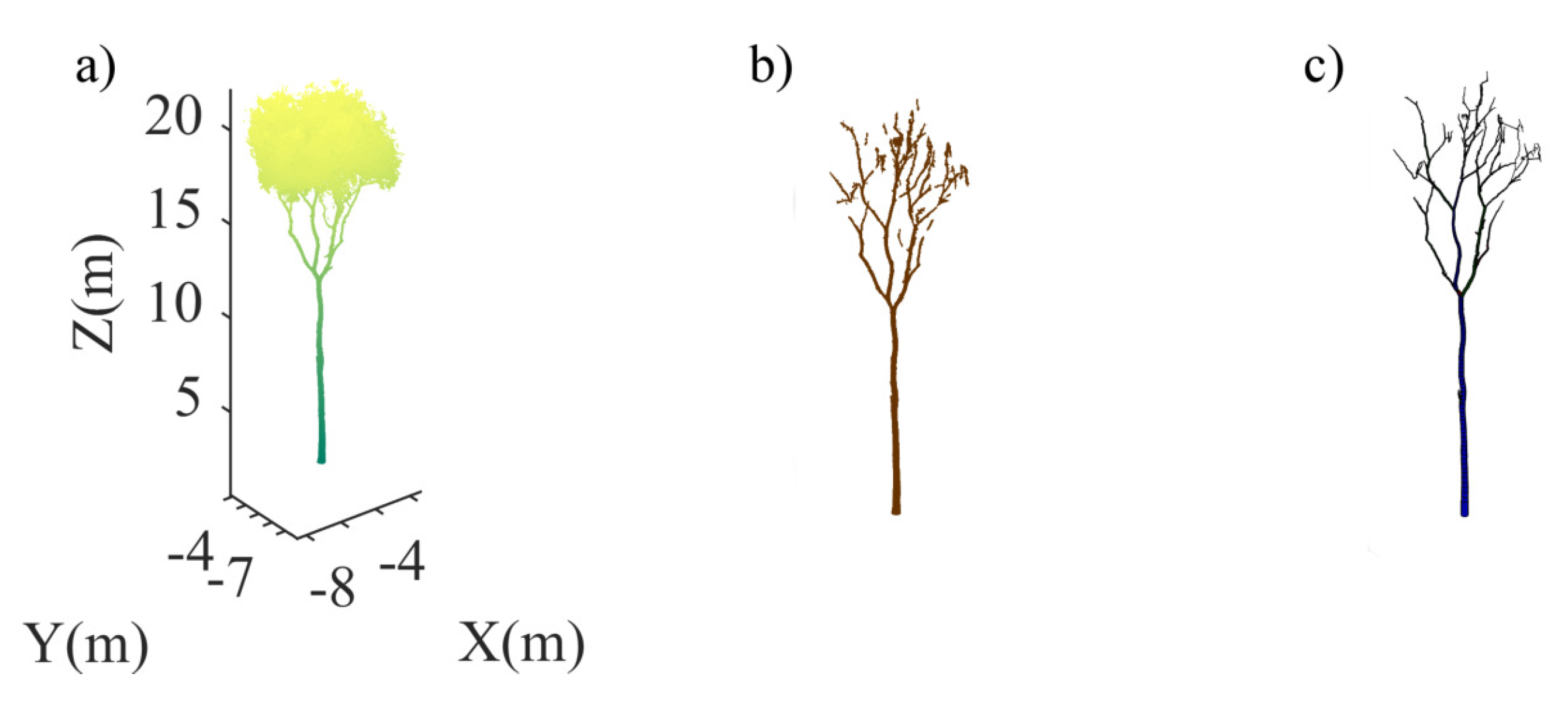
4.1. Single Tree Data
4.2. Plot-Level Data
5. Discussion
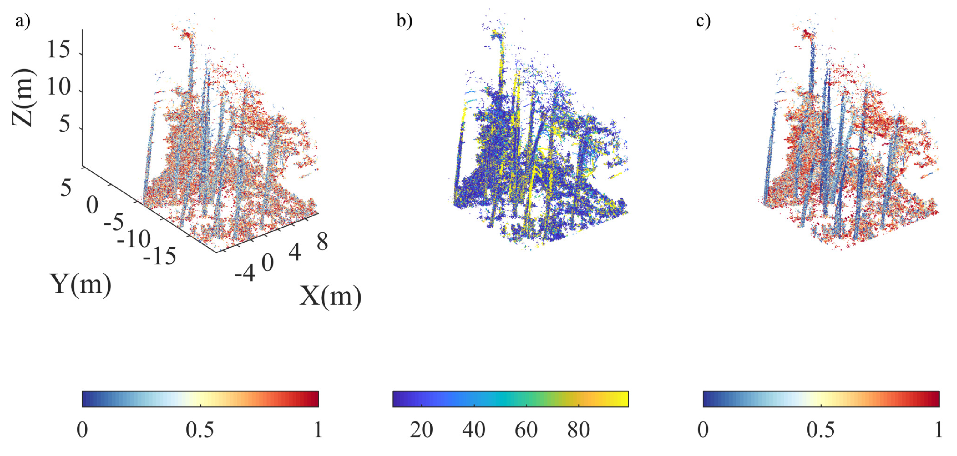
5.1. Calculation of Normal Vectors
5.2. Algorithm Performance
5.3. Challenges in Components Separation
5.4. Future Applications of the DSM Method
6. Conclusions
Author Contributions
Acknowledgments
Conflicts of Interest
References
- Ma, L.; Zheng, G.; Eitel, J.U.; Moskal, L.M.; He, W.; Huang, H. Improved salient feature-based approach for automatically separating photosynthetic and nonphotosynthetic components within terrestrial lidar point cloud data of forest canopies. IEEE Trans. Geosci. Remote Sens. 2016, 54, 679–696. [Google Scholar] [CrossRef]
- Béland, M.; Baldocchi, D.D.; Widlowski, J.L.; Fournier, R.A.; Verstraete, M.M. On seeing the wood from the leaves and the role of voxel size in determining leaf area distribution of forests with terrestrial LiDAR. Agricult. For. Meteorol. 2014, 184, 82–97. [Google Scholar] [CrossRef]
- Levick, S.R.; Hessenmöller, D.; Schulze, E.D. Scaling wood volume estimates from inventory plots to landscapes with airborne LiDAR in temperate deciduous forest. Carbon Balance Manag. 2016, 11, 7. [Google Scholar] [CrossRef] [PubMed]
- Zheng, G.; Moskal, L.M.; Kim, S.H. Retrieval of effective leaf area index in heterogeneous forests with terrestrial laser scanning. IEEE Trans. Geosci. Remote Sens. 2013, 51, 777–786. [Google Scholar] [CrossRef]
- Calders, K.; Newnham, G.; Burt, A.; Murphy, S.; Raumonen, P.; Herold, M.; Culvenor, D.; Avitabile, V.; Disney, M.; Armston, J.; et al. Nondestructive estimates of above-ground biomass using terrestrial laser scanning. Methods Ecol. Evol. 2015, 6, 198–208. [Google Scholar] [CrossRef]
- Chen, J.M.; Black, T. Defining leaf area index for non-flat leaves. Plant Cell Environ. 1992, 15, 421–429. [Google Scholar] [CrossRef]
- Asner, G.P.; Scurlock, J.M.; A Hicke, J. Global synthesis of leaf area index observations: Implications for ecological and remote sensing studies. Glob. Ecol. Biogeogr. 2003, 12, 191–205. [Google Scholar] [CrossRef]
- Li, S.; Dai, L.; Wang, H.; Wang, Y.; He, Z.; Lin, S. Estimating leaf area density of individual trees using the point cloud segmentation of terrestrial LiDAR data and a voxel-based model. Remote Sens. 2017, 9, 1202. [Google Scholar] [CrossRef]
- Wang, D.; Hollaus, M.; Puttonen, E.; Pfeifer, N. Automatic and self-adaptive stem reconstruction in landslide-affected forests. Remote Sens. 2016, 8, 974. [Google Scholar] [CrossRef]
- Liang, X.; Kankare, V.; Yu, X.; Hyyppä, J.; Holopainen, M. Automated stem curve measurement using terrestrial laser scanning. IEEE Trans. Geosci. Remote Sens. 2014, 52, 1739–1748. [Google Scholar] [CrossRef]
- Liang, X.; Kankare, V.; Hyyppä, J.; Wang, Y.; Kukko, A.; Haggrén, H.; Yu, X.; Kaartinen, H.; Jaakkola, A.; Guan, F.; et al. Terrestrial laser scanning in forest inventories. ISPRS J. Photogramm. Remote Sens. 2016, 115, 63–77. [Google Scholar] [CrossRef]
- Maas, H.; Bienert, A.; Scheller, S.; Keane, E. Automatic forest inventory parameter determination from terrestrial laser scanner data. Int. J. Remote Sens. 2008, 29, 1579–1593. [Google Scholar] [CrossRef]
- Liang, X.; Litkey, P.; Hyyppä, J.; Kaartinen, H.; Vastaranta, M.; Holopainen, M. Automatic stem mapping using single-scan terrestrial laser scanning. IEEE Trans. Geosci. Remote Sens. 2012, 50, 661–670. [Google Scholar] [CrossRef]
- You, L.; Tang, S.; Song, X.; Lei, Y.; Zang, H.; Lou, M.; Zhuang, C. Precise measurement of stem diameter by simulating the path of diameter tape from terrestrial laser scanning data. Remote Sens. 2016, 8, 717. [Google Scholar] [CrossRef]
- Chen, Q.; Gong, P.; Baldocchi, D.; Tian, Y.Q. Estimating basal area and stem volume for individual trees from lidar data. Photogramm. Eng. Remote Sens. 2007, 73, 1355–1365. [Google Scholar] [CrossRef]
- Feliciano, E.A.; Wdowinski, S.; Potts, M.D. Assessing mangrove above-ground biomass and structure using terrestrial laser scanning: A case study in the Everglades National Park. Wetlands 2014, 34, 955–968. [Google Scholar] [CrossRef]
- Tao, S.; Guo, Q.; Su, Y.; Xu, S.; Li, Y.; Wu, F. A geometric method for wood-leaf separation using terrestrial and simulated lidar data. Photogramm. Eng. Remote Sens. 2015, 81, 767–776. [Google Scholar] [CrossRef]
- Yun, T.; An, F.; Li, W.; Sun, Y.; Cao, L.; Xue, L. A novel approach for retrieving tree leaf area from ground-based LiDAR. Remote Sens. 2016, 8, 942. [Google Scholar] [CrossRef]
- Pfennigbauer, M.; Ullrich, A. Improving quality of laser scanning data acquisition through calibrated amplitude and pulse deviation measurement. SPIE Def. Secur. Sens. Int. Soc. Opt. Photonics 2010, 7684, 76841F. [Google Scholar]
- Disney, M.I.; Boni Vicari, M.; Burt, A.; Calders, K.; Lewis, S.L.; Raumonen, P.; Wilkes, P. Weighing trees with lasers: Advances, challenges and opportunities. Interface Focus 2018, 8. [Google Scholar] [CrossRef] [PubMed]
- Zhu, X.; Skidmore, A.K.; Darvishzadeh, R.; Niemann, K.O.; Liu, J.; Shi, Y.; Wang, T. Foliar and woody materials discriminated using terrestrial LiDAR in a mixed natural forest. Int. J. Appl. Earth Observ. Geoinf. 2018, 64, 43–50. [Google Scholar] [CrossRef]
- Kaasalainen, S.; Krooks, A.; Kukko, A.; Kaartinen, H. Radiometric calibration of terrestrial laser scanners with external reference targets. Remote Sens. 2009, 1, 144–158. [Google Scholar] [CrossRef]
- Calders, K.; Disney, M.I.; Armston, J.; Burt, A.; Brede, B.; Origo, N.; Muir, J.; Nightingale, J. Evaluation of the Range Accuracy and the Radiometric Calibration of Multiple Terrestrial Laser Scanning Instruments for Data Interoperability. IEEE Trans. Geosci. Remote Sens. 2017, 55, 2716–2724. [Google Scholar] [CrossRef]
- Höfle, B.; Pfeifer, N. Correction of laser scanning intensity data: Data and model-driven approaches. ISPRS J. Photogramm. Remote Sens. 2007, 62, 415–433. [Google Scholar] [CrossRef]
- Kaasalainen, S.; Jaakkola, A.; Kaasalainen, M.; Krooks, A.; Kukko, A. Analysis of incidence angle and distance effects on terrestrial laser scanner intensity: Search for correction methods. Remote Sens. 2011, 3, 2207–2221. [Google Scholar] [CrossRef]
- Li, Z.; Douglas, E.; Strahler, A.; Schaaf, C.; Yang, X.; Wang, Z.; Yao, T.; Zhao, F.; Saenz, E.J.; Paynter, I.; et al. Separating leaves from trunks and branches with dual-wavelength terrestrial LiDAR scanning. In Proceedings of the 2013 IEEE International Conference on Geoscience and Remote Sensing Symposium (IGARSS), Melbourne, Australia, 21–26 July 2013; pp. 3383–3386. [Google Scholar]
- Hakala, T.; Suomalainen, J.; Kaasalainen, S.; Chen, Y. Full waveform hyperspectral LiDAR for terrestrial laser scanning. Opt. Express 2012, 20, 7119–7127. [Google Scholar] [CrossRef] [PubMed]
- Vauhkonen, J.; Hakala, T.; Suomalainen, J.; Kaasalainen, S.; Nevalainen, O.; Vastaranta, M.; Holopainen, M.; Hyyppä, J. Classification of spruce and pine trees using active hyperspectral LiDAR. IEEE Geosci. Remote Sens. Lett. 2013, 10, 1138–1141. [Google Scholar] [CrossRef]
- Belton, D.; Moncrieff, S.; Chapman, J. Processing tree point clouds using Gaussian mixture models. In Proceedings of the ISPRS Annals of the Photogrammetry, Remote Sensing and Spatial Information Sciences, Antalya, Turkey, 11–13 November 2013; pp. 11–13. [Google Scholar]
- Wang, D.; Hollaus, M.; Pfeifer, N. Feasibility of machine learning methods for separating wood and leaf points from terrestrial laser scanning data. ISPRS Ann. Photogramm. Remote Sens. Spat. Inf. Sci. 2017, IV-2/W4, 157–164. [Google Scholar] [CrossRef]
- Zhang, W.; Qi, J.; Wan, P.; Wang, H.; Xie, D.; Wang, X.; Yan, G. An easy-to-use airborne LiDAR data filtering method based on cloth simulation. Remote Sens. 2016, 8, 501. [Google Scholar] [CrossRef]
- Hackenberg, J.; Wassenberg, M.; Spiecker, H.; Sun, D. Non destructive method for biomass prediction combining TLS derived tree volume and wood density. Forests 2015, 6, 1274–1300. [Google Scholar] [CrossRef]
- Hyyppä, J.; Liang, X. Project Benchmarking on Terrestrial Laser Scanning for Forestry Applications. Available online: http://www.eurosdr.net/research/project/project-benchmarking-terrestrial-laser-scanning-forestry-applications (accessed on 18 February 2018).
- Adams, R.; Bischof, L. Seeded region growing. IEEE Trans. Pattern Anal. Mach. Intell. 1994, 16, 641–647. [Google Scholar] [CrossRef]
- Huang, Z.; Zhang, J.; Li, X.; Zhang, H. Remote sensing image segmentation based on dynamic statistical region merging. Optik Int. J. Light Electron Opt. 2014, 125, 870–875. [Google Scholar] [CrossRef]
- Landrieu, L.; Simonovsky, M. Large-scale point cloud semantic segmentation with superpoint graphs. arXiv, 2017; arXiv:1711.09869. [Google Scholar]
- Peng, B.; Zhang, L.; Zhang, D. Automatic image segmentation by dynamic region merging. IEEE Trans. Image Process. 2011, 20, 3592–3605. [Google Scholar] [CrossRef] [PubMed]
- Rabbani, T.; Van Den Heuvel, F.; Vosselmann, G. Segmentation of point clouds using smoothness constraint. Int. Arch. Photogramm. Remote Sens. Spat. Inf. Sci. 2006, 36, 248–253. [Google Scholar]
- Höfle, B. Radiometric correction of terrestrial LiDAR point cloud data for individual maize plant detection. IEEE Geosci. Remote Sens. Lett. 2014, 11, 94–98. [Google Scholar] [CrossRef]
- Lari, Z.; Habib, A.; Kwak, E. An adaptive approach for segmentation of 3D laser point cloud. ISPRS Workshop Laser Scanning 2011, XXXVIII-5/W12, 29–31. [Google Scholar] [CrossRef]
- Klasing, K.; Althoff, D.; Wollherr, D.; Buss, M. Comparison of surface normal estimation methods for range sensing applications. In Proceedings of the IEEE International Conference on Robotics and Automation (ICRA’09), Kobe, Japan, 12–17 May 2009; pp. 3206–3211. [Google Scholar]
- Liu, M.; Pomerleau, F.; Colas, F.; Siegwart, R. Normal estimation for pointcloud using GPU based sparse tensor voting. In Proceedings of the 2012 IEEE International Conference on Robotics and Biomimetics (ROBIO), Guangzhou, China, 11–14 December 2012; pp. 91–96. [Google Scholar]
- Garland, M. Quadric-Based Polygonal Surface Simplification; Technical Report; School of Computer Science, Carnegie Mellon University: Pittsburgh, PA, USA, 1999. [Google Scholar]
- Bazazian, D.; Casas, J.R.; Ruiz-Hidalgo, J. Fast and robust edge extraction in unorganized point clouds. In Proceedings of the 2015 International Conference on Digital Image Computing: Techniques and Applications (DICTA), Adelaide, Australia, 23–25 November 2015; pp. 1–8. [Google Scholar]
- Weinmann, M.; Jutzi, B.; Mallet, C. Semantic 3D scene interpretation: A framework combining optimal neighborhood size selection with relevant features. ISPRS Ann. Photogramm. Remote Sens. Spat. Inf. Sci. 2014, 2, 181. [Google Scholar] [CrossRef]
- Chen, M.; Wan, Y.; Wang, M.; Xu, J. Automatic stem detection in terrestrial laser scanning data with distance-adaptive search radius. IEEE Trans. Geosci. Remote Sens. 2018, 56, 2968–2979. [Google Scholar] [CrossRef]
- Xia, S.; Wang, C.; Pan, F.; Xi, X.; Zeng, H.; Liu, H. Detecting stems in dense and homogeneous forest using single-scan TLS. Forests 2015, 6, 3923–3945. [Google Scholar] [CrossRef]
- Brodu, N.; Lague, D. 3D terrestrial lidar data classification of complex natural scenes using a multi-scale dimensionality criterion: Applications in geomorphology. ISPRS J. Photogramm. Remote Sens. 2012, 68, 121–134. [Google Scholar] [CrossRef]
- Kaick, O.V.; Fish, N.; Kleiman, Y.; Asafi, S.; Cohen-Or, D. Shape segmentation by approximate convexity analysis. ACM Trans. Graph. 2014, 34, 4. [Google Scholar] [CrossRef]
- Vosselman, G.; Coenen, M.; Rottensteiner, F. Contextual segment-based classification of airborne laser scanner data. ISPRS J. Photogramm. Remote Sens. 2017, 128, 354–371. [Google Scholar] [CrossRef]
- Hackel, T.; Wegner, J.D.; Schindler, K. Fast semantic segmentation of 3D point clouds with strongly varying density. ISPRS Ann. Photogramm. Remote Sens. Spat. Inf. Sci. 2016, III-3, 177–184. [Google Scholar] [CrossRef]
- Raumonen, P.; Kaasalainen, M.; Åkerblom, M.; Kaasalainen, S.; Kaartinen, H.; Vastaranta, M.; Holopainen, M.; Disney, M.; Lewis, P. Fast automatic precision tree models from terrestrial laser scanner data. Remote Sens. 2013, 5, 491–520. [Google Scholar] [CrossRef]
- Pöchtrager, M.; Styhler-Aydin, G.; Döring-Williams, M.; Pfeifer, N. Automated reconstruction of historic roof structures from point clouds-development and examples. ISPRS Ann. Photogramm. Remote Sens. Spat. Inf. Sci. 2017, IV-2/W2, 195–202. [Google Scholar]
- Filin, S.; Pfeifer, N. Neighborhood systems for airborne laser data. Photogramm. Eng. Remote Sens. 2005, 71, 743–755. [Google Scholar] [CrossRef]
- Comaniciu, D.; Meer, P. Mean shift: A robust approach toward feature space analysis. IEEE Trans. Pattern Anal. Mach. Intell. 2002, 24, 603–619. [Google Scholar] [CrossRef]
- Pfeifer, N.; Mandlburger, G.; Otepka, J.; Karel, W. OPALS—A framework for Airborne Laser Scanning data analysis. Comput. Environ. Urban Syst. 2014, 45, 125–136. [Google Scholar] [CrossRef]
- Vosselman, G. Point cloud segmentation for urban scene classification. Int. Arch. Photogramm. Remote Sens. Spat. Inf. Sci. 2013, 1, 257–262. [Google Scholar] [CrossRef]
- Papon, J.; Abramov, A.; Schoeler, M.; Wörgötter, F. Voxel cloud connectivity segmentation-supervoxels for point clouds. In Proceedings of the 2013 IEEE Conference on Computer Vision and Pattern Recognition (CVPR), Portland, OR, USA, 23–28 June 2013; pp. 2027–2034. [Google Scholar]
- Breiman, L. Random forests. Machine learning 2001, 45, 5–32. [Google Scholar] [CrossRef]
- Weinmann, M.; Urban, S.; Hinz, S.; Jutzi, B.; Mallet, C. Distinctive 2D and 3D features for automated large-scale scene analysis in urban areas. Comput. Graph. 2015, 49, 47–57. [Google Scholar] [CrossRef]
- Qi, C.R.; Su, H.; Mo, K.; Guibas, L.J. Pointnet: Deep learning on point sets for 3d classification and segmentation. Comput. Vis. Pattern Recognit. 2017, 1, 4. [Google Scholar]
- Li, Y.; Bu, R.; Sun, M.; Chen, B. PointCNN. arXiv, 2018; arXiv:1801.07791. [Google Scholar]
- Wang, D.; Kankare, V.; Puttonen, E.; Hollaus, M.; Pfeifer, N. Reconstructing stem cross section shapes from terrestrial laser scanning. IEEE Geosci. Remote Sens. Lett. 2017, 14, 272–276. [Google Scholar] [CrossRef]


| No. | Feature | Description |
|---|---|---|
| 1 | linearity | linear saliency . |
| 2 | planarity | planar saliency . |
| 3 | scattering | volumetric saliency . |
| 4 | omnivariance | volume of the neighborhood . |
| 5 | anisotropy | . |
| 6 | eigenentropy | |
| 7 | sum | . |
| 8 | surface_variation | change of curvature . |
| 9 | X value | X coordinate of the point. |
| 10 | Y value | Y coordinate of the point. |
| 11 | Z value | height of the point. |
| 12 | density | local point density. |
| 13 | verticality | . |
| 14 | height difference of local neighborhood. | |
| 15 | standard deviation of heights of local neighborhood. | |
| 16 | z-component of the normal vector . | |
| 17 | radius | radius of local neighborhood. |
| 18 | density | local point density. |
| 19 | sum | . |
| 20 | . | |
| 21 | cell_density | density of projected 2D cells. |
| 22 | skewness | skewness of point heights in each cell. |
| 23 | kurtosis | kurtosis of point heights in each cell. |
| 24 | Max_z | maximum of heights of points in each cell. |
| 25 | Min_z | minimum of heights of points in each cell. |
| 26 | Mean_z | average height of points in each cell. |
| 27 | Median_z | median height of points in each cell. |
| 28 | first eigenvalue of 3D covariance matrix. | |
| 29 | second eigenvalue of 3D covariance matrix. | |
| 30 | third eigenvalue of 3D covariance matrix. | |
| 31 | first eigenvalue of 2D covariance matrix. | |
| 32 | second eigenvalue of 2D covariance matrix. |
| Evaluation | Method | Dataset | ||||
|---|---|---|---|---|---|---|
| SD-1 | PD-1 | PD-2 | PD-3 | PD-4 | ||
| Number of points | 553,556 | 16,259,081 | 2,013,331 | 3,901,367 | 1,269,318 | |
| Number of RF training points * | 86,618 | 117,534 | 53,872 | 59,114 | 31,776 | |
| Number of validation points * | 279,580 | 15,492,926 | 1,648,514 | 77,462 | 945,262 | |
| Sensitivity (%) | DSM(F) | 94.7 | 97.9 | 92.2 | 97.5 | 95.5 |
| DSM(A) | 93.7 | 96.4 | 90.5 | 96.7 | 95.2 | |
| RF(F) | 81.5 | 73.1 | 88.4 | 86.2 | 95.7 | |
| RF(A) | 86.6 | 84.7 | 92.5 | 91.8 | 95.9 | |
| Intensity | – | 92.1 | – | – | – | |
| Specificity (%) | DSM(F) | 79.1 | 74.5 | 64.8 | 81.5 | 76.1 |
| DSM(A) | 83.3 | 81.1 | 73.0 | 87.4 | 79.4 | |
| RF(F) | 82.7 | 92.9 | 77.2 | 97.1 | 70.3 | |
| RF(A) | 81.1 | 87.9 | 74.0 | 95.8 | 73.5 | |
| Intensity | – | 83.1 | – | – | – | |
| Overall accuracy (%) | DSM(F) | 86.9 | 86.2 | 78.5 | 89.5 | 85.8 |
| DSM(A) | 88.5 | 88.7 | 81.8 | 92.0 | 87.3 | |
| RF(F) | 82.1 | 83.0 | 82.8 | 91.7 | 83.0 | |
| RF(A) | 83.9 | 86.3 | 83.2 | 93.8 | 84.7 | |
| Intensity | – | 87.6 | – | – | – | |
© 2018 by the authors. Licensee MDPI, Basel, Switzerland. This article is an open access article distributed under the terms and conditions of the Creative Commons Attribution (CC BY) license (http://creativecommons.org/licenses/by/4.0/).
Share and Cite
Wang, D.; Brunner, J.; Ma, Z.; Lu, H.; Hollaus, M.; Pang, Y.; Pfeifer, N. Separating Tree Photosynthetic and Non-Photosynthetic Components from Point Cloud Data Using Dynamic Segment Merging. Forests 2018, 9, 252. https://doi.org/10.3390/f9050252
Wang D, Brunner J, Ma Z, Lu H, Hollaus M, Pang Y, Pfeifer N. Separating Tree Photosynthetic and Non-Photosynthetic Components from Point Cloud Data Using Dynamic Segment Merging. Forests. 2018; 9(5):252. https://doi.org/10.3390/f9050252
Chicago/Turabian StyleWang, Di, Jasmin Brunner, Zhenyu Ma, Hao Lu, Markus Hollaus, Yong Pang, and Norbert Pfeifer. 2018. "Separating Tree Photosynthetic and Non-Photosynthetic Components from Point Cloud Data Using Dynamic Segment Merging" Forests 9, no. 5: 252. https://doi.org/10.3390/f9050252
APA StyleWang, D., Brunner, J., Ma, Z., Lu, H., Hollaus, M., Pang, Y., & Pfeifer, N. (2018). Separating Tree Photosynthetic and Non-Photosynthetic Components from Point Cloud Data Using Dynamic Segment Merging. Forests, 9(5), 252. https://doi.org/10.3390/f9050252