Predicting Potential Fire Severity Using Vegetation, Topography and Surface Moisture Availability in a Eurasian Boreal Forest Landscape


Abstract
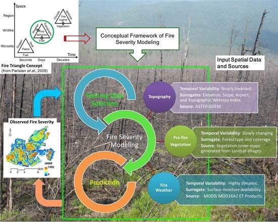
1. Introduction
2. Materials and Methods
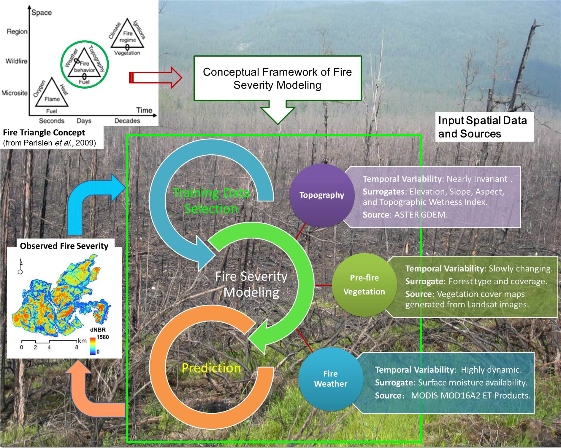
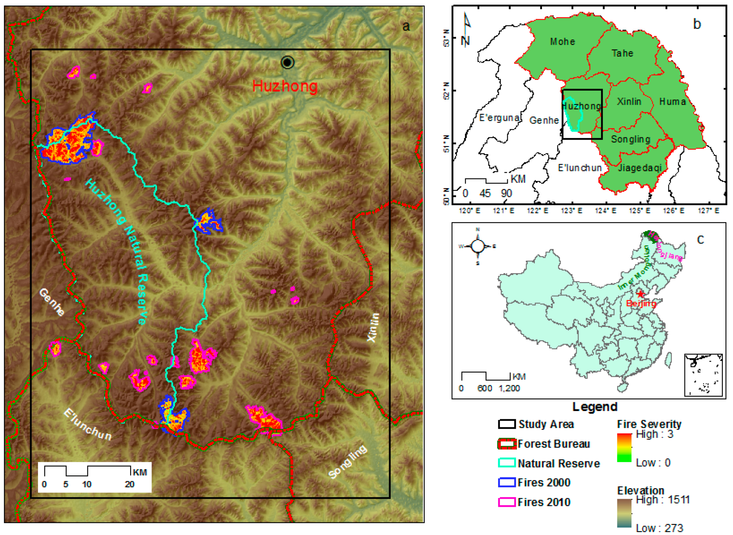
2.1. Study Area
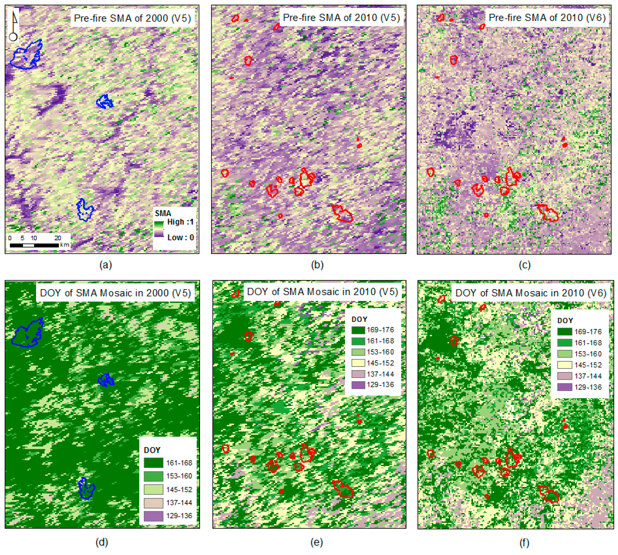
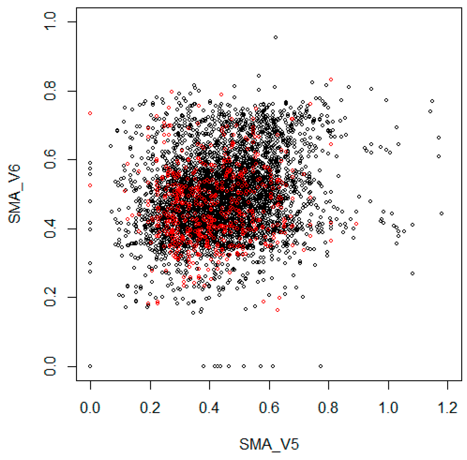
2.2. Remote Sensing Imagery Processing
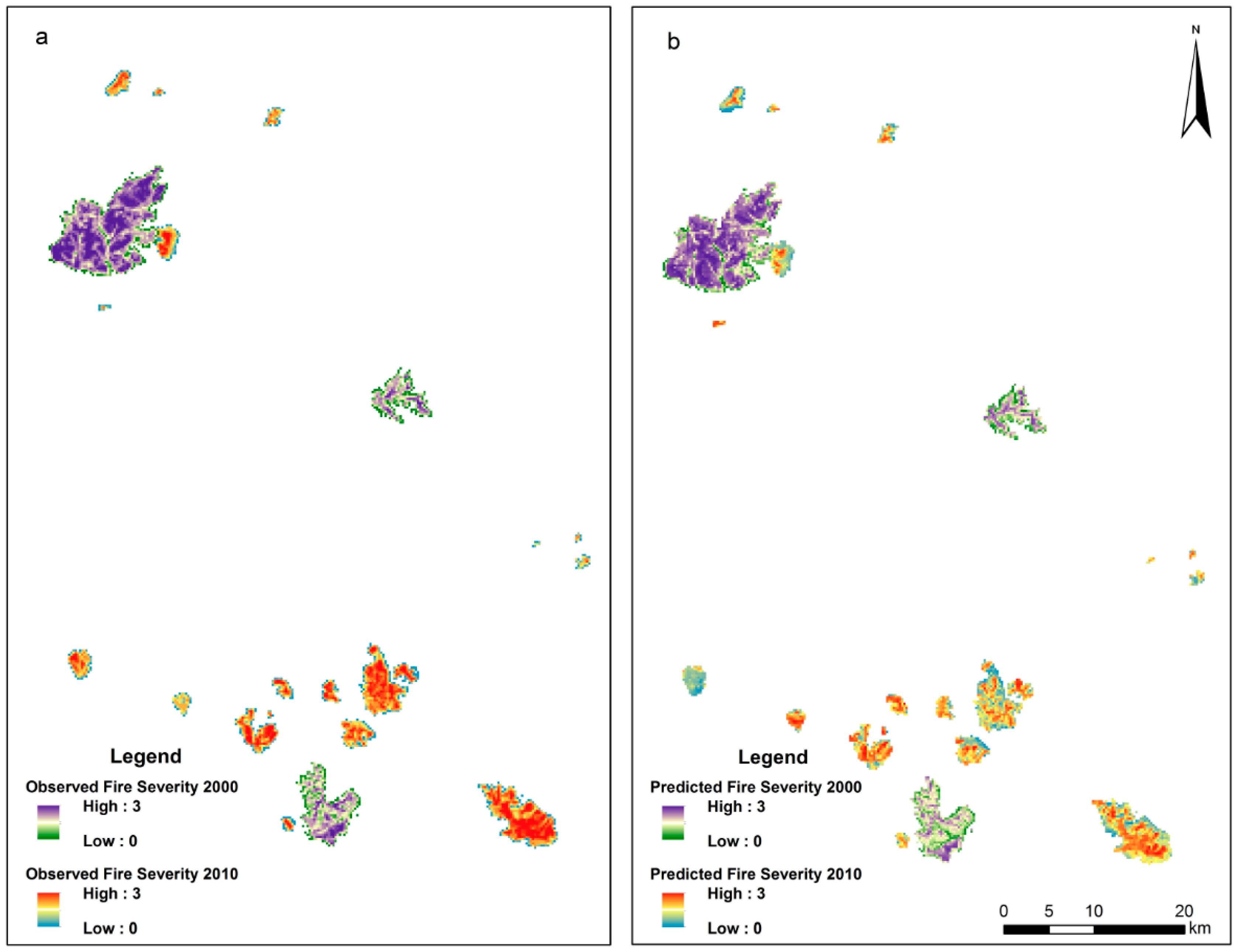
2.3. Fire Severity Mapping
2.4. Environmental Metrics
2.5. Spatial Data Processing
2.6. Statistical Modeling
3. Results
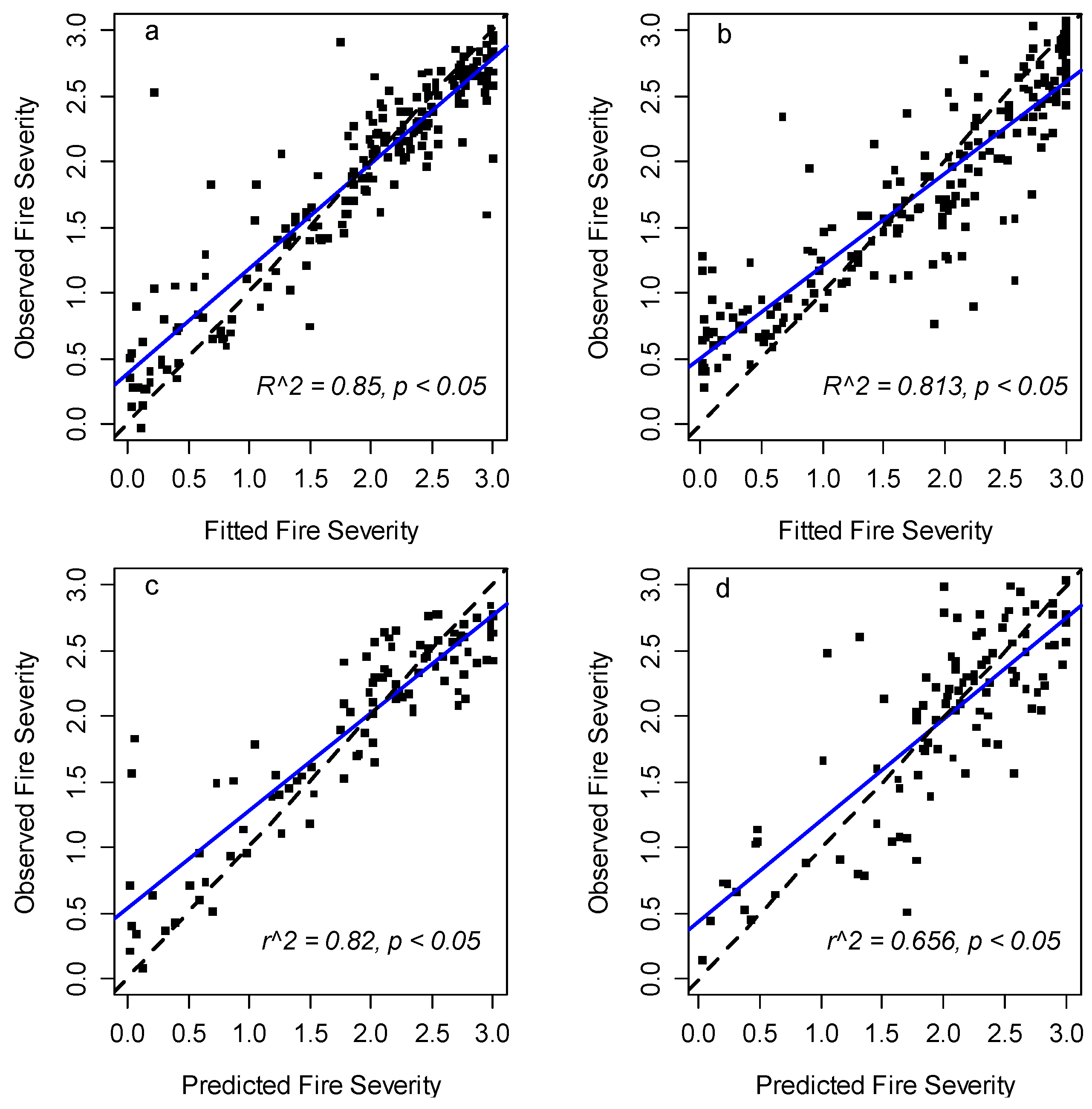
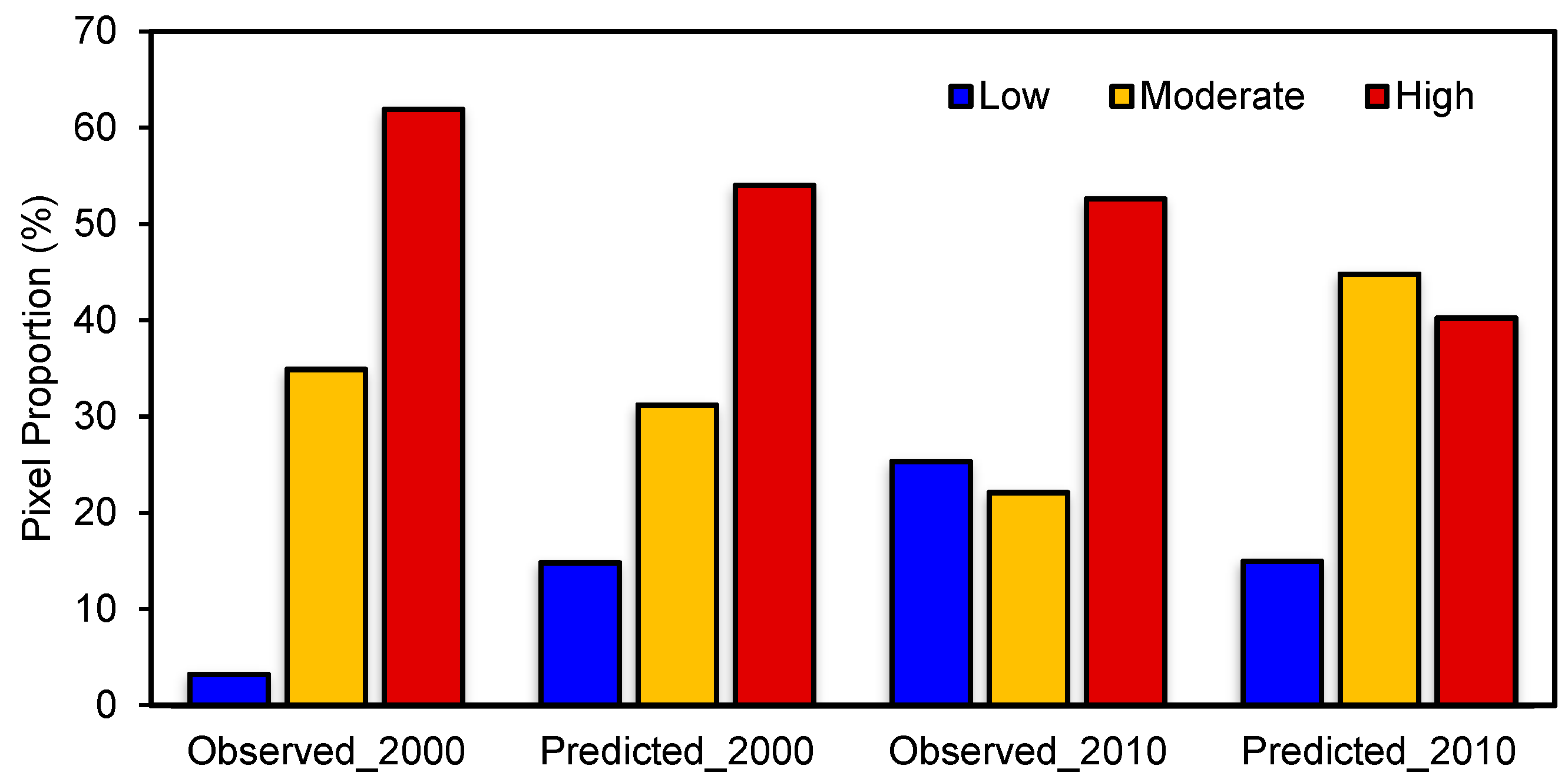
3.1. Evaluation of Model Performance
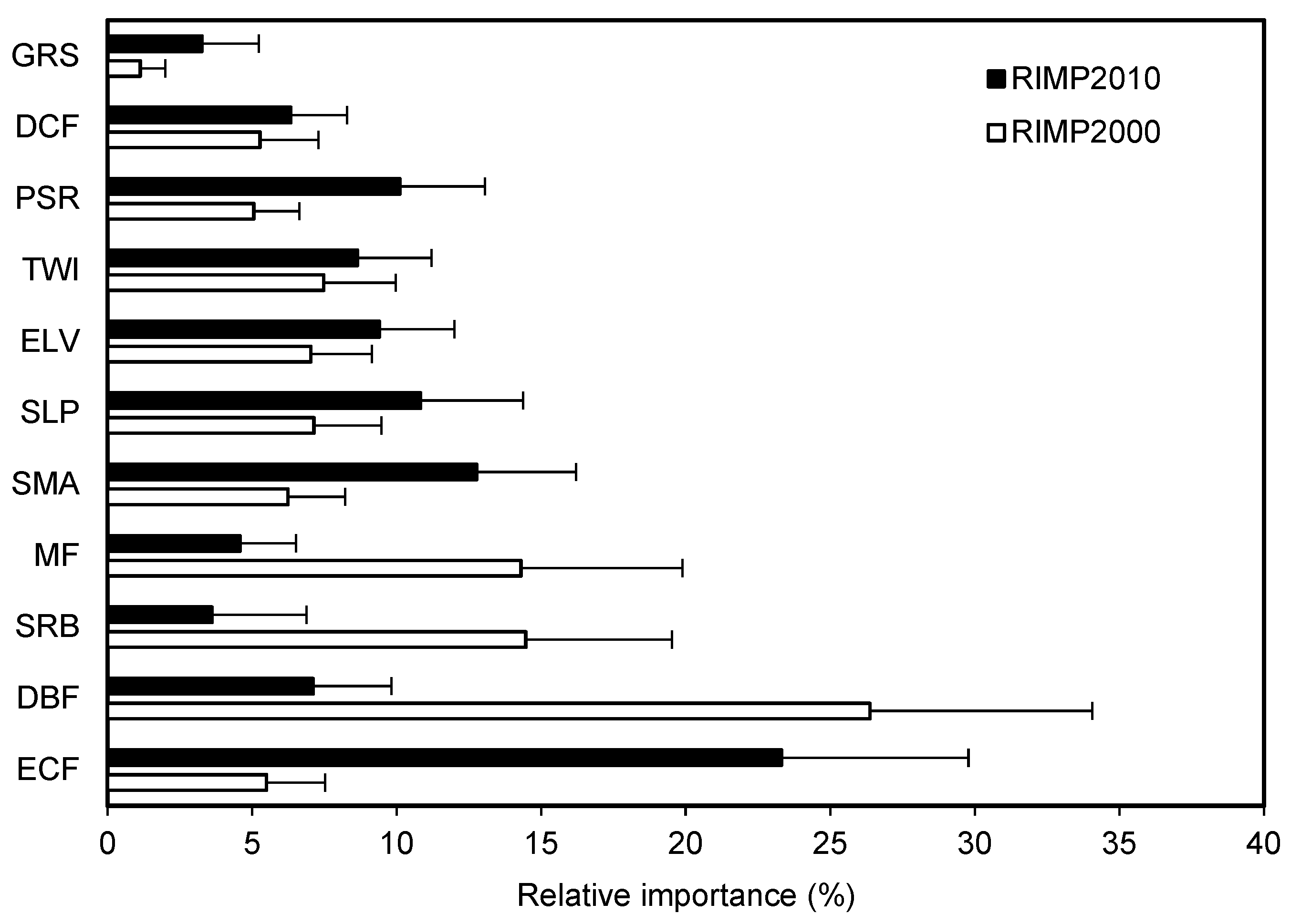
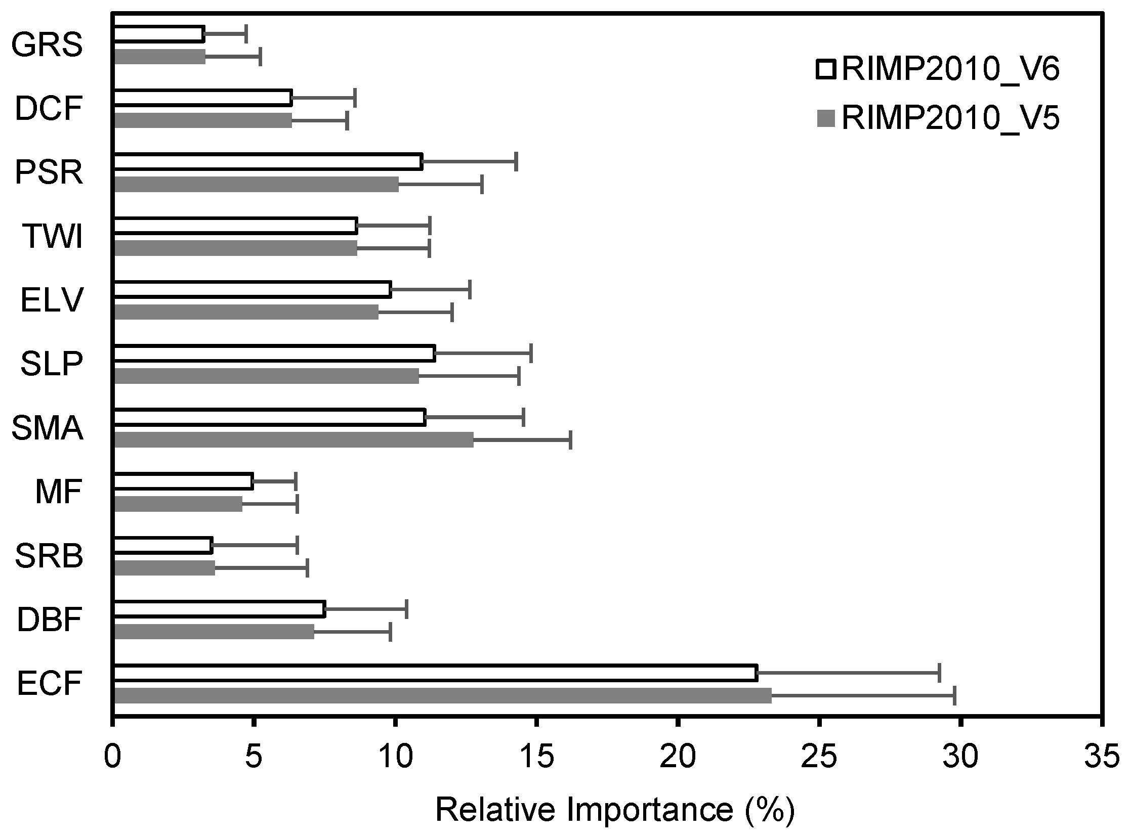
3.2. Relative Importance of Environmental Variables
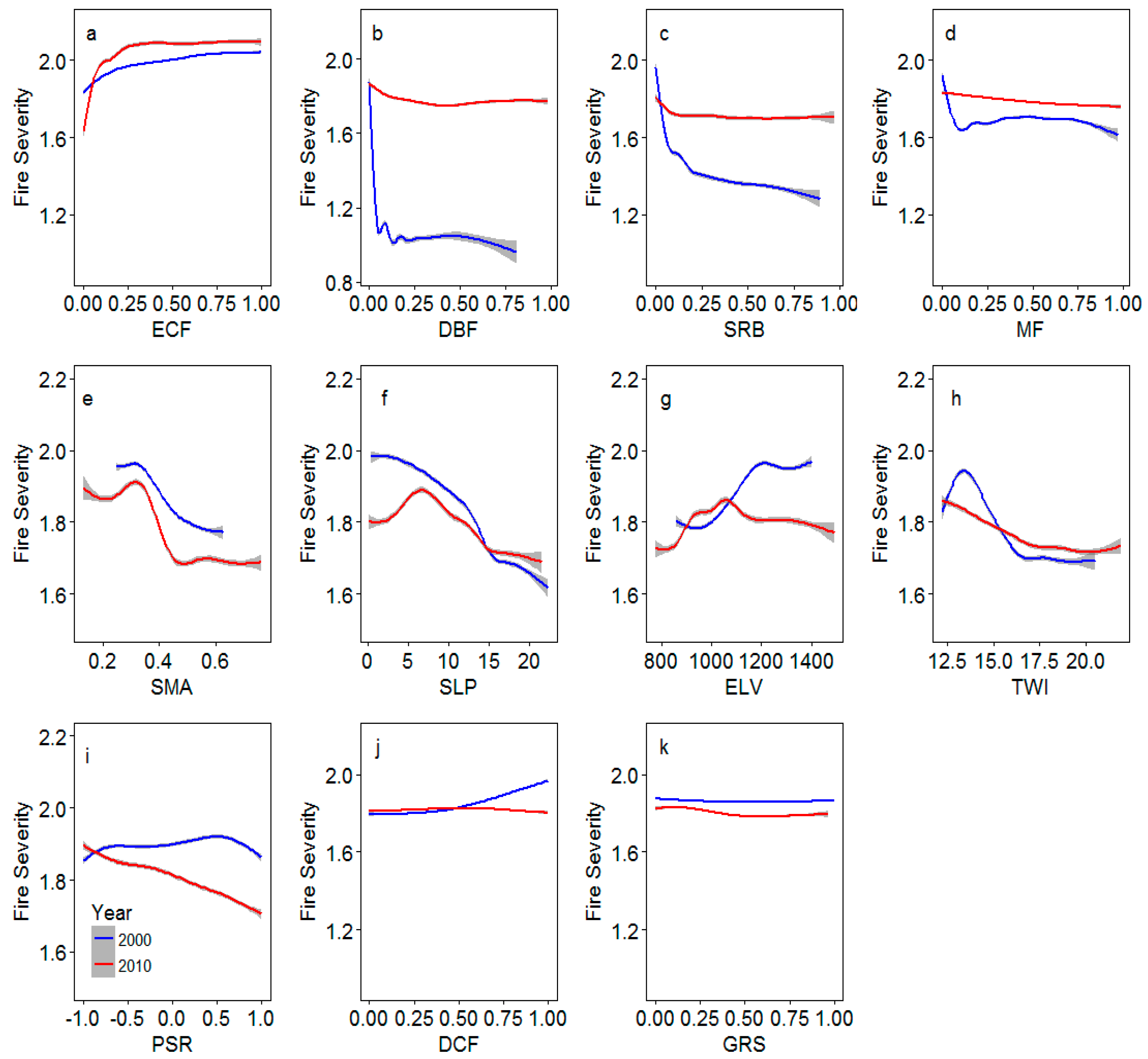
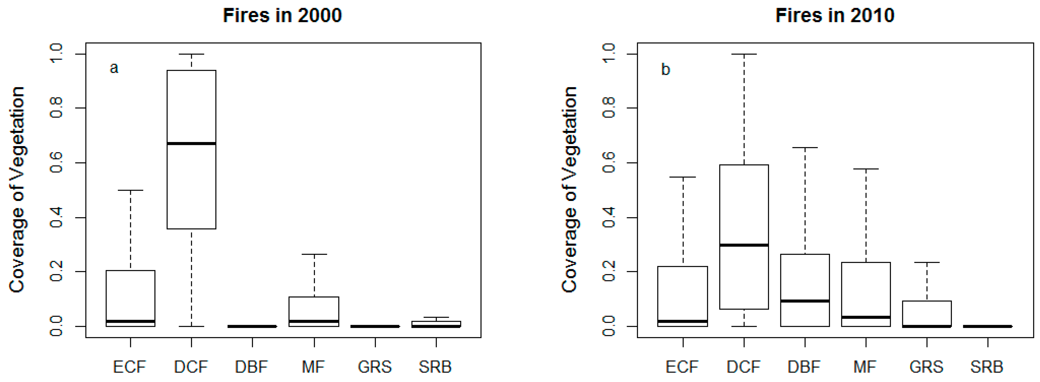
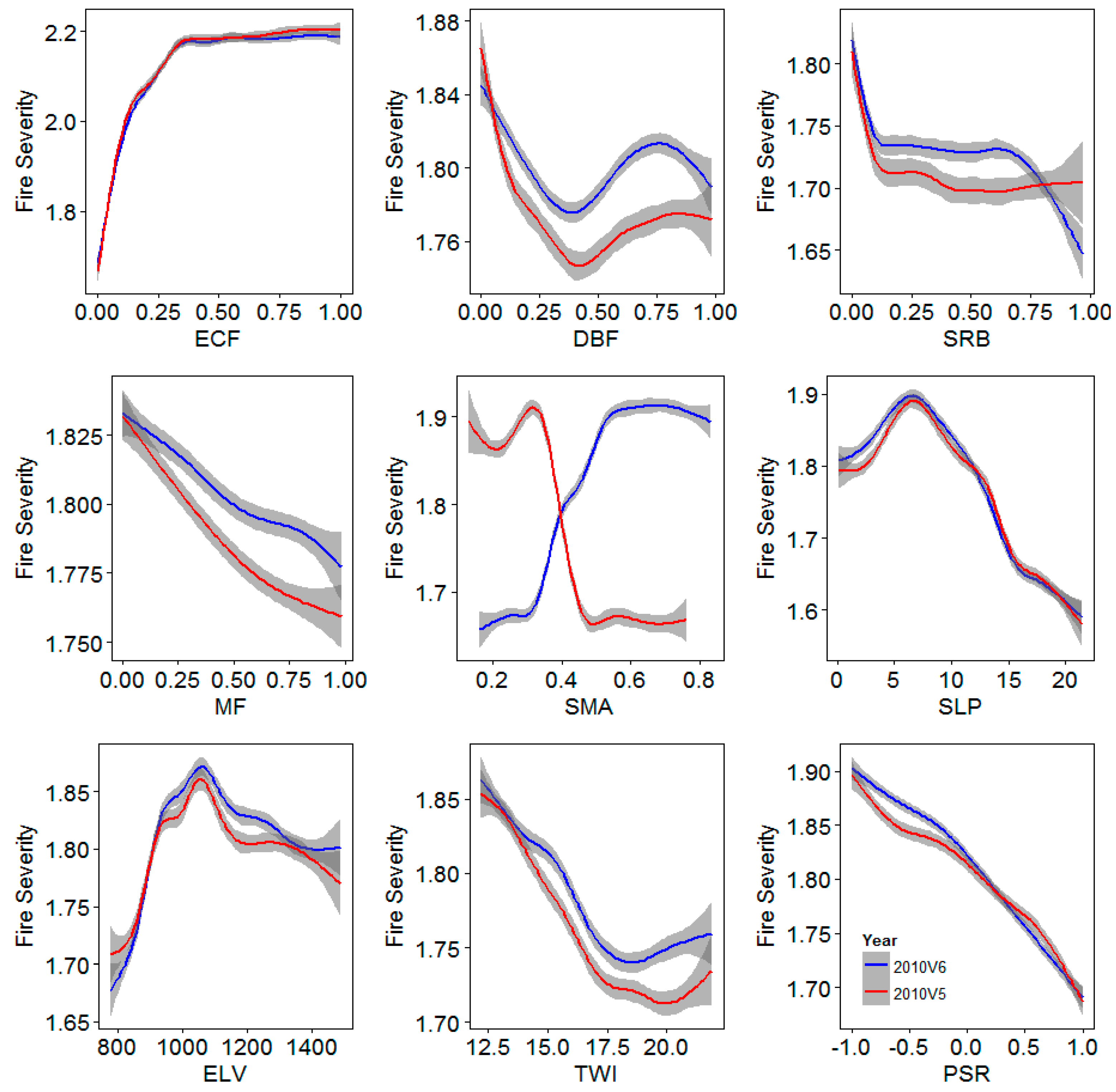
3.3. Relationships between Environmental Variables and Fire Severity
4. Discussion
4.1. Environmental Influences on Fire Severity
4.2. Prediction of Fire Severity
4.3. Limitation and Uncertainty
5. Conclusions
Acknowledgments
Author Contributions
Conflicts of Interest
Appendix A


Appendix B

| Variables | Moran’s I of Fires 2000 | Moran’s I of Fires 2010 |
|---|---|---|
| Fire Severity | 0.132 | 0.078 |
| SMA_V5 | 0.224 | 0.124 |
| ELV | 0.192 | 0.236 |
| PSR | 0.061 | 0.066 |
| SLP | 0.120 | 0.075 |
| TWI | 0.054 | 0.06 |
| ECF | 0.078 | 0.092 |
| DCF | 0.178 | 0.107 |
| DBF | 0.041 | 0.19 |
| MF | 0.134 | 0.07 |
| GRS | 0.104 | 0.056 |
| SRB | 0.035 | 0.156 |
References
- De Groot, W.J.; Flannigan, M.D.; Cantin, A.S. Climate change impacts on future boreal fire regimes. For. Ecol. Manag. 2013, 294, 35–44. [Google Scholar] [CrossRef]
- Flannigan, M.; Stocks, B.; Turetsky, M.; Wotton, M. Impacts of climate change on fire activity and fire management in the circumboreal forest. Glob. Chang. Biol. 2009, 15, 549–560. [Google Scholar] [CrossRef]
- Stephens, S.L.; Burrows, N.; Buyantuyev, A.; Gray, R.W.; Keane, R.E.; Kubian, R.; Liu, S.; Seijo, F.; Shu, L.; Tolhurst, K.G.; et al. Temperate and boreal forest mega-fires: Characteristics and challenges. Front. Ecol. Environ. 2014, 12, 115–122. [Google Scholar] [CrossRef]
- Conard, S.G.; Solomon, A.M. Effects of wildland fire on regional and global carbon stocks in a changing environment. Dev. Environ. Sci. 2008, 8, 109–138. [Google Scholar]
- Harden, J.; Trumbore, S.; Stocks, B.; Hirsch, A.; Gower, S.; O’neill, K.; Kasischke, E. The role of fire in the boreal carbon budget. Glob. Chang. Biol. 2000, 6, 174–184. [Google Scholar] [CrossRef]
- Bond-Lamberty, B.; Peckham, S.D.; Gower, S.T.; Ewers, B.E. Effects of fire on regional evapotranspiration in the central Canadian boreal forest. Glob. Chang. Biol. 2009, 15, 1242–1254. [Google Scholar] [CrossRef]
- Jin, Y.; Roy, D. Fire-induced albedo change and its radiative forcing at the surface in northern Australia. Geophys. Res. Lett. 2005, 32. [Google Scholar] [CrossRef]
- Keane, R.E.; Agee, J.K.; Fulé, P.; Keeley, J.E.; Key, C.; Kitchen, S.G.; Miller, R.; Schulte, L.A. Ecological effects of large fires on US landscapes: Benefit or catastrophe? Int. J. Wildland Fire 2008, 17, 696–712. [Google Scholar] [CrossRef]
- Anderson-Teixeira, K.J.; Miller, A.D.; Mohan, J.E.; Hudiburg, T.W.; Duval, B.D.; Delucia, E.H. Altered dynamics of forest recovery under a changing climate. Glob. Chang. Biol. 2013, 19, 2001–2021. [Google Scholar] [CrossRef] [PubMed]
- Bond, W.J.; Keeley, J.E. Fire as a global ‘herbivore’: The ecology and evolution of flammable ecosystems. Trends Ecol. Evol. 2005, 20, 387–394. [Google Scholar] [CrossRef] [PubMed]
- Johnstone, J.F.; Hollingsworth, T.N.; Chapin, F.S.; Mack, M.C. Changes in fire regime break the legacy lock on successional trajectories in Alaskan boreal forest. Glob. Chang. Biol. 2010, 16, 1281–1295. [Google Scholar] [CrossRef]
- Turner, M.G.; Hargrove, W.W.; Gardner, R.H.; Romme, W.H. Effects of fire on landscape heterogeneity in Yellowstone National Park, Wyoming. J. Veg. Sci. 1994, 5, 731–742. [Google Scholar] [CrossRef]
- Amiro, B.; Orchansky, A.; Barr, A.; Black, T.; Chambers, S.; Chapin, F., III; Goulden, M.; Litvak, M.; Liu, H.; McCaughey, J. The effect of post-fire stand age on the boreal forest energy balance. Agric. For. Meteorol. 2006, 140, 41–50. [Google Scholar] [CrossRef]
- Beck, P.S.; Goetz, S.J.; Mack, M.C.; Alexander, H.D.; Jin, Y.; Randerson, J.T.; Loranty, M. The impacts and implications of an intensifying fire regime on Alaskan boreal forest composition and albedo. Glob. Chang. Biol. 2011, 17, 2853–2866. [Google Scholar] [CrossRef]
- Rogers, B.M.; Soja, A.J.; Goulden, M.L.; Randerson, J.T. Influence of tree species on continental differences in boreal fires and climate feedbacks. Nat. Geosci. 2015, 8, 228–234. [Google Scholar] [CrossRef]
- De Groot, W.J.; Cantin, A.S.; Flannigan, M.D.; Soja, A.J.; Gowman, L.M.; Newbery, A. A comparison of Canadian and Russian boreal forest fire regimes. For. Ecol. Manag. 2013, 294, 23–34. [Google Scholar] [CrossRef]
- Running, S.W. Is global warming causing more, larger wildfires? Science 2006, 313, 927–928. [Google Scholar] [CrossRef] [PubMed]
- Van Mantgem, P.J.; Nesmith, J.C.; Keifer, M.; Knapp, E.E.; Flint, A.; Flint, L. Climatic stress increases forest fire severity across the western United States. Ecol. Lett. 2013, 16, 1151–1156. [Google Scholar] [CrossRef] [PubMed]
- Key, C.H.; Benson, N.C. Landscape Assessment (LA). Firemon: Fire Effects Monitoring and Inventory System; U.S. Department of Agriculture, Forest Service, Rocky Mountain Research Station: Fort Collins, CO, USA, 2006. [Google Scholar]
- Lentile, L.B.; Holden, Z.A.; Smith, A.M.S.; Falkowski, M.J.; Hudak, A.T.; Morgan, P.; Lewis, S.A.; Gessler, P.E.; Benson, N.C. Remote sensing techniques to assess active fire characteristics and post-fire effects. Int. J. Wildland Fire 2006, 15, 319–345. [Google Scholar] [CrossRef]
- De Santis, A.; Chuvieco, E. Geocbi: A modified version of the composite burn index for the initial assessment of the short-term burn severity from remotely sensed data. Remote Sens. Environ. 2009, 113, 554–562. [Google Scholar] [CrossRef]
- French, N.H.F.; Kasischke, E.S.; Hall, R.J.; Murphy, K.A.; Verbyla, D.L.; Hoy, E.E.; Allen, J.L. Using landsat data to assess fire and burn severity in the north American boreal forest region: An overview and summary of results. Int. J. Wildland Fire 2008, 17, 443–462. [Google Scholar] [CrossRef]
- Hollingsworth, T.N.; Johnstone, J.F.; Bernhardt, E.L.; Chapin, F.S. Fire severity filters regeneration traits to shape community assembly in Alaska’s boreal forest. PLoS ONE 2013, 8, e56033. [Google Scholar] [CrossRef] [PubMed]
- Liu, Z.; Yang, J. Quantifying ecological drivers of ecosystem productivity of the early-successional boreal Larix gmelinii forest. Ecosphere 2014, 5, 1–16. [Google Scholar] [CrossRef]
- Turner, M.G. Disturbance and landscape dynamics in a changing world. Ecology 2010, 91, 2833–2849. [Google Scholar] [CrossRef] [PubMed]
- Rollins, M.G.; Keane, R.E.; Parsons, R.A. Mapping fuels and fire regimes using remote sensing, ecosystem simulation, and gradient modeling. Ecol. Appl. 2004, 14, 75–95. [Google Scholar] [CrossRef]
- Morgan, P.; Keane, R.E.; Dillon, G.K.; Jain, T.B.; Hudak, A.T.; Karau, E.C.; Sikkink, P.G.; Holden, Z.A.; Strand, E.K. Challenges of assessing fire and burn severity using field measures, remote sensing and modelling. Int. J. Wildland Fire 2014, 23, 1045–1460. [Google Scholar] [CrossRef]
- Fang, L.; Yang, J. Atmospheric effects on the performance and threshold extrapolation of multi-temporal landsat derived dNBR for burn severity assessment. Int. J. Appl. Earth Obs. Geoinf. 2014, 33, 10–20. [Google Scholar] [CrossRef]
- Keane, R.E.; Drury, S.A.; Karau, E.C.; Hessburg, P.F.; Reynolds, K.M. A method for mapping fire hazard and risk across multiple scales and its application in fire management. Ecol. Model. 2010, 221, 2–18. [Google Scholar] [CrossRef]
- Stephens, S.L.; Moghaddas, J.J.; Edminster, C.; Fiedler, C.E.; Haase, S.; Harrington, M.; Keeley, J.E.; Knapp, E.E.; McIver, J.D.; Metlen, K.; et al. Fire treatment effects on vegetation structure, fuels, and potential fire severity in western U.S. Forests. Ecol. Appl. 2009, 19, 305–320. [Google Scholar] [CrossRef] [PubMed]
- Whitlock, C.; Higuera, P.E.; McWethy, D.B.; Briles, C.E. Paleoecological perspectives on fire ecology: Revisiting the fire-regime concept. Open Ecol. J. 2010, 3, 6–23. [Google Scholar] [CrossRef]
- Whelan, R.J. The Ecology of Fire; Cambridge University Press: Cambridge, UK, 1995. [Google Scholar]
- Cary, G.J.; Keane, R.E.; Gardner, R.H.; Lavorel, S.; Flannigan, M.D.; Davies, I.D.; Li, C.; Lenihan, J.M.; Rupp, T.S.; Mouillot, F. Comparison of the sensitivity of landscape-fire-succession models to variation in terrain, fuel pattern, climate and weather. Landsc. Ecol. 2006, 21, 121–137. [Google Scholar] [CrossRef]
- Karau, E.C.; Keane, R.E. Burn severity mapping using simulation modelling and satellite imagery. Int. J. Wildland Fire 2010, 19, 710–724. [Google Scholar] [CrossRef]
- Keane, R.E.; Cary, G.J.; Davies, I.D.; Flannigan, M.D.; Gardner, R.H.; Lavorel, S.; Lenihan, J.M.; Li, C.; Rupp, T.S. A classification of landscape fire succession models: Spatial simulations of fire and vegetation dynamics. Ecol. Model. 2004, 179, 3–27. [Google Scholar] [CrossRef]
- Kane, V.R.; Cansler, C.A.; Povak, N.A.; Kane, J.T.; McGaughey, R.J.; Lutz, J.A.; Churchill, D.J.; North, M.P. Mixed severity fire effects within the rim fire: Relative importance of local climate, fire weather, topography, and forest structure. For. Ecol. Manag. 2015, 358, 62–79. [Google Scholar] [CrossRef]
- Birch, D.S.; Morgan, P.; Kolden, C.A.; Abatzoglou, J.T.; Dillon, G.K.; Hudak, A.T.; Smith, A.M.S. Vegetation, topography and daily weather influenced burn severity in central Idaho and western Montana forests. Ecosphere 2015, 6, 1–23. [Google Scholar] [CrossRef]
- Estes, B.L.; Knapp, E.E.; Skinner, C.N.; Miller, J.D.; Preisler, H.K. Factors influencing fire severity under moderate burning conditions in the Klamath Mountains, northern California, USA. Ecosphere 2017, 8. [Google Scholar] [CrossRef]
- Alexander, J.D.; Seavy, N.E.; Ralph, C.J.; Hogoboom, B. Vegetation and topographical correlates of fire severity from two fires in the Klamath-Siskiyou region of Oregon and California. Int. J. Wildland Fire 2006, 15, 237–245. [Google Scholar] [CrossRef]
- Lentile, L.B.; Smith, F.W.; Shepperd, W.D. Influence of topography and forest structure on patterns of mixed severity fire in ponderosa pine forests of the South Dakota Black Hills, USA. Int. J. Wildland Fire 2006, 15, 557–566. [Google Scholar] [CrossRef]
- Peters, D.P.; Pielke, R.A., Sr.; Bestelmeyer, B.T.; Allen, C.D.; Munson-McGee, S.; Havstad, K.M. Cross-scale interactions, nonlinearities, and forecasting catastrophic events. Proc. Natl. Acad. Sci. USA 2004, 101, 15130–15135. [Google Scholar] [CrossRef] [PubMed]
- Dillon, G.K.; Holden, Z.A.; Morgan, P.; Crimmins, M.A.; Heyerdahl, E.K.; Luce, C.H. Both topography and climate affected forest and woodland burn severity in two regions of the western US, 1984 to 2006. Ecosphere 2011, 2, 1–33. [Google Scholar] [CrossRef]
- Fang, L.; Yang, J.; Zu, J.; Li, G.; Zhang, J. Quantifying influences and relative importance of fire weather, topography, and vegetation on fire size and fire severity in a Chinese boreal forest landscape. For. Ecol. Manag. 2015, 356, 2–12. [Google Scholar] [CrossRef]
- Parks, S.A.; Parisien, M.A.; Miller, C.; Dobrowski, S.Z. Fire activity and severity in the western US vary along proxy gradients representing fuel amount and fuel moisture. PLoS ONE 2014, 9, e99699. [Google Scholar] [CrossRef] [PubMed]
- Viedma, O.; Quesada, J.; Torres, I.; De Santis, A.; Moreno, J.M. Fire severity in a large fire in a pinus pinaster forest is highly predictable from burning conditions, stand structure, and topography. Ecosystems 2014, 18, 237–250. [Google Scholar] [CrossRef]
- Cansler, C.A.; McKenzie, D. Climate, fire size, and biophysical setting control fire severity and spatial pattern in the northern Cascade Range, USA. Ecol. Appl. 2014, 24, 1037–1056. [Google Scholar] [CrossRef] [PubMed]
- Clarke, P.J.; Knox, K.J.E.; Bradstock, R.A.; Munoz-Robles, C.; Kumar, L.; Ward, D. Vegetation, terrain and fire history shape the impact of extreme weather on fire severity and ecosystem response. J. Veg. Sci. 2014, 25, 1033–1044. [Google Scholar] [CrossRef]
- Qi, Y.; Dennison, P.E.; Spencer, J.; Riano, D. Monitoring live fuel moisture using soil moisture and remote sensing proxies. Fire Ecol. 2012, 8, 71–87. [Google Scholar]
- Yebra, M.; Dennison, P.E.; Chuvieco, E.; Riaño, D.; Zylstra, P.; Hunt, E.R.; Danson, F.M.; Qi, Y.; Jurdao, S. A global review of remote sensing of live fuel moisture content for fire danger assessment: Moving towards operational products. Remote Sens. Environ. 2013, 136, 455–468. [Google Scholar] [CrossRef]
- Barrett, K.; Kasischke, E.; McGuire, A.; Turetsky, M.; Kane, E. Modeling fire severity in black spruce stands in the Alaskan boreal forest using spectral and non-spectral geospatial data. Remote Sens. Environ. 2010, 114, 1494–1503. [Google Scholar] [CrossRef]
- Holden, Z.A.; Morgan, P.; Evans, J.S. A predictive model of burn severity based on 20-year satellite-inferred burn severity data in a large southwestern US wilderness area. For. Ecol. Manag. 2009, 258, 2399–2406. [Google Scholar]
- Kane, V.R.; Lutz, J.A.; Alina Cansler, C.; Povak, N.A.; Churchill, D.J.; Smith, D.F.; Kane, J.T.; North, M.P. Water balance and topography predict fire and forest structure patterns. For. Ecol. Manag. 2015, 338, 1–13. [Google Scholar] [CrossRef]
- Ponomarev, E.; Kharuk, V.; Ranson, K. Wildfires dynamics in siberian larch forests. Forests 2016, 7, 125. [Google Scholar] [CrossRef]
- Fan, Q.; Wang, C.; Zhang, D.; Zang, S. Environmental influences on forest fire regime in the Greater Hinggan Mountains, northeast China. Forests 2017, 8, 372. [Google Scholar] [CrossRef]
- Fang, J.; Chen, A.; Peng, C.; Zhao, S.; Ci, L. Changes in forest biomass carbon storage in China between 1949 and 1998. Science 2001, 292, 2320–2322. [Google Scholar] [CrossRef] [PubMed]
- Liu, Z.; Yang, J.; Chang, Y.; Weisberg, P.J.; He, H.S. Spatial patterns and drivers of fire occurrence and its future trend under climate change in a boreal forest of northeast China. Glob. Chang. Biol. 2012, 18, 2041–2056. [Google Scholar] [CrossRef]
- Wang, C.; Gower, S.T.; Wang, Y.; Zhao, H.; Yan, P.; Lamberty, B.P. The influence of fire on carbon distribution and net primary production of boreal larix gmelinii forests in north-eastern China. Glob. Chang. Biol. 2001, 7, 719–730. [Google Scholar] [CrossRef]
- Liu, Z.; Yang, J.; He, H.S. Identifying the threshold of dominant controls on fire spread in a boreal forest landscape of northeast China. PLoS ONE 2013, 8, e55618. [Google Scholar] [CrossRef] [PubMed]
- Cai, W.; Yang, J.; Liu, Z.; Hu, Y.; Weisberg, P.J. Post-fire tree recruitment of a boreal larch forest in northeast China. For. Ecol. Manag. 2013, 307, 20–29. [Google Scholar] [CrossRef]
- Kong, J.; Yang, J.; Chu, H.; Xiang, X. Effects of wildfire and topography on soil nitrogen availability in a boreal larch forest of northeastern China. Int. J. Wildland Fire 2015, 24, 433–442. [Google Scholar] [CrossRef]
- Chander, G.; Markham, B.L.; Helder, D.L. Summary of current radiometric calibration coefficients for landsat MSS, TM, ETM+, and EO-1 ALI sensors. Remote Sens. Environ. 2009, 113, 893–903. [Google Scholar] [CrossRef]
- Vermote, E.F.; Tanre, D.; Deuze, J.L.; Herman, M.; Morcette, J.J. Second simulation of the satellite signal in the solar spectrum, 6S: An overview. IEEE Trans. Geosci. Remote Sens. 1997, 35, 675–686. [Google Scholar] [CrossRef]
- Canty, M.J.; Nielsen, A.A. Automatic radiometric normalization of multitemporal satellite imagery with the iteratively re-weighted mad transformation. Remote Sens. Environ. 2008, 112, 1025–1036. [Google Scholar] [CrossRef]
- Mu, Q.; Zhao, M.; Running, S.W. Improvements to a modis global terrestrial evapotranspiration algorithm. Remote Sens. Environ. 2011, 115, 1781–1800. [Google Scholar] [CrossRef]
- Kim, H.W.; Hwang, K.; Mu, Q.; Lee, S.O.; Choi, M. Validation of modis 16 global terrestrial evapotranspiration products in various climates and land cover types in Asia. KSCE J. Civ. Eng. 2012, 16, 229–238. [Google Scholar] [CrossRef]
- Wang, L.; Hunt, E.R.; Qu, J.J.; Hao, X.; Daughtry, C.S.T. Remote sensing of fuel moisture content from ratios of narrow-band vegetation water and dry-matter indices. Remote Sens. Environ. 2013, 129, 103–110. [Google Scholar] [CrossRef]
- Running, S.W.; Mu, Q.; Zhao, M.; Moreno, A. Modis Global Terrestrial Evapotranspiration (ET) Product (NASA MOD16A2/A3) NASA Earth Observing System Modis Land Algorithm; NASA: Washington, DC, USA, 2017.
- Masek, J.G.; Huang, C.; Wolfe, R.; Cohen, W.; Hall, F.; Kutler, J.; Nelson, P. North American forest disturbance mapped from a decadal landsat record. Remote Sens. Environ. 2008, 112, 2914–2926. [Google Scholar] [CrossRef]
- Friedl, M.A.; Brodley, C.E. Decision tree classification of land cover from remotely sensed data. Remote Sens. Environ. 1997, 61, 399–409. [Google Scholar] [CrossRef]
- Yang, J.; He, H.S.; Shifley, S.R.; Gustafson, E.J. Spatial patterns of modern period human-caused fire occurrence in the Missouri Ozark Highlands. For. Sci. 2007, 53, 1–15. [Google Scholar]
- Quinn, P.; Beven, K. Spatial and temporal predictions of soil moisture dynamics, runoff, variable source areas and evapotranspiration for Plynlimon, Mid-Wales. Hydrol. Process. 1993, 7, 425–448. [Google Scholar] [CrossRef]
- Sörensen, R.; Zinko, U.; Seibert, J. On the calculation of the topographic wetness index: Evaluation of different methods based on field observations. Hydrol. Earth Syst. Sci. Discuss. 2006, 10, 101–112. [Google Scholar] [CrossRef]
- Qin, C.; Zhu, A.; Yang, L.; Li, B.; Pei, T. Topographic wetness index computed using multiple flow direction algorithm and local maximum downslope gradient. In Proceedings of the 7th International Workshop of Geographical Information System, Beijing, China, 12–14 September 2007. [Google Scholar]
- Wotton, B.M. Interpreting and using outputs from the Canadian forest fire danger rating system in research applications. Environ. Ecol. Stat. 2009, 16, 107–131. [Google Scholar] [CrossRef]
- Keane, R.E. Wildland Fuel Fundamentals and Applications; Springer: Berlin, Germany, 2015. [Google Scholar]
- Carlson, T.N. Regional-scale estimates of surface moisture availability and thermal inertia using remote thermal measurements. Remote Sens. Rev. 1986, 1, 197–247. [Google Scholar] [CrossRef]
- Ha, W.; Gowda, P.H.; Howell, T.A. A review of downscaling methods for remote sensing-based irrigation management: Part I. Irrig. Sci. 2012, 31, 831–850. [Google Scholar] [CrossRef]
- De’ath, G. Boosted trees for ecological modeling and prediction. Ecology 2007, 88, 243–251. [Google Scholar] [CrossRef]
- Elith, J.; Leathwick, J.R.; Hastie, T. A working guide to boosted regression trees. J. Anim. Ecol. 2008, 77, 802–813. [Google Scholar] [CrossRef] [PubMed]
- Paradis, E.; Claude, J.; Strimmer, K. Ape: Analyses of phylogenetics and evolution in R language. Bioinformatics 2004, 20, 289–290. [Google Scholar] [CrossRef] [PubMed]
- Legendre, P. Spatial autocorrelation: Trouble or new paradigm? Ecology 1993, 74, 1659–1673. [Google Scholar] [CrossRef]
- Ferster, C.; Eskelson, B.; Andison, D.; LeMay, V. Vegetation Mortality within Natural Wildfire Events in the Western Canadian Boreal Forest: What Burns and Why? Forests 2016, 7, 187. [Google Scholar] [CrossRef]
- Whitman, E.; Parisien, M.-A.; Thompson, D.; Hall, R.; Skakun, R.; Flannigan, M. Variability and drivers of burn severity in the northwestern Canadian boreal forest. Ecosphere 2018, 9, e02128. [Google Scholar] [CrossRef]
- Bigler, C.; Kulakowski, D.; Veblen, T.T. Multiple disturbance interactions and drought influence fire severity in Rocky Mountain subalpine forests. Ecology 2005, 86, 3018–3029. [Google Scholar] [CrossRef]
- Schoennagel, T.; Veblen, T.T.; Romme, W.H. The interaction of fire, fuels, and climate across Rocky Mountain forests. BioScience 2004, 54, 661–676. [Google Scholar] [CrossRef]
- Rupp, T.S.; Starfield, A.M.; Chapin, F.S.; Duffy, P. Modeling the impact of black spruce on the fire regime of Alaskan boreal forest. Clim. Chang. 2002, 55, 213–233. [Google Scholar] [CrossRef]
- Johnstone, J.F.; Rupp, T.S.; Olson, M.; Verbyla, D. Modeling impacts of fire severity on successional trajectories and future fire behavior in Alaskan boreal forests. Landsc. Ecol. 2011, 26, 487–500. [Google Scholar] [CrossRef]
- Kobayashi, M.; Yury, P.N.; Olga, A.Z.; Takuya, K.; Yojiro, M.; Toshiya, Y.; Fuyuki, S.; Kaichiro, S.; Takayoshi, K. Regeneration after forest fires in mixed conifer broad-leaved forests of the amur region in far eastern Russia: The relationship between species specific traits against fire and recent fire regimes. Eurasian J. For. Res. 2007, 10, 51–58. [Google Scholar]
- Zhao, F.; Shu, L.; Wang, M.; Liu, B.; Yang, L. Influencing factors on early vegetation restoration in burned area of Pinus Pumila—Larch forest. Acta Ecol. Sin. 2012, 32, 57–61. [Google Scholar] [CrossRef]
- Zhao, F.; Shu, L.; Wang, Q.; Wang, M.; Tian, X. Emissions of volatile organic compounds from heated needles and twigs of Pinus Pumila. J. For. Res. 2011, 22, 243–248. [Google Scholar] [CrossRef]
- Ryan, K.C. Dynamic interactions between forest structure and fire behavior in boreal ecosystems. Silva Fenn. 2002, 36, 13–39. [Google Scholar] [CrossRef]
- Kopecký, M.; Čížková, Š. Using topographic wetness index in vegetation ecology: Does the algorithm matter? Appl. Veg. Sci. 2010, 13, 450–459. [Google Scholar] [CrossRef]
- Xiao, J.; Zhuang, Q. Drought effects on large fire activity in Canadian and Alaskan forests. Environ. Res. Lett. 2007, 2, 044003. [Google Scholar] [CrossRef]
- Parks, S.A.; Miller, C.; Nelson, C.R.; Holden, Z.A. Previous fires moderate burn severity of subsequent wildland fires in two large western US wilderness areas. Ecosystems 2014, 17, 29–42. [Google Scholar] [CrossRef]
- Li, X.; He, H.S.; Wu, Z.; Liang, Y.; Schneiderman, J.E. Comparing effects of climate warming, fire, and timber harvesting on a boreal forest landscape in northeastern China. PLoS ONE 2013, 8, e59747. [Google Scholar] [CrossRef] [PubMed]
- Arroyo, L.A.; Pascual, C.; Manzanera, J.A. Fire models and methods to map fuel types: The role of remote sensing. For. Ecol. Manag. 2008, 256, 1239–1252. [Google Scholar] [CrossRef]
- Tian, X.; Mcrae, D.J.; Shu, L.; Wang, M.; Li, H. Satellite remote-sensing technologies used in forest fire management. J. For. Res. 2005, 16, 73–78. [Google Scholar]
- Pierce, A.D.; Farris, C.A.; Taylor, A.H. Use of random forests for modeling and mapping forest canopy fuels for fire behavior analysis in Lassen Volcanic National Park, California, USA. For. Ecol. Manag. 2012, 279, 77–89. [Google Scholar] [CrossRef]
- Song, C. Optical remote sensing of forest leaf area index and biomass. Prog. Phys. Geogr. 2012, 37, 98–113. [Google Scholar] [CrossRef]
- Keane, R.E.; Burgan, R.; van Wagtendonk, J. Mapping wildland fuels for fire management across multiple scales: Integrating remote sensing, GIS, and biophysical modeling. Int. J. Wildland Fire 2001, 10, 301–319. [Google Scholar] [CrossRef]
- Cyr, D.; Gauthier, S.; Bergeron, Y. Scale-dependent determinants of heterogeneity in fire frequency in a coniferous boreal forest of eastern Canada. Landsc. Ecol. 2007, 22, 1325–1339. [Google Scholar] [CrossRef]
- Parisien, M.A.; Parks, S.A.; Krawchuk, M.A.; Flannigan, M.D.; Bowman, L.M.; Moritz, M.A. Scale-dependent controls on the area burned in the boreal forest of Canada, 1980–2005. Ecol. Appl. 2011, 21, 789–805. [Google Scholar] [CrossRef] [PubMed]
- Parks, S.A.; Parisien, M.-A.; Miller, C. Multi-scale evaluation of the environmental controls on burn probability in a southern Sierra Nevada landscape. Int. J. Wildland Fire 2011, 20, 815–828. [Google Scholar] [CrossRef]
- Wu, Z.; He, H.S.; Bobryk, C.W.; Liang, Y. Scale effects of vegetation and topography on burn severity under prevailing fire weather conditions in boreal forest landscapes of northeastern China. Scand. J. For. Res. 2014, 29, 60–70. [Google Scholar] [CrossRef]
- Veraverbeke, S.; Sedano, F.; Hook, S.J.; Randerson, J.T.; Jin, Y.; Rogers, B.M. Mapping the daily progression of large wildland fires using modis active fire data. Int. J. Wildland Fire 2014, 23, 655–667. [Google Scholar] [CrossRef]
- Parks, S.A. Mapping day-of-burning with coarse-resolution satellite fire-detection data. Int. J. Wildland Fire 2014, 23, 215–223. [Google Scholar] [CrossRef]


| Occurrence Date | DOY † | Duration (Day) | Longitude | Latitude | Burned Area (ha) |
|---|---|---|---|---|---|
| 17 June 2000 | 168 | 7 | 122.830 | 51.891 | 8518.5 |
| 17 June 2000 | 168 | 5 | 123.175 | 51.314 | 2918.3 |
| 18 June 2000 | 169 | 3 | 123.294 | 51.724 | 1443.6 |
| 12 June 2010 | 163 | 1 | 123.092 | 52.003 | 207.4 |
| 12 June 2010 | 163 | 1 | 122.947 | 51.420 | 320.1 |
| 13 June 2010 | 164 | 1 | 122.844 | 52.036 | 394.8 |
| 15 June 2010 | 166 | 1 | 122.821 | 51.813 | 26.3 |
| 15 June 2010 | 166 | 1 | 123.579 | 51.583 | 29.0 |
| 15 June 2010 | 166 | 1 | 123.587 | 51.559 | 104.5 |
| 20 June 2010 | 171 | 1 | 122.908 | 52.027 | 47.0 |
| 25 June 2010 | 176 | 1 | 123.513 | 51.577 | 17.4 |
| 26 June 2010 | 177 | 5 | 123.486 | 51.305 | 2891.5 |
| 26 June 2010 | 177 | 5 | 123.252 | 51.472 | 1926.1 |
| 27 June 2010 | 178 | 1 | 123.116 | 51.300 | 102.4 |
| 27 June 2010 | 178 | 3 | 123.182 | 51.431 | 255.1 |
| 27 June 2010 | 178 | 3 | 123.224 | 51.390 | 734.6 |
| 27 June 2010 | 178 | 3 | 123.108 | 51.435 | 258.8 |
| 28 June 2010 | 179 | 1 | 123.302 | 51.450 | 260.4 |
| 28 June 2010 | 179 | 1 | 122.784 | 51.459 | 536.0 |
| 28 June 2010 | 179 | 3 | 123.065 | 51.391 | 984.3 |
| 29 June 2010 | 180 | 1 | 122.922 | 51.879 | 670.8 |
| Category | Variable | Description | Mean ± SD (2000 & 2010) |
|---|---|---|---|
| Vegetation † | ECF | Percentage of Landsat pixels classified into evergreen coniferous trees within 240 m burned pixels, were primarily Pinus pumila shrublands and Larix gmelinii-Pinus pumila forest. | 0.158 ± 0.261 0.169 ± 0.278 |
| DCF | Percentage of larch forest. The three dominant larch forests are Larix gmelinii-Ledum palustre L., Larix gmelinii-grass, and Larix gmelinii-Rhododendron dahurica L. | 0.615 ± 0.324 0.350 ± 0.302 | |
| DBF | Percentage of broad leaf forest. The white birch and aspen are dominant broad leaf species. | 0.017 ± 0.057 0.177 ± 0.218 | |
| MF | Percentage of mixed forest. Composited by broad leaf trees and coniferous trees. | 0.086 ± 0.145 0.150 ± 0.218 | |
| GRS | Percentage of grassland. | 0.047 ± 0.135 0.086 ± 0.166 | |
| SRB | Percentage of shrublands, typically distributed in open land along the river and disturbed areas. | 0.035 ± 0.097 0.041 ± 0.134 | |
| Topography | ELV | Elevation (meters) derived from the aggregated ASTER GDEM at 240 m spatial resolution. | 1089 ± 92.862 1017 ± 107.316 |
| PSR | Potential solar radiation. It ranges from −1 to 1, where high values represent xeric exposures. | −0.024 ± 0.715 −0.173 ± 0.683 | |
| SLP | Slope (degree) computed from aggregated DEM. | 8.840 ± 4.090 8.958 ± 3.992 | |
| TWI | Topographic wetness index (unitless) is computed from the slope and the upslope contributing area per unit contour length. | 13.953 ± 1.313 14.024 ± 1.528 | |
| Surface moisture | SMA | SMA is calculated from MOD16A2 and represents land surface moisture availability. The higher SMA value indicates the wetter land surface. | 0.494 ± 0.099 0.411 ± 0.153 |
| Predicted Severity of 2000 | Predicted Severity of 2010 | |||||||
|---|---|---|---|---|---|---|---|---|
| Severity Class | Low | Moderate | High | Producer’s Accuracy | Low | Moderate | High | Producer’s Accuracy |
| Low | 50 | 26 | 7 | 60.2% | 196 | 263 | 94 | 35.4% |
| Moderate | 261 | 496 | 142 | 55.2% | 95 | 276 | 115 | 56.8% |
| High | 42 | 369 | 1184 | 74.2% | 33 | 431 | 662 | 58.8% |
| User’s Accuracy | 14.2% | 55.7% | 88.8% | - | 60.5% | 28.5% | 76.0% | - |
| Overall Accuracy | 67.1% | 52.4% | ||||||
© 2018 by the authors. Licensee MDPI, Basel, Switzerland. This article is an open access article distributed under the terms and conditions of the Creative Commons Attribution (CC BY) license (http://creativecommons.org/licenses/by/4.0/).
Share and Cite
Fang, L.; Yang, J.; White, M.; Liu, Z. Predicting Potential Fire Severity Using Vegetation, Topography and Surface Moisture Availability in a Eurasian Boreal Forest Landscape. Forests 2018, 9, 130. https://doi.org/10.3390/f9030130
Fang L, Yang J, White M, Liu Z. Predicting Potential Fire Severity Using Vegetation, Topography and Surface Moisture Availability in a Eurasian Boreal Forest Landscape. Forests. 2018; 9(3):130. https://doi.org/10.3390/f9030130
Chicago/Turabian StyleFang, Lei, Jian Yang, Megan White, and Zhihua Liu. 2018. "Predicting Potential Fire Severity Using Vegetation, Topography and Surface Moisture Availability in a Eurasian Boreal Forest Landscape" Forests 9, no. 3: 130. https://doi.org/10.3390/f9030130
APA StyleFang, L., Yang, J., White, M., & Liu, Z. (2018). Predicting Potential Fire Severity Using Vegetation, Topography and Surface Moisture Availability in a Eurasian Boreal Forest Landscape. Forests, 9(3), 130. https://doi.org/10.3390/f9030130