Enhancing the Estimation of Stem-Size Distributions for Unimodal and Bimodal Stands in a Boreal Mixedwood Forest with Airborne Laser Scanning Data

Abstract

Stem size distribution (SSD), which describes tree frequencies in diameter classes within an area, has a variety of direct and indirect applications that are critical for forest management. In this study, we evaluated which structural characteristics derived from Airborne Laser Scanning (ALS) data were best able to differentiate between unimodal and bimodal stands in a managed boreal mixedwood forest in Alberta, Canada. We then used wall-to-wall ALS data to predict (for 20 m-by-20 m grid cells) the parameters of a Weibull SSD in unimodal cells, and a Finite Mixture Model (FMM) in bimodal cells. The resulting SSDs were evaluated for their fit to ground plot-measured SSDs using an Error Index (EI). We found that the variance of ALS return heights was the best metric for differentiating between unimodal and bimodal stands, with a classification accuracy of 77%. Parameters of both the Weibull and FMM distributions were accurately predicted (r² ~ 0.5, Root Mean Square Error (RMSE) ~ 30%), and that differentiating for modality prior to estimating SSD improved the accuracy of estimates (EI of 49.13 with differentiation versus 51.31 without differentiation). Unique to our presented approach is the stratification by SSD modality prior to the modelling of distributions. To achieve this, we apply a threshold to an ALS metric that allows SSD modality to be distinguished for each cell at the landscape level, and this a priori information is then used to ensure that the appropriate distribution is modelled. Our approach is parsimonious and efficient, enabling improved accuracy in SSD estimation across diverse landscapes when ALS data is the sole data source.

1. Introduction

Forest professionals manage forests using detailed forest inventories based on measurements and models characterizing tree dimensions, timber volume, and stand composition [1]. A critical component of forest inventories is the stem size distribution (SSD), which represents the relative frequency of tree diameters on a given area (e.g. plot or stand; [2]). SSDs are versatile and are useful for a range of timber production and ecological monitoring purposes. For example, the SSD can be used directly to describe stand attributes such as structure, age, and volume [3,4,5], or used as inputs to models that can describe product quality [6], forecast growth, or provide information for planning and management considerations [7]. To support these information needs, there is increasing interest in the capacity to estimate stand-level SSDs over large areas, and to understand patterns of their variance—particularly across the diverse species and age gradients that exist in mixedwood stands. Mixedwood stands are the most common habitat in the boreal forest, which makes up almost 2 billion hectares globally—28% of which is in Canada, representing 78% of the nation’s total forested area [8].

Currently, SSDs are usually acquired using field measurements where tree diameters are measured on sample plots and classified into diameter classes. The class sizes used can vary depending on the plot size, stand characteristics, or the application; however, 2-cm diameter classes are most frequently used [9]. SSDs of homogenous stands are typically unimodal, while two or more maxima are often observed in heterogeneous stands with more complex structure. Various statistics, such as the bimodality coefficient or Hartigan’s dip statistic [10], can be used to assess multimodality of SSD. However, it can also be characterized using the ecological characteristics of the stand, including if stands are multilayered [11], have high variance in diameters [12], ages [13], or number of species [14], or by more complex metrics such as the ratio of stem density to top height (D/H; [15]). As stands mature, they do not follow a linear pattern of structural development, making the prediction of mature stand structures difficult [16]. Heterogeneity, typically associated with multimodal stands, results from ecological legacies and disturbance histories specific to individual areas [17].

In addition to size class frequencies, SSDs can be summarized using a variety of statistical models or probability density functions (PDFs). The most common PDF for characterizing SSDs is the Weibull distribution because of its flexibility with a limited number (two) of parameters to predict or impute [18]. Fitting PDF parameters to measured diameter at breast height (DBH) values relies on optimization techniques such as maximum likelihood estimation (MLE; [19]). Despite the flexibility of the Weibull distribution, it is limited to the characterization of stands with unimodal SSD [20]. If a SSD of a stand is not unimodal, it should be characterized by a more complex distribution or use a nonparametric estimation method such as a Finite Mixture Model (FMM; [15]) or k-Nearest Neighbors (k-NN) [21].

For complete characterization of forest structure, the SSDs of all stands in the area of interest need to be estimated or measured. SSDs derived from field measurements are spatially constrained, time consuming, and expensive to acquire. Hence, field-based estimates of SSDs alone cannot provide the large-area spatial coverage required in a forest management context. A common inventory approach to address the limitation in spatial coverage is to use air-photo interpretation, which can provide complete spatial coverage of an area. However, this approach is limited to the scale of the aerial photography and the expertise of the interpreter, and as a result it is difficult to provide the detailed tree-level information required for a SSD. Eid et al. [22], for a spruce/pine forest in Norway, determined that photo interpretation provided poorer estimates of stand inventory attributes, such as basal area, height, and number of trees, than estimation by other remote sensing methods. They found, for example, deviations of 20% for photo-interpreted height, compared to deviations of 12% for laser scanning estimates. Inaccurate photo-interpreted estimates were projected to have more than three times the loss in the value of a stand when compared to Airborne Laser Scanning (ALS)-based estimates.

These limitations in spatial coverage and accuracy, coupled with increasing financial pressures and needs for highly detailed data, are resulting in the increased use of active remote sensing technologies for informing forest inventories. ALS has been incorporated into forest inventories because it provides very detailed information on forest structure over large spatial extents [23]. It has been demonstrated [24] that attributes such as dominant height, mean diameter, stem number, basal area, and volume can be adequately estimated using ALS data in combination with a sample of ground plots [25,26]. ALS also has been used to characterize SSDs in unimodal stands requiring relatively simple estimation techniques [27] and in multimodal stands with more complex procedures [21]. However, less has been done to estimate SSDs of boreal mixedwood forests, which can have both simple and irregular distributions in neighboring stands, making them more difficult to predict [14], and estimation of stand modality with ALS has been limited to vertical forest structure (e.g. [28,29]). In the case of forests varying between unimodal and multimodal SSDs, the thresholds for applying different fitting techniques is also poorly understood. Landscape-scale evaluation of modality in predicting SSD in mixedwood stands can provide valuable insights into the complexity of these forests.

In this paper, we evaluate the efficacy of ALS metrics to first differentiate plots with unimodal and multimodal SSDs and then to predict parameters of those distributions. Using both ground plot measurements and ALS estimates of plot structural characteristics (e.g., height or age), we investigate the capacity of ALS metrics to distinguish between areas with single or multimodal distributions and then apply ALS to predict SSDs with the distribution most appropriate to the characterized distribution type. We then compare ALS parameter estimates to fitted parameters and ground measured SSDs. Finally, we discuss the applications of this methodology and explain how estimates could be predicted across an entire area of interest.

2. Materials and Methods

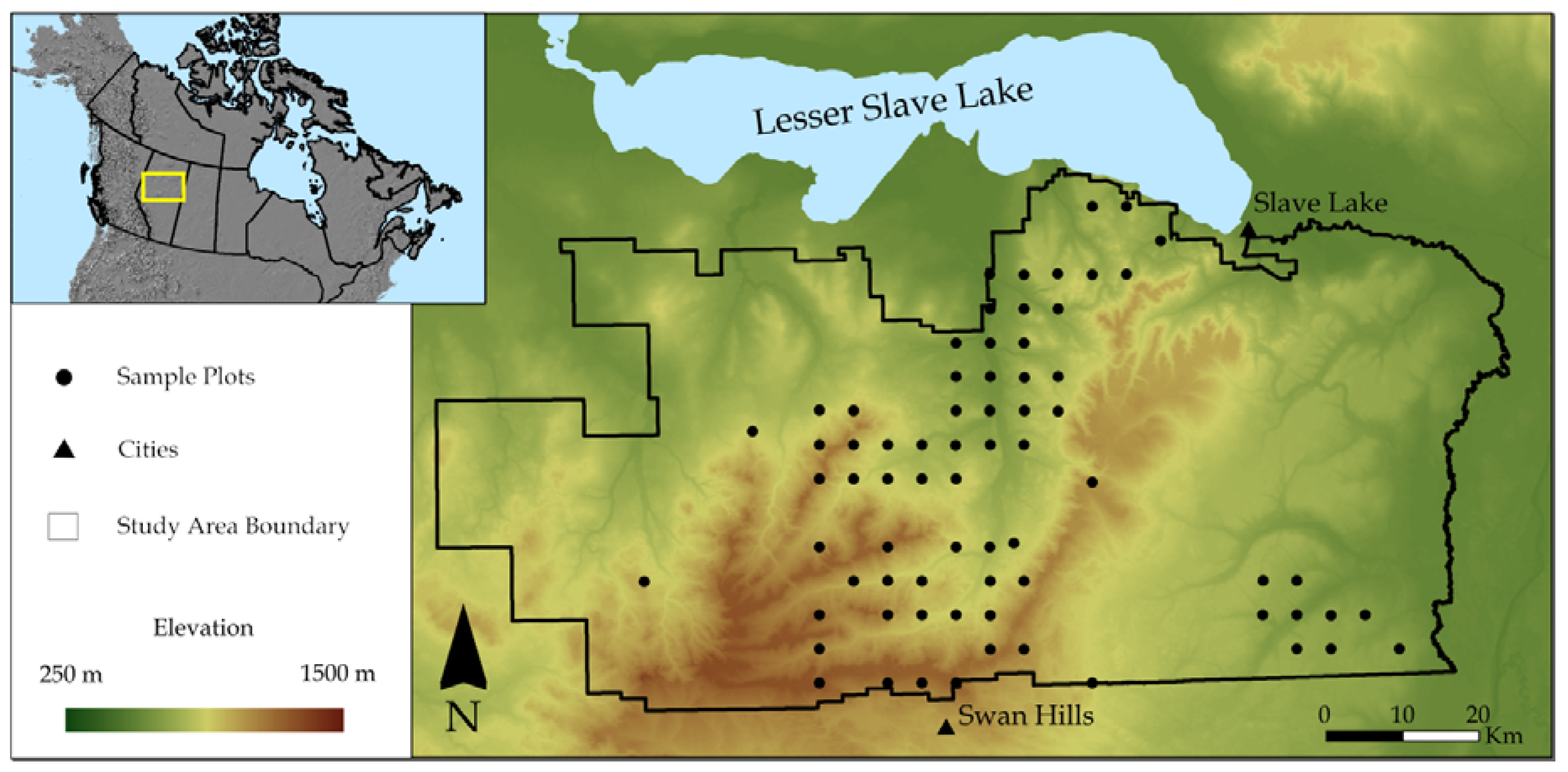
2.1. Study Area

The study area is an actively managed boreal mixedwood forest near Lesser Slave Lake in Alberta, Canada (Figure 1). The area is approximately 700,000 ha in size. Ten tree species were present, with white spruce (Picea glauca), black spruce (Picea mariana), trembling aspen (Populus tremuloides), and lodgepole pine (Pinus contorta) as the most common. The study area covers three natural subregions of Alberta—Central Mixedwood, Lower Foothills, and Upper Foothills. These regions receive approximately 600 mm of annual precipitation and have mean summer and winter temperatures of 20 °C and −21 °C, respectively [30]. Common disturbances include timber harvesting and fires, which are slightly less common than in other forested regions in Alberta. Ecology varies from mesic to wetland areas and features some of the most productive timber-producing areas in Alberta [28].

2.2. Ground Plot Data

The permanent sample plots (PSPs) employed (

Table 1. Summary of plot measurements (n = 71).

Characteristic	Minimum	1st Quartile	Median	3rd Quartile	Maximum	Mean	Std. Deviation
Lorey’s Mean Height (m)	6.13	12.71	15.99	19.83	28.39	16.27	4.97
Quadratic Mean Diameter (cm)	3.88	11.00	13.48	17.08	25.42	14.14	4.72
Age	27.6	53.27	70.19	126.75	197.49	85.34	43.69
Total Volume (m3)	16.99	154.1	248.2	348.8	809.1	280.83	181.96
Density (N/ha)	1075	1875	2650	3138	8325	2644	1194.65

; Figure 1) were a component of the over 650 PSPs established in Alberta since 1960 [31]. The PSPs were established to help understand the stand dynamics in all forest types in Alberta. Measurements included tree height, height to living crown, DBH, species, and crown class for all trees on the plot >7 cm DBH. In addition, cores were taken from trees outside of a sample plot to assess the age structure of the stand. The PSPs are fixed-radius plots with a radius of 11.28 m (400 m²). Measurements in the study area were taken between 2006 and 2007. Only the PSPs that had 20 or more trees (n = 71) were used in the modeling, in order to be effective in predicting parameters for SSD functions that were representative of ground measured SSDs [32].

The bimodality coefficient [33] is a statistical approach to assessing a stand’s modality. It has also been used in botany [34] and psychology [10] and provides a measure from 0 (perfect unimodality) to 1 (perfect bimodality). A critical value of 5/9 (~0.5556) is used to distinguish bimodal (>5/9) from unimodal (<5/9) distributions [10]. We applied the bimodality coefficient to 71 PSPs and identified 23 (32%) as bimodal and 48 as unimodal with respect to SSD.

2.3. ALS Data and Metrics

ALS data were acquired for the study area between 2006 and 2008, with most coverage occurring in 2007. The data were collected with an Optech ALTM 3100 sensor flying at a height of either 1250 m or 1400 m, and scan frequencies of 30 Hz and 33 Hz depending on the year flown (

Table 2. Airborne Laser Scanning (ALS) acquisition characteristics.

Characteristic	Collection Year
	2006	2007–2008
Sensor	Optech ALTM 3100
Flying Height	1250 m	1400 m
Flight Speed	160 kts
Pulse Repetition Frequency	50 kHz	70 kHz
Scan Frequency	30 Hz	33 Hz
Scan Angle	50°
Beam Divergence	0.3 mrad
Average Point Density	1.5 pts/m2

). The result was complete coverage of the study area with an average point density of 1.5 returns/m².

ALS data processing began with separating point clouds into ground and non-ground returns based on adaptive Triangulated Irregular Network (TIN) models [35]. Next, point clouds were normalized to heights above the ground surface before being clipped to the extent of sample plots. Metrics describing the vertical distribution of returns in each plot were calculated based on normalized ALS point clouds using FUSION [36] as well as the statistical software R [37] with the lidR package [38]. A suite of these metrics was selected to fully characterize the height, variability, cover, and structure of the area corresponding to each PSP (

Table 3. ALS metrics used to predict probability density function (PDF) parameters.

Metric	Description	Source	Category
P05	Height of the 5th percentile of returns	McGaughey 2014 [36]	Height
P25	Height of the 25th percentile of returns	McGaughey 2014 [36]	Height
P50	Height of the 50th percentile of returns	McGaughey 2014 [36]	Height
P75	Height of the 75th percentile of returns	McGaughey 2014 [36]	Height
P95	Height of the 95th percentile of returns	McGaughey 2014 [36]	Height
Std. Dev.	Standard deviation of return heights	McGaughey 2014 [36]	Variability of Heights
Variance	Variance of return heights	McGaughey 2014 [36]	Variability of Heights
IQ	Interquartile range of return heights	McGaughey 2014 [36]	Variability of Heights
Skewness	Skewness of return heights	McGaughey 2014 [36]	Variability of Heights
Kurtosis	Kurtosis of return heights	McGaughey 2014 [36]	Variability of Heights
AAD	Average absolute deviation of return heights	McGaughey 2014 [36]	Variability of Heights
Median	Median of return heights	McGaughey 2014 [36]	Variability of Heights
% First Returns Above 2 m	Percent of first returns above 2 meters	McGaughey 2014 [36]	Cover
% All Returns Above 2 m	Percent of all returns above 2 meters	McGaughey 2014 [36]	Cover
0.5 m–2 m Return Proportion	Proportion of returns between 0.5 and 2 m	McGaughey 2014 [36]	Cover
2 m–5 m Return Proportion	Proportion of returns between 2 and 5 m	McGaughey 2014 [36]	Cover
5 m–10 m Return Proportion	Proportion of returns between 5 and 10 m	McGaughey 2014 [36]	Cover
10 m–20 m Return Proportion	Proportion of returns between 10 and 20 m	McGaughey 2014 [36]	Cover
Rumple	Ratio of canopy surface area to plot area	Kane et al. 2010 [39]	Structure
Filling Ratio	Proportion of returns in voxels under the canopy	Tompalski 2012 [40]	Structure
VCI	Vertical complexity index—distribution of abundance of returns in specified height bins	Van Ewijk et al. 2011 [41]	Structure
Vertical Rumple	Measure of variance of vertical structure as a function of filled voxels in point cloud	Tompalski et al. 2015 [42]	Structure
LAD CV	Coefficient of variation of leaf area density—vertical dispersion of foliage density through the canopy	Bouvier et al. 2015 [43]	Structure

). ALS metrics were separated into categories of similar types: height (e.g., height of 50th percentile), cover (e.g., percent above 2 m), variance (e.g., standard deviation), and canopy structure (e.g., rumple).

Filling ratio (FR) is a proportion of filled voxels under the canopy [40]. Voxels are volumetric pixels—cubic bins of a pre-defined size (e.g., 1 m × 1 m × 1 m), which, when stacked, cover the entire three-dimensional extent of the ALS point cloud [44].

$$\mathit{FR}=\frac{V_{\mathit{VEG}}}{{\sum }_{i=1}^{i_{\mathit{max}}}{\sum }_{j=1}^{j_{\mathit{max}}}{H}_{{\mathit{MAX}}_{\mathit{ij}}}-H_{G_{\mathit{ij}}}},$$

(1)

where V_VEG is the volume of vegetation (represented as the volume of voxels with returns), $H_{MA{X}_{ij}}$ is the maximum voxel height for ij, and $H_{G_{ij}}$ is the ground height of point ij (a value of 0 in normalized point clouds).

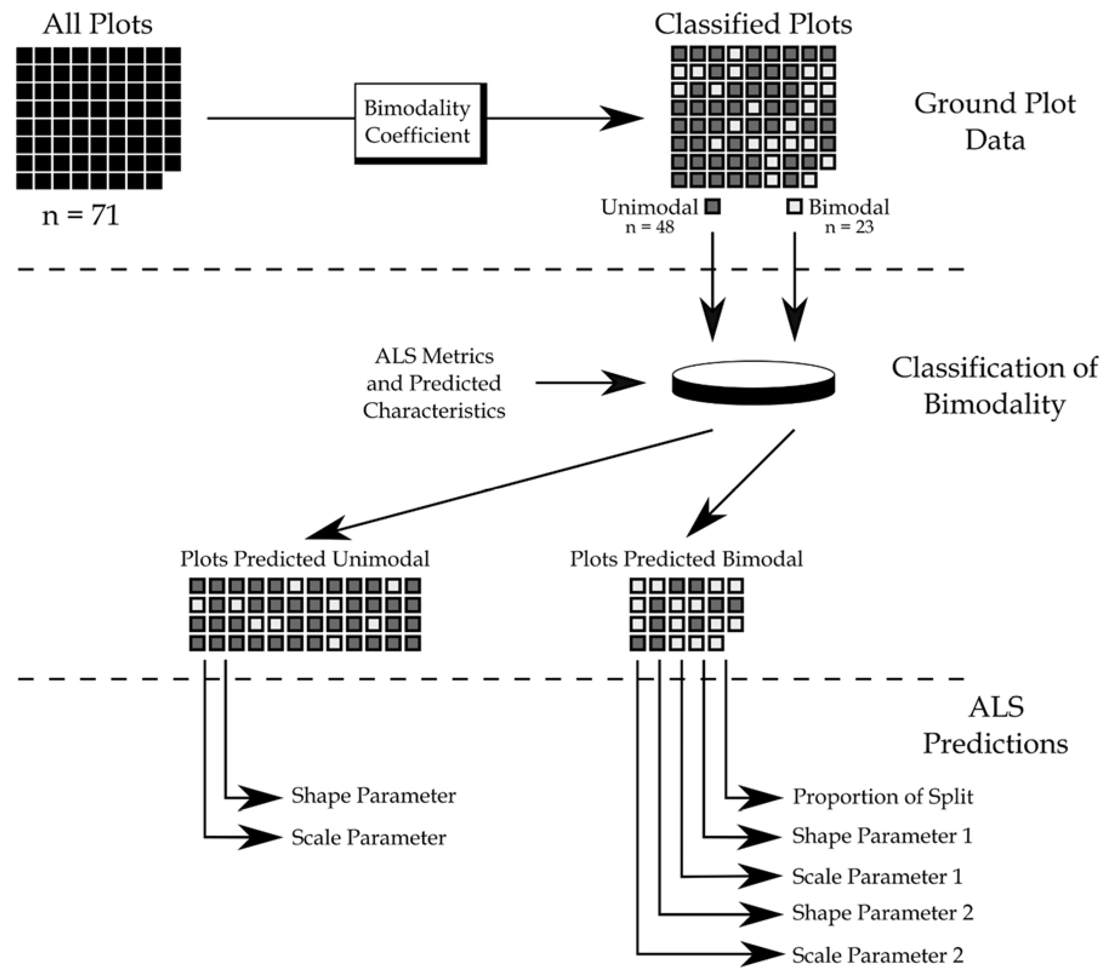
2.4. Analysis Approach

Figure 2 summarizes the workflow applied. The measured trees within each ground plot were first combined into 2-cm diameter classes and classified as either unimodal or bimodal using the bimodality coefficient. Then, various stand characteristics, measured on plots and predicted using ALS, were assessed for their ability to identify the plots as either unimodal or bimodal. Once the best ALS metric for identification was determined, it was used to categorize plots for estimation of SSD parameters by ALS. Field-based SSDs on classified plots were used as response data for prediction with ALS metrics. Each of these steps is described in further detail below.

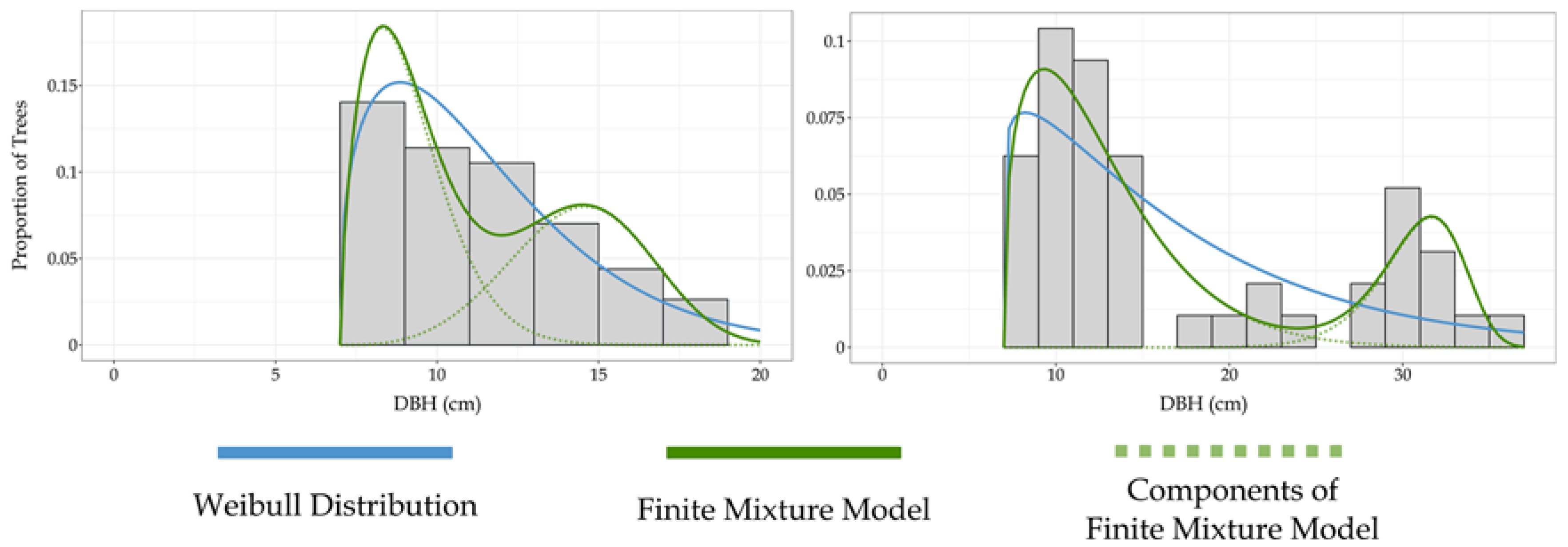
2.5. Differentiation of Modality in Stem Size Distributions

Stands classified as multimodal are thought to be highly variable and structurally heterogeneous, and this heterogeneity has been quantified in different ways (

Table 4. Published predictors of multimodal diameter distributions and how they are used to classify bimodal plots. DBH, diameter at breast height.

Differentiation	Source	Quantified as
Uneven-aged stands	Zhang et al. 2001 [13]	Std. dev. of ages (SDA)
Mixed-species stands	Liu et al. 2002 [14]	% Dominant species
Density/Height Ratio	Thomas et al. 2008 [15]	N/top height (D/H)
Multilayered	Podlaski 2010 [11]	Std. dev. of heights (SDH)
Varied diameters	Maltamo and Gobakken 2014 [12]	Std. dev. of DBHs (SDDBH)

). We examined how effective each of the characteristics identified in Table 4 were for differentiating between unimodal and bimodal SSD using both ground measurements and ALS-derived predictions of the five characteristics for differentiation. In an operational context, the use of a single ALS metric would be advantageous if it could be used as an effective heuristic to identify unimodal and bimodal grid cells, because a single metric would be available wall-to-wall (wherever ALS data is acquired), would be generated as a standard preliminary processing step for an area-based approach (described below), and would require no ground samples or additional modelling.

First, as a baseline, five ground-measured characteristics were assessed for their ability to discriminate unimodal and bimodal plots. Next, using an area-based approach, predictive models were developed to estimate each of the five ground-measured characteristics in Table 4 using ALS metrics (Table 3) as predictors and the ground-measured characteristics as response variables. Models were built using stepwise linear regression, and final models were selected based on combinations of up to three metrics (to avoid overfitting) that captured the most variation in the sample population. Predictor variables were selected so that those showing a strong correlation (r > 0.8; [45]) with each other or coming from the same category of descriptors were not included in the same model. The accuracy of area-based models for each of the aforementioned characteristics was assessed in terms of an adjusted r² and relative Root Mean Square Error (RMSE) for all sample plots. Finally, individual ALS metrics were used to differentiate SSD modality.

2.6. Accuracy of Modality Differentiation

Modality differentiation was assessed by determining the overall accuracy of the classification that each measure produced. The classification accuracy was defined as the percentage of all PSPs that were correctly classified as either unimodal or bimodal. This was assessed for each characteristic and ALS metric, and allowed for consistent comparison between structural characteristics and individual metrics. A successful classification was defined as a statistically significant improvement from no classification (i.e. if we assume all plots are unimodal). The exact binomial test was used to assess the statistical difference between each classification method and the classification of all plots as unimodal [46].

2.7. Predictive Modeling of SSD Parameters Using ALS Metrics

Once a SSD of a plot was classified as either unimodal or bimodal using the most accurate ALS model, a structurally appropriate distribution function was fit to the ground-measured SSD (Figure 3). As complete data in the study area exists for trees > 7 cm DBH, a truncated Weibull distribution was used for describing the SSD in unimodal stands, with the truncation point set at 7 cm [47]. While nonparametric imputations such as k-NN and Random Forest have been used to predict SSDs [48], these typically require large amounts of samples to be taken [49]. Instead, a Finite Mixture Model (FMM), which applies k separate distributions to k components of data that are split at statistical breakpoints, where k is the number of modes in the data [14], was used for the bimodal distributions (i.e., k = 2). Similar to Thomas et al. [15], separate Weibull distributions were fit using MLE. Once the parameters of the appropriate distributions were estimated from the measured DBHs, the parameters were used to develop area-based models from the ALS metrics in order to estimate the PDF parameters and the SSD across the management area.

2.8. Evaluation of SSD Parameters Using the Error Index (EI)

To examine the fit of the ALS-predicted SSD to the original measured tree stem DBHs, the Error Index (EI) proposed by Reynolds et al. [50] was used. The EI reports the sum of observed differences in each class as a proportion of the number of trees at a site. The EI is a frequently used method of evaluating SSD functions, as it allows for comparison across different fitting techniques (e.g., [51]) or PDFs (e.g., [32]). Two different EI calculations were used—one to compare fits of ground-measured distributions (EI_G, Equation 2) and one to compare fits of ALS-estimated distributions (EI_ALS, Equation 3):

$${\mathit{EI}}_G={\displaystyle \sum }_{i=1}^{m}100\left|\frac{f_{\mathit{REF}i}-f_{\mathit{PDF}i}}{n_{\mathit{REF}i}}\right|,$$

(2)

$$E{I}_{ALS}= {\displaystyle \sum }_{i=1}^{m}100\left|\frac{f_{REF i}}{n_{REF i}}-\frac{f_{ALS i}}{n_{ALS i}}\right|,$$

(3)

where f_REFi is the measured frequency in DBH class i, f_PDFi is the PDF-derived frequency in DBH class i, f_ALSi is the estimated frequency in DBH class i, n_REFi is the total number of measured stems in class i, and n_ALS is the total number of estimated stems in class i. EI_ALS was determined following Packalén and Maltamo [19], with n_ALS determined using an area-based approach and the same variables used for the PDF parameter estimation. Both error indices range from 0, indicating a perfect fit, to 200, indicating non-overlapping distributions.

3. Results

3.1. Differentiation of Modality in Stem Size Distributions

Most of the metrics and models were successful in differentiating plots into either unimodal or bimodal distributions (

Table 5. Accuracy of bimodal plots classification using ground measurements, ALS predictions, and corresponding ALS metrics.

	Differentiation	Overall Accuracy	ALS Prediction Accuracy
			Adj. r2	% RMSE
Plot Data	SDA	59.2	-	-
	% Dominant Species	59.2	-	-
	D/H	64.8	-	-
	SDH	67.6	-	-
	SDDBH	70.4	-	-
ALS Predictions	SDA	66.2	0.059	88.4
	% Dominant Species	63.4	0.155	27.3
	D/H	74.7 *	0.600	43.8
	SDH	67.6	0.694	25.7
	SDDBH	74.7 *	0.640	31.2
ALS Metrics	Variance	77.5 *	-	-
	Kurtosis	46.5	-	-
	Canopy Relief Ratio	57.8	-	-
	% All Returns >2 m.	63.4	-	-
	Filling Ratio	66.2	-	-
	Rumple	74.7 *	-	-

* indicates a significant improvement from no classification (i.e. assuming all plots are unimodal). SD_A is the standard deviation of ages, D/H is the density divided by top height, SD_H is the standard deviation of ages, and SD_DBH is the standard deviation of DBH’s.

). SD_DBH and the SD_H had the highest overall classification accuracy (70.4% and 67.6%, respectively) of the ground-measured metrics, while the SD_A and % dominant species had the lowest accuracy (both 59.2%).

Characteristics related to tree size variability (SD_H, SD_DBH, D/H) were most accurately predicted by ALS (Adj. r² > 0.6), while as expected, characteristics not related to tree dimensions (SD A , % dominant species) had poorest predictions (Adj. r² < 0.2). In terms of their capacity to discriminate modality, the best ALS-predicted characteristic was SD_DBH (74.7%), while the poorest was % dominant species (63.4%). Of the individual ALS metrics used to differentiate modality, the variance of ALS return heights was the most accurate (77.5%) and provided the most accurate differentiation overall. The variance of ALS return heights was therefore selected for differentiating modality for the remainder of the study.

3.2. Predictive Modeling of SSD Parameters Using ALS Metrics

The adjusted r² values for the predicted Weibull and FMM parameters were similar (0.5–0.6) with the exception of the unimodal shape parameter and the shape parameter for the second group of the FMM (0.3925 and 0.2019, respectively;

Table 6. Prediction accuracy of SSD parameters for unimodal (n = 48) and bimodal (n = 23) plots as differentiated by ALS.

Parameter		Prediction Accuracy
		Adj. r2	% RMSE
Unimodal	Shape	0.3925	23.26
	Scale	0.6271	30.39
Bimodal	Shape1	0.5497	30.25
	Scale1	0.5898	32.86
	Shape2	0.2019	33.93
	Scale2	0.5203	29.81
	% over breakpoint	0.5389	42.91

). Although each of the metrics in Table 3 was used in at least one predictive model, some appeared more frequently than others. The most frequently used metrics were P95, Kurtosis, % All Returns Above 2 m, and the Filling Ratio.

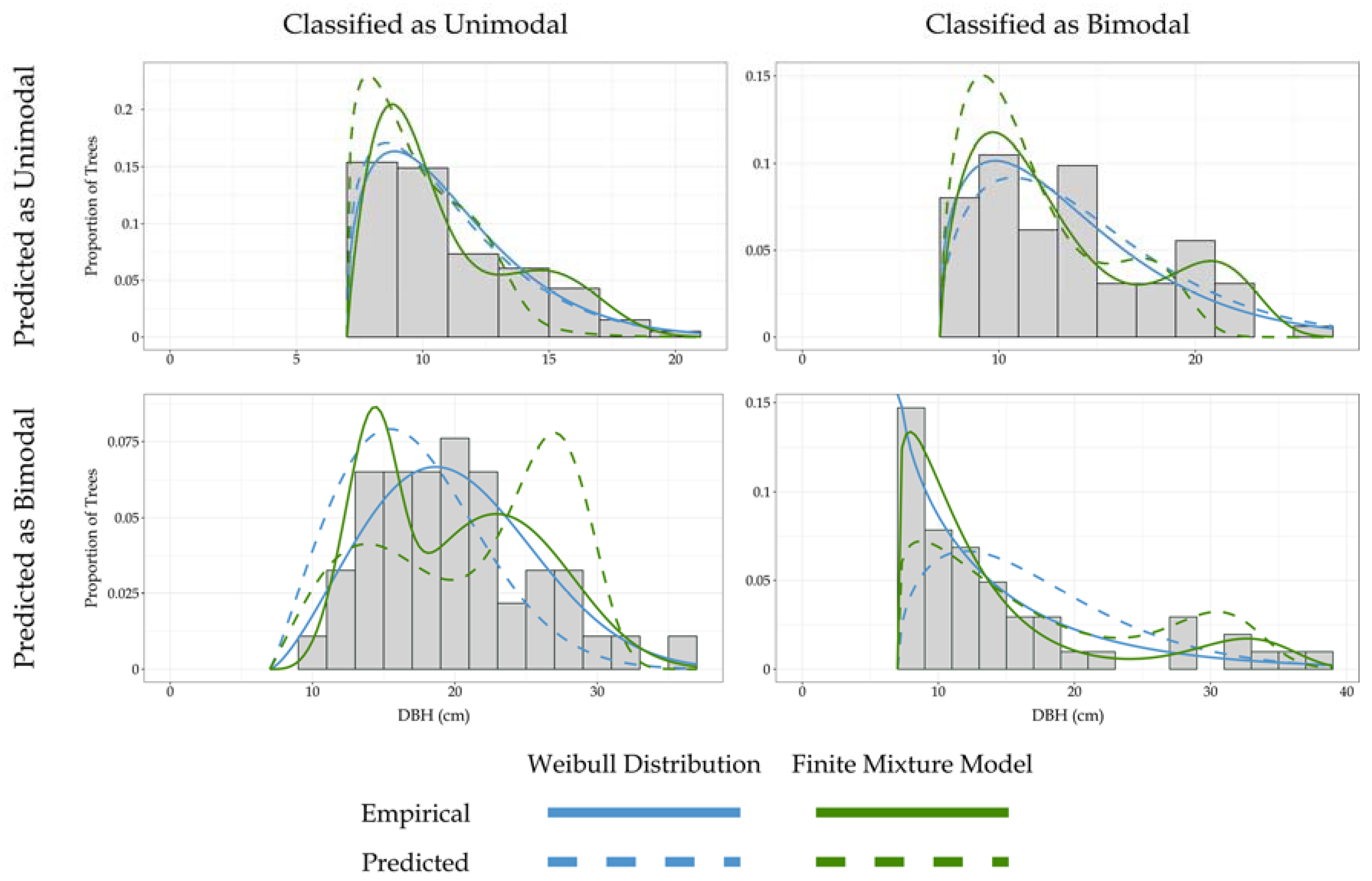
3.3. Accuracy of Predicted Distributions

Using a mixture model on bimodal plots resulted in a higher accuracy than using a unimodal distribution on all plots for both ground-measured and ALS-predicted parameters (

Table 7. Measured (EI_G) and predicted (EI_ALS) values on sample plots, showing differences in unimodal and bimodal plots.

	Ground Fstimates (EIG)	ALS Predictions (EIALS)
Mean EI (unimodal plots)	25.29	42.86
Mean EI (bimodal plots)	34.30	62.21
Mean EI (all plots)	28.20	49.13
Mean EI (unimodal Weibull on all plots)	31.24	51.31

; Figure 4). For ground-measured plots, the mean EI_G was 28.20 using mixture models and unimodal distributions when appropriate, while only using a unimodal distribution would have resulted in an EI_G value of 31.24. Similarly, the mean EI_ALS was 49.13 after differentiating modality, while predicting only a unimodal distribution on all plots would have resulted in a mean EI_ALS value of 51.31. Plots deemed bimodal based on ground measurements and ALS predictions had higher mean error values than unimodal plots, with a difference of 9.01 between EI_G values and 19.35 between EI_ALS values.

4. Discussion

4.1. Differentiation of Modality in Stem Size Distributions

The fact that neighboring stands in the boreal mixedwood forest can have vastly different structures requires flexible and spatially detailed approaches to SSD estimation. Field campaigns to measure SSD across large, diverse, and often remote areas are not feasible given constraints on time and resources. In addition, a priori knowledge of an appropriate PDF to use for fitting the SSD would be valuable when operating in structurally diverse areas. The methodology outlined in this study provides the ability to quickly and effectively characterize diverse forests over large spatial extents by providing detailed measures of the vertical distribution of vegetation over large areas using ALS data.

The ground-measured variables best able to differentiate bimodal distributions were those relating to tree sizes, such as SD_H and SD_DBH. This is consistent with estimating SSD, which represents the variation in tree DBH. If a stand has highly variable tree sizes, there will be a correspondingly large variance in DBHs and heights, likely reflecting in a multimodal SSD. Age variability and species mixtures provided less accurate differentiations, as maturing stand structure depends more on disturbance trends and ecological legacies than species or age differences [16,17].

Likewise, the most accurate ALS predictions of plot characteristics came from those related to tree size. This was expected, as ALS metrics best characterize physical structure and have more difficulty in estimating intrinsic characteristics such as the age or species of a tree. While attributes such as the percent dominant species and the SD of ages can be used to classify bimodal plots at the ground level, they are not predicted very accurately with ALS, which limits their use at an operational capacity. The variance of ALS heights performed the best in classifying bimodal plots and was chosen as the preferred determinant of modality in this study. This metric is commonly calculated as part of the standard suite of ALS metrics generated from software packages such as LAStools [52] and FUSION [36]. Consequently, it is easily generated, accessible, and readily interpretable as a heuristic for distinguishing modality. While alternative approaches to modality characterization could include logistic regression or other modeling techniques, the parsimony, consistency, and transferability of a single metric makes our approach more applicable in other study areas and research. Further work could investigate more detailed ALS-based stratification of the study area to appropriately model other forest characteristics in addition to SSD.

4.2. Predictive Modeling of SSD Parameters Using ALS Metrics

The parameters of the Weibull and FMM distributions were predicted well using ALS-derived metrics. Thomas et al. [15] predicted Weibull and FMM parameters using ALS in a similar study area and achieved similar or slightly more accurate results for parameter predictions. However, their study first stratified by species and structural groups and predictive models included up to seven variables, whereas we used no more than three input variables in our models and did not stratify by species groups. Applying predictions across the landscape using the approach of Thomas et al. [15] would require the availability of reliable species information at the same spatial resolution as the ALS data, which can be difficult or expensive to acquire. Likewise, the current capacity of ALS does not allow for accurate and spatially detailed species characterization, making stratification by species often not feasible.

There was a large difference in prediction accuracy among parameters of the same model. Given the pulse density of our ALS data and the number of sample plots that were available, it was difficult to accurately predict all five FMM parameters, and these distributions had a wide range of resulting curves. In a few cases, the resulting distribution was one that imprecisely characterized the ground-measured SSD. However, ALS data with higher point densities should be able to capture more variation within sample plots and more accurately characterize bimodal plots.

4.3. Accuracy of Predicted SSDs

The aforementioned discrepancies in prediction accuracy of SSD parameters likely compounded the errors of distributions fitted to ALS data. Thus, the mean EI_ALS value for bimodal plots was slightly higher than that for unimodal plots. However, the methodology used in this study produced more accurate results in terms of both EI_G and EI_ALS than if all plots had been classified as unimodal. The difference in EI_ALS values was relatively low for predicted distributions and slightly higher for measured distributions; this suggests that the accuracy of a predicted SSD decreases with decreasing parameter prediction accuracy. Thomas et al. [15] did not report EI values; however, a study by Tompalski et al. [42] reported similar EI_ALS values to those reported herein when predicting SSD for unimodal distributions. Tompalski et al. [42] scaled EI values by 0.5 while we used 100 (Equation 3). When correcting for this difference in scale, our mean EI_ALS values were slightly more accurate than those reported by Tompalski et al. [42], whose mean value was 71.6.

4.4. Model Application

Unless a stand is small or completely homogeneous, a single plot-level SSD will likely not be representative of SSD for the stand [53]. Therefore, techniques for the aggregation of predictions from cell-level SSD are necessary to generate a stand-level SSD. One such approach involves summing predicted SSDs from each grid cell composing a delineated stand [54]. More complex approaches involve multidimensional scaling [55], in which an estimator can be used for extrapolation to larger units, or segmenting areas into smaller units such as microstands, which are areas grouped by similar ALS-predicted attributes such as volume and height [56]. If stand-level predictions are the desired result, a final aggregation step should be used to scale up from cell-level predictions; however, this was beyond the scope of the current study and SSD predictions remained at the cell level.

5. Conclusions

The structurally complex SSDs that exist in the boreal mixedwood forest should be fit with correspondingly complex distribution models. The difference in structures among stands requires detailed, landscape-level information to guide the fitting and modeling process. In order to meet the scope and detail needed for accurate forest management decisions, we used ALS as a means of differentiating and predicting SSD parameters in a boreal mixedwood forest. The differentiation step allowed us to fit structurally appropriate SSDs to respective stands and allowed for more robust characterizations of SSD than using a single model for the entire study area. For forest professionals who rely on detailed stand-level information, differentiating bimodal areas and their subsequent characterization by FMMs should provide insights into stand characteristics that would lead to more informed decisions and more accurate understanding of stand structure in complex habitats.

References

1. Hyyppä, J.; Hyyppä, H.; Leckie, D.; Gougeon, F.; Yu, X.; Maltamo, M. Review of methods of small-footprint airborne laser scanning for extracting forest inventory data in boreal forests. Int. J. Rem. Sens. 2008, 29, 1339–1366. [Google Scholar] [CrossRef]
2. Taubert, F.; Hartig, F.; Dobner, H.-J.; Huth, A. On the challenge of fitting tree size distributions in ecology. PLoS ONE 2013, 8, e58036. [Google Scholar] [CrossRef] [PubMed]
3. Gobakken, T.; Næsset, E. Estimation of diameter and basal area distributions in coniferous forest by means of airborne laser scanner data. Scand. J. For. Res. 2004, 19, 529–542. [Google Scholar] [CrossRef]
4. Hetemäki, L.; Mery, G.; Holopainen, M.; Hyyppä, J.; Vaario, L.-M.; Yrjälä, K. Implications of Technological Development to Forestry; IUFRO (International Union of Forestry Research Organizations) Secretariat: Vienna, Austria, 2010; Volume 25, ISBN 3-901347-93-3. [Google Scholar]
5. Nduwayezu, J.; Mafoko, G.; Mojeremane, W.; Mhaladi, L. Vanishing multipurpose indigenous trees in Chobe and Kasane forest reserves of Botswana. Resour. Environ. 2015, 5, 167–172. [Google Scholar]
6. Landsberg, J.; Mäkelä, A.; Sievänen, R.; Kukkola, M. Analysis of biomass accumulation and stem size distributions over long periods in managed stands of Pinus sylvestris in Finland using the 3-PG model. Tree Physiol. 2005, 25, 781–792. [Google Scholar] [CrossRef] [PubMed]
7. Garcıa, O. What is a diameter distribution? In Proceedings of the Symposium on Integrated Forest Management Information Systems; International Union of Forest Research Organizations: Tsukuba, Japan, 1992; pp. 11–29. [Google Scholar]
8. Brandt, J.; Flannigan, M.; Maynard, D.; Thompson, I.; Volney, W. An introduction to Canada’s boreal zone: ecosystem processes, health, sustainability, and environmental issues. Environ. Rev. 2013, 21, 207–226. [Google Scholar] [CrossRef]
9. Coomes, D.A.; Duncan, R.P.; Allen, R.B.; Truscott, J. Disturbances prevent stem size-density distributions in natural forests from following scaling relationships. Ecol. Lett. 2003, 6, 980–989. [Google Scholar] [CrossRef]
10. Freeman, J.B.; Dale, R. Assessing bimodality to detect the presence of a dual cognitive process. Behav. Res. Methods 2013, 45, 83–97. [Google Scholar] [CrossRef] [PubMed]
11. Podlaski, R. Suitability of the selected statistical distributions for fitting diameter data in distinguished development stages and phases of near-natural mixed forests in the Świętokrzyski National Park (Poland). For. Ecol. Manag. 2006, 236, 393–402. [Google Scholar] [CrossRef]
12. Maltamo, M.; Gobakken, T. Predicting tree diameter distributions. In Forestry Applications of Airborne Laser Scanning; Springer: Dordrecht, The Netherlands, 2014; pp. 177–191. [Google Scholar]
13. Zhang, L.; Gove, J.H.; Liu, C.; Leak, W.B. A finite mixture of two Weibull distributions for modeling the diameter distributions of rotated-sigmoid, uneven-aged stands. Can. J. For. Res. 2001, 31, 1654–1659. [Google Scholar] [CrossRef]
14. Liu, C.; Zhang, L.; Davis, C.J.; Solomon, D.S.; Gove, J.H. A finite mixture model for characterizing the diameter distributions of mixed-species forest stands. For. Sci. 2002, 48, 653–661. [Google Scholar]
15. Thomas, V.; Oliver, R.; Lim, K.; Woods, M. LiDAR and Weibull modeling of diameter and basal area. For. Chron. 2008, 84, 866–875. [Google Scholar] [CrossRef]
16. Kane, V.R.; Bakker, J.D.; McGaughey, R.J.; Lutz, J.A.; Gersonde, R.F.; Franklin, J.F. Examining conifer canopy structural complexity across forest ages and elevations with LiDAR data. Can. J. For. Res. 2010, 40, 774–787. [Google Scholar] [CrossRef]
17. Franklin, J.F.; Spies, T.A.; Van Pelt, R.; Carey, A.B.; Thornburgh, D.A.; Berg, D.R.; Lindenmayer, D.B.; Harmon, M.E.; Keeton, W.S.; Shaw, D.C. Disturbances and structural development of natural forest ecosystems with silvicultural implications, using Douglas-fir forests as an example. For. Ecol. Manag. 2002, 155, 399–423. [Google Scholar] [CrossRef]
18. Bailey, R.L.; Dell, T. Quantifying diameter distributions with the Weibull function. For. Sci. 1973, 19, 97–104. [Google Scholar]
19. Myung, I.J. Tutorial on maximum likelihood estimation. J. Math. Psychol. 2003, 47, 90–100. [Google Scholar] [CrossRef]
20. Packalén, P.; Maltamo, M. Estimation of species-specific diameter distributions using airborne laser scanning and aerial photographs. Can. J. For. Res. 2008, 38, 1750–1760. [Google Scholar] [CrossRef]
21. Penner, M.; Woods, M.; Pitt, D.G. A comparison of airborne laser scanning and image point cloud derived tree size class distribution models in boreal Ontario. Forests 2015, 6, 4034–4054. [Google Scholar] [CrossRef]
22. Eid, T.; Gobakken, T.; Næsset, E. Comparing stand inventories for large areas based on photo-interpretation and laser scanning by means of cost-plus-loss analyses. Scand. J. For. Res. 2004, 19, 512–523. [Google Scholar] [CrossRef]
23. White, J.C.; Coops, N.C.; Wulder, M.A.; Vastaranta, M.; Hilker, T.; Tompalski, P. Remote sensing technologies for enhancing forest inventories: A review. Can. J. Rem. Sens. 2016, 42, 619–641. [Google Scholar] [CrossRef]
24. Næsset, E. Predicting forest stand characteristics with airborne scanning laser using a practical two-stage procedure and field data. Rem. Sens. Environ. 2002, 80, 88–99. [Google Scholar] [CrossRef]
25. Næsset, E. Airborne laser scanning as a method in operational forest inventory: Status of accuracy assessments accomplished in Scandinavia. Scand. J. For. Res. 2007, 22, 433–442. [Google Scholar] [CrossRef]
26. Van Leeuwen, M.; Nieuwenhuis, M. Retrieval of forest structural parameters using LiDAR remote sensing. Eur. J. For Res. 2010, 129, 749–770. [Google Scholar] [CrossRef]
27. Maltamo, M.; Packalén, P.; Yu, X.; Eerikäinen, K.; Hyyppä, J.; Pitkänen, J. Identifying and quantifying structural characteristics of heterogeneous boreal forests using laser scanner data. For. Ecol. Manag. 2005, 216, 41–50. [Google Scholar] [CrossRef]
28. Kao, D.L.; Kramer, M.G.; Love, A.L.; Dungan, J.L.; Pang, A.T. Visualizing distributions from multi-return lidar data to understand forest structure. Cartogr. J. 2005, 42, 35–47. [Google Scholar] [CrossRef]
29. Maltamo, M.; Suvanto, A.; Packalén, P. Comparison of basal area and stem frequency diameter distribution modelling using airborne laser scanner data and calibration estimation. For. Ecol. Manag. 2007, 247, 26–34. [Google Scholar] [CrossRef]
30. Natural Regions Committee Natural Regions and Subregions of Alberta. Compiled by DJ Downing and WW Pettapiece; Government of Alberta: Edmonton, Canada, 2006.
31. Forest Management Branch. Permanent Sample Plot (PSP) Field Procedures Manual; Alberta Sustainable Resource Development, Public Lands and Forest Division: Edmonton, Canada, 2005.
32. Zhang, L.; Packard, K.C.; Liu, C. A comparison of estimation methods for fitting Weibull and Johnson’s SB distributions to mixed spruce fir stands in northeastern North America. Can. J. For. Res. 2003, 33, 1340–1347. [Google Scholar] [CrossRef]
33. SAS Institute. SAS/STAT User’s Guide; SAS Institute Inc.: Cary, NC, USA, 1989. [Google Scholar]
34. Ellison, A.M. Effect of seed dimorphism on the density-dependent dynamics of experimental populations of Atriplex triangularis (Chenopodiaceae). Am. J. Bot. 1987, 1280–1288. [Google Scholar] [CrossRef]
35. Axelsson, P. DEM generation from laser scanner data using adaptive TIN models. Int. Arch. Photogramm. Rem. Sens. 2000, XXXIII, 110–117. [Google Scholar]
36. McGaughey, R.J. FUSION/LDV: Software for LIDAR Data Analysis and Visualization; US Department of Agriculture, Forest Service, Pacific Northwest Research Station: Seattle, WA, USA, 2009; p. 123.
37. R Core Team. R: A language and environment for statistical computing; R Foundation for Statistical Computing: Vienna, Austria, 2016. [Google Scholar]
38. Roussel, J.R.; Auty, D. lidR: Airborne LiDAR Data Manipulation and Visualization for Forestry Applications. R package. Available online: https://github.com/Jean-Romain/lidR (accessed on 31 January 2018).
39. Kane, V.R.; McGaughey, R.J.; Bakker, J.D.; Gersonde, R.F.; Lutz, J.A.; Franklin, J.F. Comparisons between field-and LiDAR-based measures of stand structural complexity. Can. J. For. Res. 2010, 40, 761–773. [Google Scholar] [CrossRef]
40. Tompalski, P. Wykorzystanie wskaźników przestrzennych 3D w analizach cech roślinności miejskiej na podstawie danych z lotniczego skanowania laserowego. Archiwum Fotogrametrii, Kartografii i Teledetekcji 2012, 23. [Google Scholar]
41. Van Ewijk, K.Y.; Treitz, P.M.; Scott, N.A. Characterizing forest succession in Central Ontario using LiDAR-derived indices. Photogramm. Engin. Rem. Sens. 2011, 77, 261–269. [Google Scholar] [CrossRef]
42. Tompalski, P.; Coops, N.C.; White, J.C.; Wulder, M.A. Enriching ALS-derived area-based estimates of volume through tree-level downscaling. Forests 2015, 6, 2608–2630. [Google Scholar] [CrossRef]
43. Bouvier, M.; Durrieu, S.; Fournier, R.A.; Renaud, J.-P. Generalizing predictive models of forest inventory attributes using an area-based approach with airborne LiDAR data. Rem. Sens. Environ. 2015, 156, 322–334. [Google Scholar] [CrossRef]
44. Popescu, S.C.; Zhao, K. A voxel-based lidar method for estimating crown base height for deciduous and pine trees. Rem. Sens. Environ. 2008, 112, 767–781. [Google Scholar] [CrossRef]
45. Van Aardt, J.A.; Wynne, R.H.; Oderwald, R.G. Forest volume and biomass estimation using small-footprint lidar-distributional parameters on a per-segment basis. For. Sci. 2006, 52, 636–649. [Google Scholar]
46. Aronoff, S. Classification accuracy: A user approach. Photogramm. Eng. Rem. Sens. 1982, 48, 1299–1307. [Google Scholar]
47. McGarrigle, E.; Kershaw, J.A., Jr.; Lavigne, M.B.; Weiskittel, A.R.; Ducey, M. Predicting the number of trees in small diameter classes using predictions from a two-parameter Weibull distribution. Forestry 2011, 84, 431–439. [Google Scholar] [CrossRef]
48. Bollandsås, O.M.; Maltamo, M.; Gobakken, T.; Næsset, E. Comparing parametric and non-parametric modelling of diameter distributions on independent data using airborne laser scanning in a boreal conifer forest. Forestry 2013, 86, 493–501. [Google Scholar] [CrossRef]
49. Maltamo, M.; Næsset, E.; Bollandsås, O.M.; Gobakken, T.; Packalén, P. Non-parametric prediction of diameter distributions using airborne laser scanner data. Scand. J. For. Res. 2009, 24, 541–553. [Google Scholar] [CrossRef]
50. Reynolds, M.R.; Burk, T.E.; Huang, W.-C. Goodness-of-fit tests and model selection procedures for diameter distribution models. For. Sci. 1988, 34, 373–399. [Google Scholar]
51. Palahí, M.; Pukkala, T.; Trasobares, A. Modelling the diameter distribution of Pinus sylvestris, Pinus nigra and Pinus halepensis forest stands in Catalonia using the truncated Weibull function. Forestry 2006, 79, 553–562. [Google Scholar] [CrossRef]
52. Isenburg, M. Lastools-efficient LiDAR processing software. Available online: lastools.org (accessed on 10 October 2017).
53. Borders, B.E.; Wang, M.; Zhao, D. Problems of scaling plantation plot diameter distributions to stand level. For. Sci. 2008, 54, 349–355. [Google Scholar]
54. Siipilehto, J.; Lindeman, H.; Vastaranta, M.; Yu, X.; Uusitalo, J. Reliability of the predicted stand structure for clear-cut stands using optional methods: Airborne laser scanning-based methods, smartphone-based forest inventory application Trestima and pre-harvest measurement tool EMO. Silva Fennica 2016, 50. [Google Scholar] [CrossRef]
55. Magnussen, S.; Renaud, J.-P. Multidimensional scaling of first-return airborne laser echoes for prediction and model-assisted estimation of a distribution of tree stem diameters. Ann. For. Sci. 2016, 73, 1089–1098. [Google Scholar] [CrossRef]
56. Lundholm, A. Evaluating Inventory Methods for Estimating Stem Diameter Distributions in Micro Stands Derived from Airborne Laser Scanning. Master’s Thesis, Sveriges lantbruksuniversitet, Umeå, Sweden, 2014. [Google Scholar]
Figure 1. Map of the Slave Lake study area and sample plots (n = 71).
Forests 09 00095 g001
Figure 2. Workflow for differentiating bimodal plots and estimating stem size distribution (SSD) parameters with ALS.
Forests 09 00095 g002
Figure 3. Weibull distributions (blue) best fit unimodal stands (left), while more complex distributions such as a Finite Mixture Model (green) best fit multimodal stands (right).
Forests 09 00095 g003
Figure 4. Examples of measured and predicted curves following correct and incorrect differentiation on four plots.
Forests 09 00095 g004