Spatial Segregation Facilitates the Coexistence of Tree Species in Temperate Forests

Abstract

Competition between plants has an important role during the natural succession of forest communities. Niche separation between plants can reduce such interspecific competition and enable multispecies plant to achieve coexistence, although this proposition has rarely been supported in experiments. Plant competition can be captured by spatial segregation of the competing species to avoid fierce direct conflicts for nutrients and light. We investigated a site of 400 m × 1000 m in Beijing Pine Mountain National Nature Reserve that was established for protecting Chinese pine and some rare fungi. Six dominant tree species (Fraxinus chinensis Roxb., Syringa reticulata (Blume) H. Hara var. amurensis (Rupr.) J. S. Pringle, Quercus mongolica Fisch. ex Ledeb., Armeniaca sibirica (L.) Lam., Pinus tabuliformis Carrière, and Ulmus pumila L.) were individually marked. Metrics of spatial segregation, based on the theory of spatial point process, were calculated to detect spatial competition. The corresponding type (species)-specific probabilities and the p-values from a spatially implicit test revealed significant overall spatial segregation between the six tree species. We further used the cross-type L-function to check the spatial correlation between Chinese pine and the other tree species, and detected a significant spatial repulsion relationship with four other tree species. Our study shows that each of the six dominant tree species occupies a different subarea in the landscape to effectively reduce direct spatial competition. We thus argue that patchy distributions of different tree species could be common in late forest community succession, and the coexistence of plants could be maintained over a large spatial scale. Management intervention, such as thinning the densities of dominant tree species, could be used to foster species coexistence and ensure the productivity of commercial stands.

1. Introduction

Patchy distributions of individuals in forest communities are typical, driven largely by competition and disturbance [1,2]. Understanding how competition and disturbance jointly affect species persistence and distribution can help to address many management challenges, such as the protection of rare species [3], the control of biological invasions [4], and the prediction of the effects of climate change [5]. The two-species Lotka–Volterra model predicts only two results from competition: stable coexistence or the stronger competitor repels the weaker one [6]. Similarly, multispecies Lotka–Volterra competition model predicts either coexistence or extinctions of some species [7]. However, such Lotka–Volterra models are spatially inexplicit and thus neglect, in most cases, the effects of spatial scale, heterogeneity, and disturbance on the consequence of competition. In natural forests, however, the weaker competitors can be compensated by being stronger dispersers or colonizers from r-selection [8]. Moreover, human and/or natural disturbance could create temporally available empty habitats for these stronger dispersers but weaker competitors to recruit. Consequently, other mechanisms are available to foster coexistence by inducing niche differentiation and negative frequency dependence [9], such as the response to the variation of spatiotemporal environments [10], the division of resources, and the endemic natural alkenes of species in natural forests [11]. With distance-limited dispersal and spatially autocorrelated habitat heterogeneity, these coexistence mechanisms could then lead to the signature pattern of spatial segregation in forest communities.

Spatial point pattern analysis is an important technique to explore the interspecific and intraspecific relationship in space [12,13,14]. If the count data of plants on a given scale are random in different subregions, the Poisson distribution can be deployed for description; this is usually regarded as the null hypothesis [15]. If there exists some levels of spatial clustering or repulsion, the null hypothesis will be violated. In this case, Ripley’s K function becomes the most widely used method in forest ecology [16], which can distinguish three types of spatial distributions: clustering, randomness, and regular distributions of individuals [17]. It has been extended further to analyze interspecific spatial relationship by considering multivariate point processes [13]. Recent developments have extended the use of K-function for analyzing the spatiotemporal point patterns [12], even though such an extension appears to be more appropriate for examining the spatial dynamics and intra- or interspecific spatial relationships of seedlings or plants with short recruitment periods (e.g., herbaceous plants).

For the typical data of forest inventories, the temporal turnover of trees is usually caused by environmental disturbance, and thus does not reflect the results from competition as the duration of forestry survey is often much shorter than the life span of trees. For forest communities without frequent disturbances, community structures could experience substantial changes on small scales. On large scales, such changes of tree compositions can be minuscule from year on year. A 10-year interval, however, could be enough to study the spatiotemporal changes of trees. However, in practice, for most forest inventory data with one snapshot survey, spatial analysis is the more useful for forest ecology and management (e.g., ref. [18]). To test for spatial segregation, a nonparametric kernel estimation method was proposed, which has been used to test for spatial segregation among the spoligotypes of bovine tuberculosis and moso bamboos with different ages, among others [19,20,21,22]. However, this method has not been paid enough attention in forest research.

Chinese pine (Pinus tabuliformis Carrière) is a native conifer in northern China. It has been used as an indicator species for the investigation of climate change effects on forest ecosystems [1,23,24]. Only few studies have explored the spatial competition between the Chinese pine and other co-occurring species. Given the important ecological and economic values of Chinese pines in regional forest communities, it is necessary to explore its spatial relationship with other co-occurring tree species on a reasonable spatial scale. In this paper, we explored the spatial relationships among dominant tree species using a large natural forest site of 400 m × 1000 m where Chinese pine was a dominant species.

2. Materials and Methods

2.1. Study Site

The study site is located within the Beijing Pine Mountain National Nature Reserve (40°30′50″ N, 115°49′12″ E); the reserve was established in 1985, and is located in Yanqing County, Beijing, China. In August 2014, we delineated all trees with the diameter at breast height (DBH) ≥2 cm within a landscape of 400 m × 1000 m (made up of one-thousand 20 m × 20 m plots). DBHs and locations of trees were recorded. In the following, we count the abundances of tree species, calculate the level of spatial segregation between given pairs of dominant tree species, and compute the spatial correlations of these dominant tree species. We also considered two subregions, [0, 400] × [0, 400] and [0, 400] × [600, 1000], taken from the study area [0, 400] × [0, 1000], for our analyses.

2.2. Statistical Methods

2.2.1. Species-Specific Probabilities for Spatial Segregation

Diggle et al. proposed a method to test spatial segregation using multivariate point processes [19]. Spatial segregation is defined in a multivariate point pattern if, for at least some species, j ≠ i, where the conditional intensity of species j at location x given species i at x is less than the marginal intensity of species j at x. A type-specific probability was defined as the conditional probability that a case known to occur at x is of type k:

$$p_k(x)=\frac{{\mathsf{\lambda }}_k(x)}{{\displaystyle \sum _{j=1}^m{\mathsf{\lambda }}_j(x)}}=\frac{{\rho }_k(x)}{{\displaystyle \sum _{j=1}^m{\rho }_j(x)}}$$

(1)

Here, ${\mathsf{\lambda }}_k(x)$ (k = 1, 2, 3, …, m, where is m the number of species) denotes the intensity function at location x, and it was assumed to be the product of ${\mathsf{\lambda }}_0(x)$, the intensity function for the univariate Poisson process of each species in a background habitat context, and ${\rho }_k(x)$, the probability that species k will occur at location x given a background habitat context. The Poisson process of a species is considered to be completely unsegregated if ${\rho }_k(x)$ is proportional to the spatial structure of the habitat $\rho (·)$; that is, ${\rho }_k(x)={\alpha }_k\rho (x)$, where ${\alpha }_k$ represents a species-specific constant. A complete spatial segregation means that only one species can occur at a given location, $p_k(x)=1$.

A kernel estimation approach was used for the calculation of the species-specific probabilities, $p_k(x)$:

$${\widehat{p}}_k(x)=\frac{{\displaystyle \sum _{i=1}^n\left\{w_k\left(x-x_i\right)·I\left(Y_i=k\right)\right\}}}{{\displaystyle \sum _{j=1}^n{w}_k\left(x-x_j\right)}}$$

(2)

Here, $Y_i$ represents the type of the i-th point event; n represents the total number of all types of point events; $w_k(·)$ is the kernel function with bandwidth h_k:

$$w_k\left(x-x_i\right)=\frac{\exp \left[-{\Vert x-x_i\Vert }^2/\left(2h_k^2\right)\right]}{h_k^2}$$

(3)

and $I(·)$ is the indicator function:

$$I=\{\begin{array}{c}1\mathrm{if}{Y}_i=k\\ 0\mathrm{if}{Y}_i\ne k\end{array}$$

(4)

In Equation (2), there is only one parameter needed to be fitted, i.e., the bandwidth. Diggle et al. [19] suggested using the maximum log-likelihood approach to estimate the bandwidth h_k:

$$L\left(p_1,\cdots ,p_m\right)={\displaystyle \sum _{i=1}^n{\displaystyle \sum _{k=1}^m\left\{I\left(Y_i=k\right)·\log \left[p_k\left(x_i\right)\right]\right\}}}$$

(5)

To avoid the apparent uninformative bandwidth of $h_k=0$ and assume that all types of point events have the same bandwidth (h), the cross-validated log-likelihood function for h is modified as the following:

$$L_c\left(h\right)={\displaystyle \sum _{i=1}^n{\displaystyle \sum _{k=1}^m\left\{I\left(Y_i=k\right)·\log \left[{\widehat{p}}_k^{(i)}\left(x_i\right)\right]\right\}}}$$

(6)

Here, ${\widehat{p}}_k^{(i)}\left(x_i\right)$ represents the kernel estimation based on Equation (2) and all observations except $\left(x_i,Y_i\right)$.

2.2.2. Significant Test for Spatial Segregation

Under the assumption of no spatial variation, we have

$$p_k(x)=\frac{{\alpha }_k\rho (x)}{{\displaystyle \sum _{j=1}^m\left[{\alpha }_j\rho (x)\right]}}=\frac{{\alpha }_k}{{\displaystyle \sum _{j=1}^m{\alpha }_j}}$$

(7)

Let us use $n_k/n$ to estimate ${\alpha }_k$, where n_k denotes the abundance of species k. In this case, at an any given location x, $p_k(x)={\alpha }_k$. Diggle et al. [19] proposed a statistic to test the null hypothesis of no spatial segregation:

$$T={\displaystyle \sum _{i=1}^n{\displaystyle \sum _{k=1}^m{\left\{{\widehat{p}}_k\left(x_i\right)-{\widehat{\alpha }}_k\right\}}^2}}$$

(8)

Note that the above statistic is used as an overall test, although it does not reflect the spatial variation at specific locations. To capture location specific spatial variation, we used the following formula:

$$B\left(x\right)={\widehat{p}}_k\left(x\right)-{\widehat{\alpha }}_k$$

(9)

Monte Carlo simulation under the null hypothesis based on random labelling was used to test the significance of spatial segregation. In each simulation, the locations of events were fixed, but the labels of species were randomly allocated. Let t₁ represents the calculated statistic T based on the observations, and let t₂, t₃, …, t_s represent the calculated statistics based on the simulated data, where s − 1 represents the number of simulations. The p-value for significant test can be calculated as: (k + 1)/s, where k is the number of t_j > t₁. If the observed pattern violates the null hypothesis of no spatial variation, the calculated statistic t₁ should be much greater than t_j from the Monte Carlo simulations; otherwise, the calculated statistic t₁ should be much smaller. For the statistic B(x), we can also calculate its p-value analogous to that of T statistic, but for specific locations x. We further calculate the 95% tolerance interval on the risk surface (i.e., the p-value isoline surface; see ref. [25] for details); it can provide us with an intuitive test for subregions where the relative intensities significantly deviate from the expected average of the null hypothesis. Areas with the p-value less than 0.025 have greater relative intensities than the average level; areas with the p-value greater than 0.975 have lower relative intensities than the average level. We ran 399 Monte Carlo simulations.

2.3. Analysis and Test of Spatial Relationship

As Chinese pine is the dominant species in the study area, we used the cross-type L-function to analyze the spatial correlation (attraction or repulsion or independence) between Chinese pine and the other dominant tree species [13]. In the spatial analysis of point patterns, the spatial features of point process are usually captured by the first- and second-order properties [12,26]. The first-order properties are described by the first-order intensity λ(x), which denotes the mean number of point events per unit area at location x. The second-order properties are reflected by the second-order intensity, which measures the relationship between numbers of events in pairs of samples within the study region. The K-function is normally used for quantifying second-order properties:

$$\mathsf{\lambda }·K\left(r\right)=E\left(N\right)$$

(10)

Here, λ represents the intensity, r represents the distance scale, E(·) represents the expectation, N represents the number of events with distance r away from an arbitrary event. For the complete spatial randomness (CSR), the K-function has

$$K\left(r\right)=\pi r^2$$

(11)

If the point pattern exhibits spatial clustering, an excess of events at short distances would be expected. Hence, for small values of r, the estimate of K(r) will be greater than its theoretical value under the hypothesis of CSR. The definition of Equation (11) is only for the univariate point process. To analyze the spatial relationship of the multivariate point pattern (i.e., for multiple species), the cross-type K-function is defined as

$${\mathsf{\lambda }}_2·K_{12}\left(r\right)=E\left(N_{12}\right)$$

(12)

Here, 1 and 2 represent different types of events (a pair of species), N₁₂ represents the number of type 2 events with distance r from an arbitrary event of type 1, and λ₂ represents the intensity of type 2 points. If these two-type points are independent Poisson processes, we also have

$$K_{12}\left(r\right)=\pi r^2$$

(13)

To stabilize the variance, we used the cross-type L-function instead of K-function:

$$L_{12}\left(r\right)=\sqrt{K_{12}\left(r\right)/\pi }$$

(14)

If two types of points are independent, L₁₂(r) is equal to r, in theory. However, considering the randomness, even for two independent Poisson processes, the estimate of L₁₂(r) based on the estimate of K₁₂(r) will deviate from r. In this case, the Monte Carlo simulation is performed to test the spatial relationship between two types of point processes. The random labelling is also used for executing the Monte Carlo simulation. Although the randomization of the dependence-of-components null hypothesis was usually used to check the spatial correlation between two different types of points, the precondition of correctly using this method is that the study region must be spatially homogeneous. However, for the study regions on some mountains, like that in the current study, the precondition cannot hold because of the complicated topographical changes. In fact, many papers related to this question have misused the randomization test of the independence-of-components null hypothesis to analyze the spatial correlation of two different tree species in some journals of ecology and forest science [27,28]. Thus, we chose the random labeling as a substitute. In fact, strictly speaking, both the random labelling and independence of components are essentially not correct methods. However, we only used the results of the random labelling to compare those by the spatial segregation test that should be better than the traditional two methods (namely, the randomization test of the random labelling null hypothesis and that of the independence-of-components null hypothesis). For random labelling, we calculate ${\hat{L}}_{12}(r)-r$ based on 399 simulations. In particular, we assessed the spatial correlation between the Chinese pine and the other tree species on different distance scales (from 0 to 80 m with an increments of 0.2 m).

R software (version 3.2.2) was used for carrying out all analyses [29]. Package “spatialkernel” (version 0.4-19) was used to perform the non-parametric estimation of spatial segregation, and package “spatstat” (version 1.43-0.025) was used to calculate the cross-type L-function and Monte Carlo simulations.

3. Results

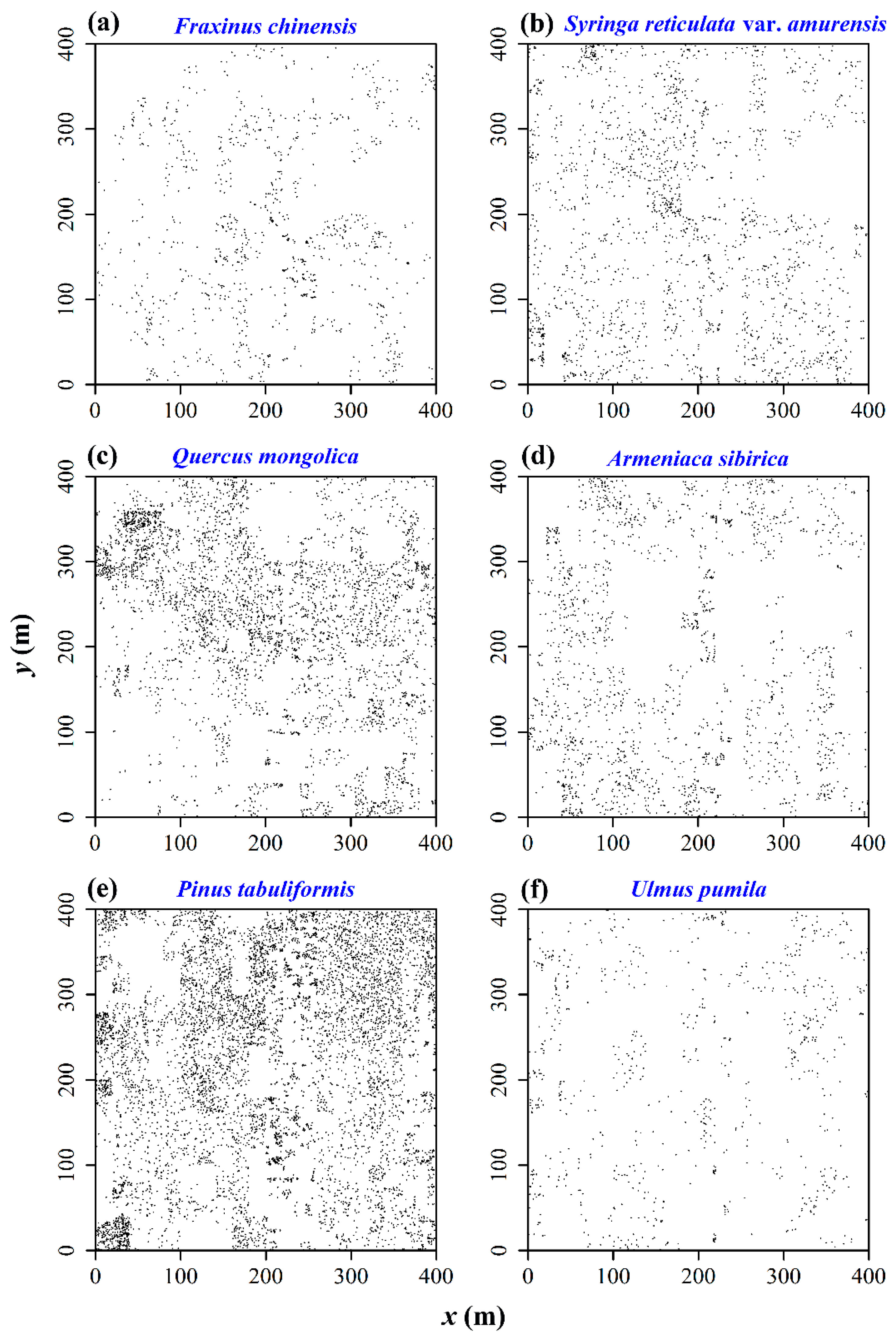
3.1. Abundances of Tree Species

Table 1. List of tree species in the study region [0, 400] × [0, 1000] (unit: m). y denotes the y-axis coordinate of the study region; NA denotes no value.

Species Code	Latin Name	Family	Abundance (0 ≤ y ≤ 1000 m)	Abundance (0 ≤ y ≤ 400 m)	Abundance (600 ≤ y ≤ 1000 m)	DBH (cm)	Height (m)
1	Acer mono Maxim.	Aceraceae	482	280	195	7.38 ± 4	5.9 ± 2.29
2	Acer truncatum Bunge	Aceraceae	228	124	92	7.66 ± 5.63	5.53 ± 3.08
3	Berberis beijingensis Ying	Berberidaceae	1	1	0	2.5 ± NA	1.75 ± NA
4	Betula dahurica Pall.	Betulaceae	205	138	62	13.92 ± 7.07	7.64 ± 3.12
5	Betula platyphylla Suk.	Betulaceae	89	42	46	17.43 ± 4.91	10.33 ± 1.7
6	Carpinus turczaninowii Hance	Betulaceae	8	1	4	7.65 ± 2.98	7.04 ± 1.05
7	Chimonanthus praecox (L.) Link	Calycanthaceae	3	3	0	5.47 ± 3.41	3.01 ± 0.37
8	Sambucus williamsii Hance	Caprifoliaceae	6	4	0	4.17 ± 0.94	2.56 ± 0.46
9	Diospyros lotus L.	Ebenaceae	2	0	0	20.83 ± 2.32	8.72 ± 0.49
10	Lithocarpus cleistocarpus (Seemen) Rehd. & E. H. Wils.	Fagaceae	19	15	4	5.38 ± 0.53	5.78 ± 0.6
11	Quercus mongolica Fisch. ex Ledeb.	Fagaceae	8466	4016	3064	11.07 ± 5.74	6.33 ± 2.73
12	Juglans cathayensis Dode	Juglandaceae	29	13	12	10.54 ± 10.66	8.1 ± 5.64
13	Juglans mandshurica Maxim.	Juglandaceae	824	376	211	11.84 ± 8.23	8.03 ± 3.9
14	Albizia kalkora (Roxb.) Prain	Leguminosae	156	93	59	6.98 ± 5.53	5.65 ± 2.94
15	Hibiscus mutabilis L.	Malvaceae	7	1	5	6.16 ± 0.73	6.16 ± 0.13
16	Myrtus communis L.	Myrtaceae	24	17	7	11.6 ± 0.6	7.52 ± 0.57
17	Fraxinus chinensis Roxb.	Oleaceae	1903	994	688	7.04 ± 4.26	5.27 ± 2.49
18	Fraxinus mandshurica Rupr.	Oleaceae	30	12	8	9.87 ± 6.81	7.85 ± 3.78
19	Fraxinus rhynchophylla Hance	Oleaceae	743	277	208	7.63 ± 4.87	5.6 ± 2.48
20	Syringa pekinensis Rupr.	Oleaceae	1	1	0	12.1 ± NA	7.35 ± NA
21	Syringa reticulata (Blume) H. Hara var. amurensis (Rupr.) J. S. Pringle	Oleaceae	4618	1935	1668	7.26 ± 4.35	5.27 ± 2.39
22	Pinus tabuliformis Carrière	Pinaceae Lindl.	24,579	7539	11,534	12.85 ± 6.02	8.55 ± 2.83
23	Rhamnus davurica Pall.	Rhamnaceae	2	0	1	7 ± 0.71	6.7 ± 0.14
24	Ziziphus jujuba Mill.	Rhamnaceae	62	18	37	11.1 ± 7.52	5.49 ± 2.97
25	Ziziphus jujuba Mill. var. spinosa (Bunge) Hu ex H. F. Chow	Rhamnaceae	3	0	2	14.63 ± 6.01	5.9 ± 2.72
26	Amygdalus davidiana (Carrière) de Vos ex Henry	Rosaceae	9	5	4	8.62 ± 4.26	6.65 ± 1.35
27	Armeniaca mume Sieb.	Rosaceae	4	4	0	4.98 ± 0.43	6.88 ± 0.16
28	Armeniaca sibirica (L.) Lam.	Rosaceae	6227	1789	2602	8.35 ± 4.55	5.04 ± 2.56
29	Crataegus pinnatifida Bunge	Rosaceae	1	0	0	10.5 ± NA	5.17 ± NA
30	Malus baccata (L.) Borkh.	Rosaceae	21	6	12	10.84 ± 12.52	4.96 ± 3.73
31	Prunus salicina Lindl.	Rosaceae	1	1	0	3.7 ± NA	2.8 ± NA
32	Pyrus bretschneideri Rehd.	Rosaceae	17	14	0	6.64 ± 0.75	4.32 ± 0.61
33	Sorbus alnifolia (Siebold & Zucc.) C. Koch	Rosaceae	121	18	42	8.73 ± 5.04	6.02 ± 2.66
34	Sorbus discolor (Maxim.) Maxim.	Rosaceae	492	71	168	7.71 ± 4.33	6.43 ± 2.46
35	Leptodermis potanini Batal.	Rubiaceae	220	19	62	4.82 ± 2.88	4.61 ± 1.84
36	Populus davidiana Dode	Salicaceae	37	23	11	9.97 ± 8.44	7.24 ± 2.94
37	Ailanthus altissima (Mill.) Swingle	Simaroubaceae	36	29	7	9.46 ± 7.68	7.71 ± 5.43
38	Tilia amurensis Rupr.	Tiliaceae	687	434	202	9.27 ± 4.87	6.76 ± 2.68
39	Tilia mandshurica Rupr. & Maxim.	Tiliaceae	2	0	2	12.35 ± 2.76	8.07 ± 2.22
40	Celtis bungeana Blume	Ulmaceae	655	403	181	5.61 ± 4.24	4.77 ± 2.39
41	Hemiptelea davidii (Hance) Planch.	Ulmaceae	12	0	1	6.71 ± 5.43	4.7 ± 2.53
42	Ulmus davidiana Planch. var. japonica (Rehder) Nakai	Ulmaceae	230	133	61	6.9 ± 4.42	5.78 ± 3.24
43	Ulmus macrocarpa Hance	Ulmaceae	133	5	31	7.71 ± 4.56	6.21 ± 2.33
44	Ulmus pumila L.	Ulmaceae	2124	826	729	12.79 ± 7.89	8.34 ± 3.66

provides the species name, the mean DBH, and heights with the corresponding standard deviations. There are six tree species that have high densities (1903 Fraxinus chinensis Roxb., 4618 Syringa reticulata (Blume) H. Hara var. amurensis (Rupr.) J. S. Pringle, 8466 Quercus mongolica Fisch. ex Ledeb., 6227 Armeniaca sibirica (L.) Lam., 24,579 P. tabuliformis, and 2124 Ulmus pumila L.), with Figure 1 illustrating the spatial distributions of these six dominant tree species in the subregion of [0, 400] × [0, 400] (unit: m).

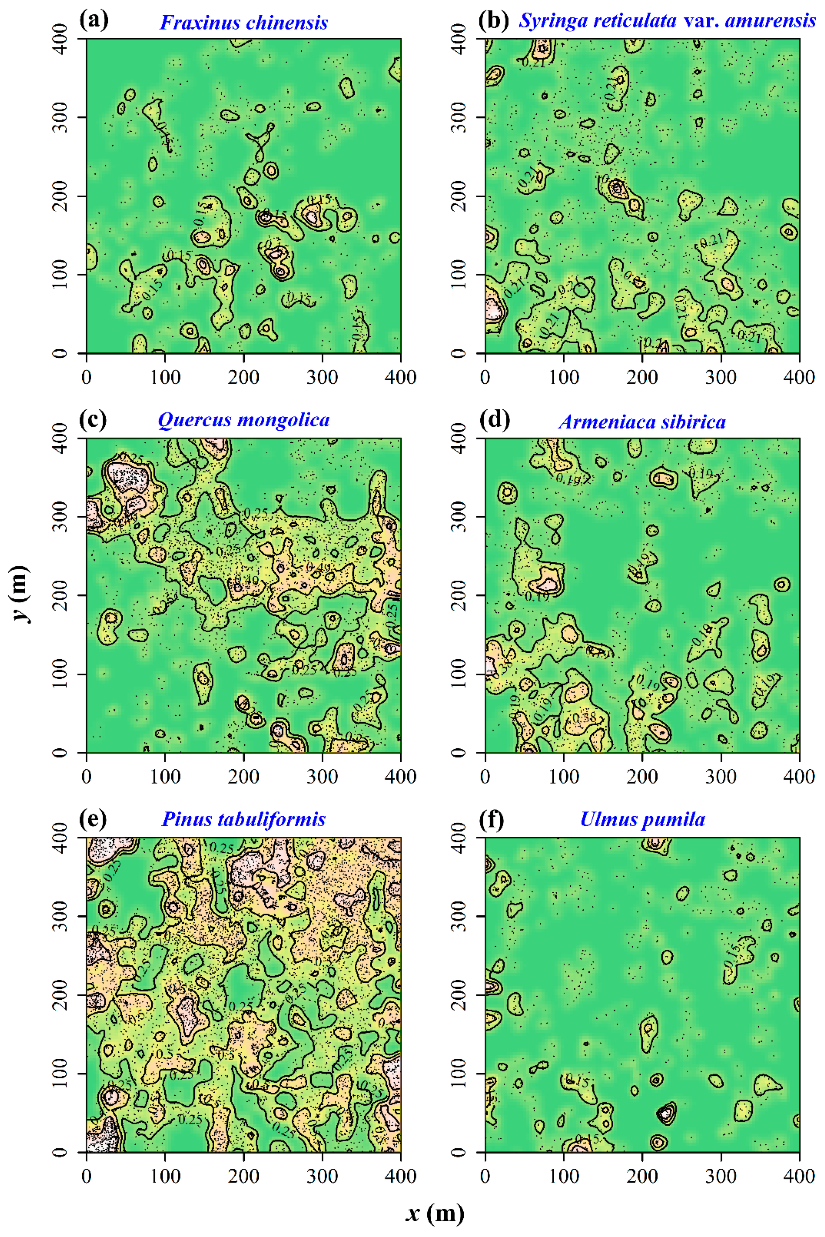
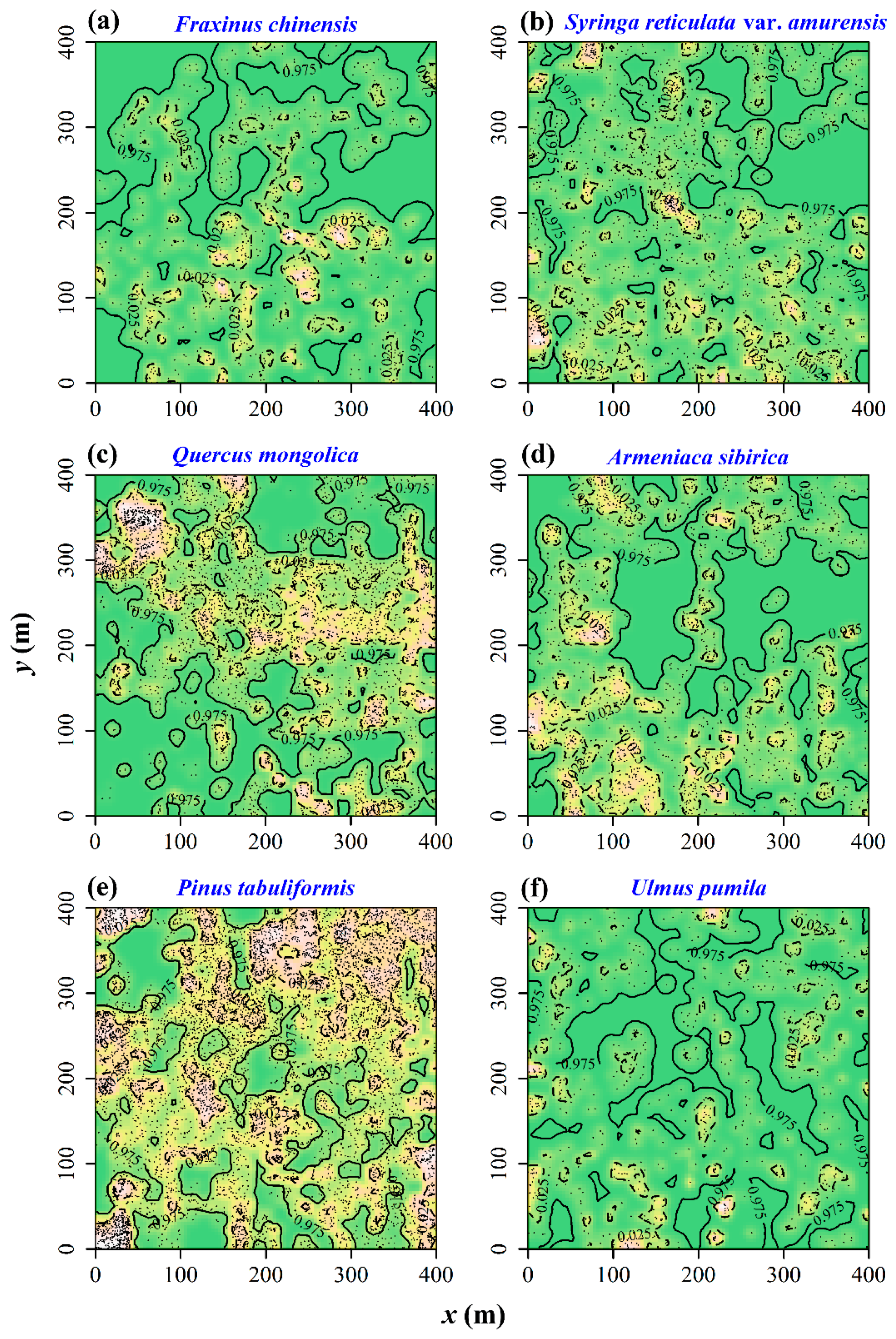
3.2. Test of Spatial Segregation

Figure 2 exhibits the bandwidth choice. When h = 5.5 m, the cross-validated log-likelihood was maximized. Figure 3 exhibits the species-specific probabilities of six dominant tree species in the region of [0, 400] × [0, 400] (unit: m). We can see that these tree species have occupied different subareas. The two most dominant tree species, Q. mongolica and P. tabuliformis, appeared to be spatially segregated. The overall p-value from the 399 Monte Carlo simulations, based on Equation (8) for testing spatial segregation, was 0.025, indicating significant spatial segregation for these six tree species. Figure 4 illustrates the 95% tolerance intervals on the p-value surfaces based on Equation (9), showing areas where the relative intensities are significantly higher/lower than the average based on the null hypothesis of no spatial segregation.

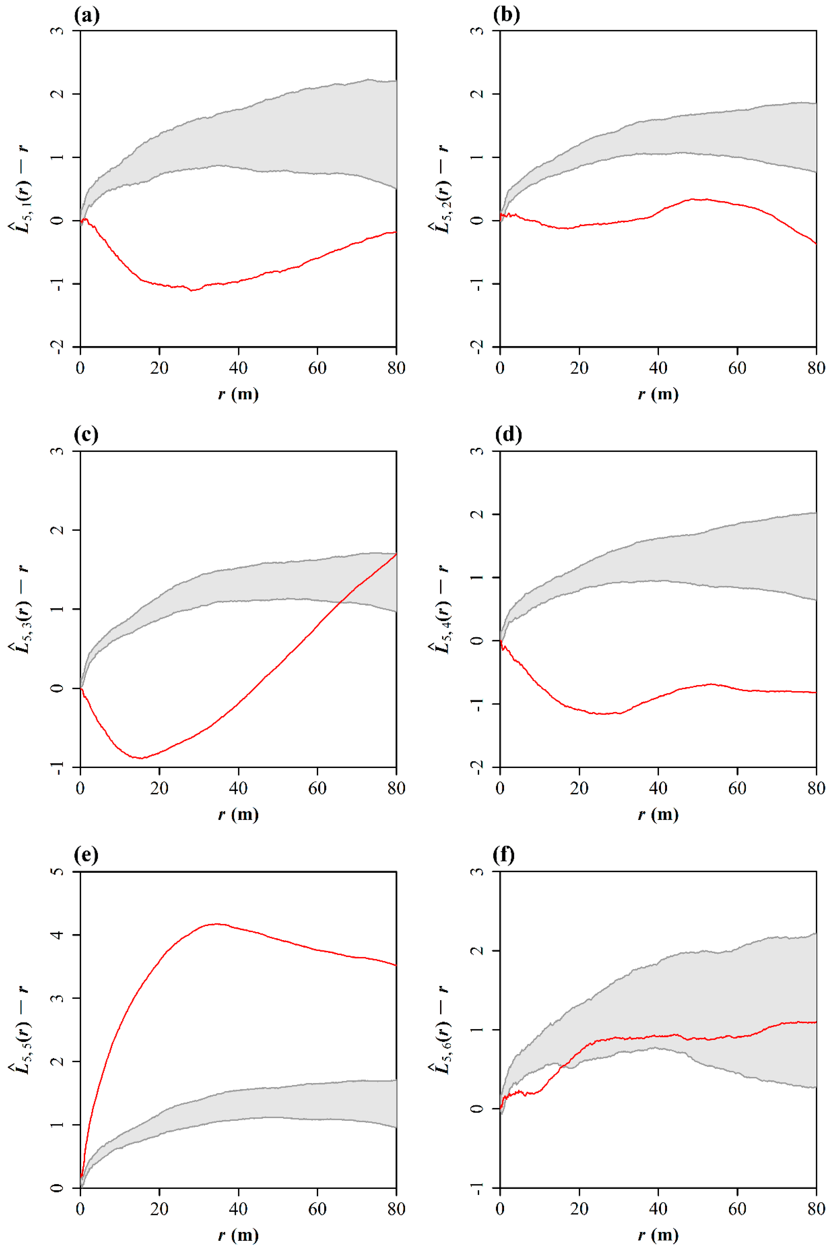
3.3. Spatial Correlations between the Chinese Pine and Other Five Tree Species

The cross-type L-function with the randomization test of the random labelling null hypothesis shows that there is significant relationship of repulsion between the Chinese pine and another four dominant species, with the exception of U. pumila (Figure 5). The estimates of ${\widehat{L}}_{12}\left(r\right)-r$ wandered outside the gray-shaded envelope. However, within 70 to 80 m scales, Q. mongolica and P. tabuliformis appear to be independent from each other (Figure 5c). On a scale from 0 to 20 m, U. pumila and P. tabuliformis have a repulsion relationship but, on larger scales, even up to 80 m, these two tree species show spatial independence. In addition, P. tabuliformis exhibits a spatial clustering in this study area, as the estimate also wandered outside the upper bound of envelope (Figure 5e).

For another study region of [0, 400] × [600, 1000] (unit: m), the results were the similar to the above results from the region of [0, 400] × [0, 400] (unit: m). The bandwidth for estimating the species-specific probabilities is 6 m, slightly higher than the estimate of bandwidth 5.5 m in the region of [0, 400] × [0, 400]. However, it does not affect the main results on spatial segregation (and, thus, is not shown).

4. Discussion

Ghalandarayeshi et al. [30] studied the spatial interactions of four dominant tree species in a semi-natural forest in Denmark (beech, elm, ash, and sycamore maple) based on cross-type g-function (i.e., the pair correlation function) which has the same function as the cross-type L-function for examining the spatial correlations between species [13]. They detected a weak repulsion relationship between beech and elm in less disturbed plots up to 6 m, and more disturbed plots up to 2 m. Over larger scales (up to 25 m), the two tree species appeared to intermingle in space. By contrast, beech and ash also intermingled in both less and more disturbed plots, indicating that these two species are distributed independently from each other. In disturbed plots, they detected spatial attraction between elm and ash up to 3 m apart, and between 8 to 12 m apart. Interestingly, they showed that these tree species did not exhibit spatial segregation in less disturbed plots. In another study, Xiang et al. [31] reported the spatial correlations among overstorey tree species, and between understorey trees and overstorey trees in a subtropical forest based on the cross-type L-function. They also found negative correlations (repulsion) among overstorey tree species. For the understory trees and overstorey trees that are less than 17 m apart, the two types of plants showed spatial independence (namely intermingled in space), although a repulsion relationship was detected for the two types of trees 17 and 40 m apart in space.

Although dominant tree species were found to have little negative correlations in the semi-natural forest of Denmark, we detected significant negative correlations between four species and the most dominant Chinese pine in our study. The site investigated by Ghalandarayeshi et al. [30] has been under conservation protection for a much longer period, and the forest community there might thus have experienced long-term natural succession, meaning that the dominant tree species at their report might have excluded other competitive tree species, or have reduced the densities of these competitive tree species to render them rare. In addition, greater spatial heterogeneity might be another factor that might explain the strong negative correlations between the Chinese pine and other four species in our study. Heterogeneous landscapes can result in spatial variations in competitive abilities among tree species, with weaker competitors (in homogeneous environments) potentially outcompeting stronger competitors with increasing environmental heterogeneity [32]. This also explains why, in the case of Xiang et al. [31], the species can coexist over large scales in the complex mountainous landscape, but still exhibit strong spatial competition.

Our study shows that the Chinese pines exhibits a spatial clustering (Figure 5e), although we did not distinguish the ages of trees. Although we found spatial segregation and spatial negative correlations among the six dominant tree species, there might be a lack of spatial negative correlations among the trees with different ages for the same species. Sandhu et al. [20] checked the spatial segregation of the moso bamboos with different ages using the method proposed by Diggle et al. [19], and they found that there was a significant spatial segregation among these moso bamboos. However, using the cross-type L-function to analyze the spatial correlations among these bamboos, we only detected spatial independence. The calculated ${\widehat{L}}_{12}\left(r\right)-r$ wandered inside the simulation envelopes. Also using the cross-type L-function, Wang et al. [33] explored the effect of gap size on the spatial patterns of Chinese pine regeneration, and found that the regeneration established before gap creation was independent from that after gap creation. This suggests that, for the same tree species, the trees with different ages do not show a tendency of repulsion or attraction. However, for the spatial point pattern, it was spatially aggregated on the scales from 0 to 5 m. By contrast, within 5−8 m, Chinese pines exhibited a Poisson random distribution [33]. Different from their results, our study shows that the Chinese pine population exhibited spatial clustering over the scale from 0 to 80 m, without any evidence for randomness. We think that the difference should be related to the extent of disturbance in the forests. In the study area of Wang et al. [33], although Chinese pine was still a dominant tree species, the grassland can also be temporarily dominant because of the excessive harvesting. By contrast, our study site was protected since 1985, with no harvesting allowed. Most natural pines have been intentionally kept when the reserve was established. After 30-year population recruitment, the present spatial distributions of Chinese pine could be more akin to its natural distribution and, thus, distributed in a spatial clustering way. In fact, spatial clustering is rather common for most plant species over large scales [12,34]. However, such a spatial clustering might only reflect the influence of environmental heterogeneity on the growth and dispersal of plants, e.g., following Matérn and Thomas processes [13,35].

Figure S1 in the online Supplementary Material shows the interspecific spatial correlation between P. tabuliformis and other five tree species obtained from the randomization test of the independence-of-components null hypothesis. The results appear to be unreliable because any other species exhibit a significant spatial independence from P. tabuliformis on almost all of the given distance scales, which is apparently not in accordance with the fact of interspecific competition, especially the root competition [36]. In the subregions that are dominantly occupied by P. tabuliformis, other tree species have a smaller chance to survive than those in the places where the population of P. tabuliformis has a lower density (Figure 1). We consider that the misuse of the independence of components as the null hypothesis of the randomization test might lead to a false conclusion. In mountainous areas, it is unsuitable to use the independence of components as the null hypothesis of a randomization test because of the spatial heterogeneity that exactly breaks down the precondition of using such a test [13]. The criticism of the use of the randomization test of the random labelling in analyzing the spatial correlations of different tree species focuses on the argument that the null hypothesis of applying this method is unsuitable because investigators are usually concerned about whether different tree species are spatially independent point processes. The null hypothesis of the randomization test of the random labelling is that the marks are conditionally independent and identically distributed [13,27]. However, the conditional independence is exactly what we want to know in examining whether weaker competitors are inclined to keep themselves far away from the sites where stronger competitors have occupied. Therefore, we advocate the use of the randomization test of the random labelling null hypothesis in exploring the spatial correlations of different tree species in heterogeneous environments. At least, the current study illustrates that the conclusions drawn from the non-parametric estimation of spatial segregation and those drawn from the cross-type L-function with the simulation envelopes generated by the random labelling were similar, whereas the randomization test with the independence-of-components null hypothesis provided unreliable results.

5. Conclusions

In our study area, F. chinensis, S. reticulate reticulata var. amurensis, Q. mongolica, A. sibirica, P. tabuliformis (Chinese pine), and U. pumila are dominant forest tree species. There are significant signs of spatial segregation between these six tree species. Although P. tabuliformis is the most dominant species, it does not drive other tree species to extinction, with each species dominating different subareas in the landscape, as shown in the surface of type(species)-specific probabilities. In particular, U. pumila had a positive spatial correlation with the Chinese pine over the scales from 20 to 80 m, whereas another four species had negative spatial correlations with the Chinese pine. This implies the possibility of species coexistence due, probably, to the spatial heterogeneity and disturbances in spite of notable interspecific competition between these species.

References

1. Wang, H.; Sork, V.L.; Wu, J.; Ge, J. Effect of patch size and isolation on mating patterns and seed production in an urban population of Chinese pine (Pinus tabuliformis Carr.). For. Ecol. Manag. 2010, 260, 965–974. [Google Scholar] [CrossRef]
2. Forman, R.T.T.; Godron, M. Patches and structural components for a landscape ecology. Bioscience 1981, 31, 733–740. [Google Scholar]
3. DeCesare, N.J.; Hebblewhite, M.; Robinson, H.S.; Musiani, M. Endangered, apparently: The role of apparent competition in endangered species conservation. Anim. Conserv. 2010, 13, 353–362. [Google Scholar] [CrossRef]
4. Hui, C.; Richardson, D.M. Invasion Dynamics; Oxford University Press: Oxford, UK, 2017. [Google Scholar]
5. Chu, C.; Kleinhesselink, A.R.; Havstad, K.M.; McClaran, M.P.; Peters, D.P.; Vermeire, L.T.; Wei, H.Y.; Adler, P.B. Direct effects dominate responses to climate perturbations in grassland plant communities. Nat. Commun. 2016, 7, 11766. [Google Scholar] [CrossRef] [PubMed] [Green Version]
6. Tilman, D.; Lehman, C.L.; Yin, C.J. Habitat destruction, dispersal, and deterministic extinction in competitive communities. Am. Nat. 1997, 149, 407–435. [Google Scholar] [CrossRef]
7. Lehman, C.L.; Tilman, D. Biodiversity, stability, and productivity in competitive communities. Am. Nat. 2000, 156, 534–552. [Google Scholar] [CrossRef]
8. Parry, G.D. The meanings of r- and K-selection. Oecologia 1981, 48, 260–264. [Google Scholar] [CrossRef]
9. Adler, P.B.; HilleRisLambers, J.; Levine, J.M. A niche for neutrality. Ecol. Lett. 2007, 10, 95–104. [Google Scholar] [CrossRef]
10. Chesson, P. General theory of competitive coexistence in spatially-varying environments. Theor. Popul. Biol. 2000, 58, 211–237. [Google Scholar] [CrossRef]
11. Connell, J.H. On the role of natural enemies in preventing competitive exclusion in some marine animals and in rain forest trees. Dyn. Popul. 1971, 298, 298–312. [Google Scholar]
12. Diggle, P.J. Statistical Analysis of Spatial and Spatio-temporal Point Patterns; CRC Press: London, UK, 2014. [Google Scholar]
13. Baddeley, A.; Rubak, E.; Turner, R. Spatial Point Patterns: Methodology and Applications with R; Chapman & Hall/CRC: London, UK, 2015. [Google Scholar]
14. Hui, C.; Landi, P.; Minoarivelo, H.O.; Ramanantoanina, A. Ecological and Evolutionary Modelling; Springer: Cham, Switzerland, 2018. [Google Scholar]
15. Baddeley, A.; Diggle, P.J.; Hardegen, A.; Lawrence, T.; Milne, R.K.; Nair, G. On tests of spatial pattern based on simulation envelopes. Ecol. Monogr. 2014, 84, 477–489. [Google Scholar] [CrossRef]
16. Ripley, B.D. Modelling spatial patterns (with discussion). J. R. Stat. Soc. B 1977, 39, 172–212. [Google Scholar]
17. Hui, C.; Veldtman, R.; McGeoch, M.A. Measures, perceptions and scaling patterns of aggregated species distributions. Ecography 2010, 33, 95–102. [Google Scholar] [CrossRef]
18. Hui, C.; Vermeulen, W.; Durrheim, G. Quantifying multiple-site compositional turnover in an Afrotemperate forest, using zeta diversity. For. Ecosyst. 2018, 5, 15. [Google Scholar] [CrossRef] [Green Version]
19. Diggle, P.; Zheng, P.P.; Durr, P. Nonparametric estimation of spatial segregation in a multivariate point process: Bovine tuberculosis in Cornwall, UK. J. R. Stat. Soc. Ser. C Appl. Stat. 2005, 54, 645–658. [Google Scholar] [CrossRef]
20. Sandhu, H.S.; Shi, P.; Yang, Q. Intraspecific spatial niche differentiation: Evidence from Phyllostachys edulis. Acta Ecol. Sin. 2013, 33, 287–292. [Google Scholar] [CrossRef]
21. Serra, L.; Juan, P.; Varga, D.; Mateu, J.; Saez, M. Spatial pattern modelling of wildfires in Catalonia, Spain 2004–2008. Environ. Model. Softw. 2013, 40, 235–244. [Google Scholar] [CrossRef] [Green Version]
22. Lu, Z.B.; Shi, P.J.; Reddy, G.V.P.; Li, L.M.; Men, X.Y.; Ge, F. Nonparametric estimation of interspecific spatio-temporal niche separation between two lady beetles (Coleoptera: Coccinellidae) in Bt cotton fields. Ann. Entomol. Soc. Am. 2015, 108, 807–813. [Google Scholar] [CrossRef]
23. Sun, J.; Liu, Y. Age-independent climate-growth response of Chinese pine (Pinus tabuliformis Carrière) in North China. Trees Struc. Funct. 2015, 29, 397–406. [Google Scholar] [CrossRef]
24. Liu, Y.; Liu, H.; Song, H.; Li, Q.; Burr, G.S.; Wang, L.; Hu, S. A monsoon-related 174-year relative humidity record from tree-ring in δ18O the Yaoshan region, eastern central China. Sci. Total Environ. 2017, 593−594, 523–534. [Google Scholar] [CrossRef]
25. Kelsall, J.E.; Diggle, P.J. Spatial variation in risk of disease: A nonparametric binary regression approach. Appl. Stat. 1998, 47, 559–573. [Google Scholar] [CrossRef]
26. Hui, C.; McGeoch, M.A.; Warren, M. A spatially explicit approach to estimating species occupancy and spatial correlation. J. Anim. Ecol. 2006, 75, 140–147. [Google Scholar] [CrossRef] [PubMed] [Green Version]
27. Goreaud, F.; Pélissier, R. Avoiding misinterpretation of biotic interactions with the intertype K12-function: Population independence vs. random labelling hypotheses. J. Veg. Sci. 2003, 14, 681–692. [Google Scholar] [CrossRef]
28. Grabarnik, P.; Myllymäki, M.; Stoyan, D. Correct testing of mark independence for marked point patterns. Ecol. Model. 2011, 222, 3888–3894. [Google Scholar] [CrossRef]
29. R Core Team. R: A Language and Environment for Statistical Computing; R Foundation for Statistical Computing: Vienna, Austria, 2015; Available online: https://www.R.-project.org (accessed on 17 April 2018).
30. Ghalandarayeshi, S.; Nord-Larsen, T.; Johannsen, V.K.; Larsen, J.B. Spatial patterns of tree species in Suserup Skov—A semi-natural forest in Denmark. For. Ecol. Manag. 2017, 406, 391–401. [Google Scholar] [CrossRef]
31. Xiang, W.; Liu, S.; Lei, X.; Frank, S.C.; Tian, D.; Wang, G.; Deng, X. Secondary forest floristic composition, structure, and spatial pattern in subtropical China. J. For. Res. 2013, 18, 111–120. [Google Scholar] [CrossRef]
32. Legendre, P.; Fortin, M.-J. Spatial pattern and ecological analysis. Plant Ecol. 1989, 80, 107–138. [Google Scholar] [CrossRef] [Green Version]
33. Wang, Z.; Yang, H.; Dong, B.; Zhou, M.; Ma, L.; Jia, Z.; Duan, J. Effects of canopy gap size on growth and spatial patterns of Chinese pine (Pinus tabuliformis) regeneration. For. Ecol. Manag. 2017, 385, 46–56. [Google Scholar] [CrossRef]
34. Diggle, P.J.; Gómez-Rubio, V.; Brown, P.E.; Chetwynd, A.G.; Gooding, S. Second-order analysis of inhomogeneous spatial point processes using case–control data. Biometrics 2007, 63, 550–557. [Google Scholar] [CrossRef]
35. Shi, P.J.; Sandhu, H.S.; Reddy, G.V.P. Dispersal distance determines the exponent of the spatial Taylor’s power law. Ecol. Model. 2016, 335, 48–53. [Google Scholar] [CrossRef]
36. Hou, H.; Ding, L.; Xu, Z.; Wang, L.; Zhao, Y. Root distribution of young trees of typical species in the northern region of Yanshan Mountains. For. Resour. Manag. 2018, 10–15. (In Chinese) [Google Scholar]
Figure 1. Spatial distributions of six dominant tree species in the study region of [0, 400] × [0, 400] (unit: m). (a) F. chinensis; (b) S. reticulata var. amurensis; (c) Q. mongolica; (d) A. sibirica; (e) P. tabuliformis; (f) U. pumila.
Forests 09 00768 g001
Figure 2. Cross-validated log-likelihood for the six dominant tree species. The grey curve represents the cross-validated log-likelihood values corresponding to different candidate bandwidths (h). The cross-validated log-likelihood associated with h = 5.5 m is maximal (see the red point at which the grey curve and the blue vertical dashed line intersect).
Forests 09 00768 g002
Figure 3. The type-specific probabilities of six dominant tree species. In each panel, the brighter the color is, the higher the type-specific probability is. There are some isolines of the type-specific probabilities. (a) F. chinensis; (b) S. reticulata var. amurensis; (c) Q. mongolica; (d) A. sibirica; (e) P. tabuliformis; (f) U. pumila.
Forests 09 00768 g003
Figure 4. The p-value surfaces for six dominant tree species based on 399 Monte Carlo simulations. In each panel, the brighter the color is, the higher the p-value is. There are two isolines: 0.025 and 0.975. The areas with the p-value less than 0.025 have greater relative intensities than the average level, and the areas with the p-value greater than 0.975 have lower relative intensities than the average level. (a) F. chinensis; (b) S. reticulata var. amurensis; (c) Q. mongolica; (d) A. sibirica; (e) P. tabuliformis; (f) U. pumila.
Forests 09 00768 g004
Figure 5. Analysis of spatial relationship between Chinese pine and five other tree species based on the randomization test of the random labelling null hypothesis. In the subscript of the estimated cross-type L, 1 represents F. chinensis, 2 represents S. reticulata var. amurensis, 3 represents Q. mongolica, 4 represents A. sibirica, 5 represents P. tabuliformis, and 6 represents U. pumila. The grey area are formed by simulation envelops; the red curve represents the difference between the estimated cross-type L of two types minus the corresponding distance scale r. (a) P. tabuliformis and F. chinensis; (b) P. tabuliformis and S. reticulata var. amurensis; (c) P. tabuliformis and Q. mongolica; (d) P. tabuliformis and A. sibirica; (e) P. tabuliformis and itself; (f) P. tabuliformis and U. pumila.
Forests 09 00768 g005