Article

Tree-Lists Estimation for Chinese Boreal Forests by Integrating Weibull Diameter Distributions with MODIS-Based Forest Attributes from kNN Imputation

1
CAS Key Laboratory of Forest Ecology and Management, Institute of Applied Ecology, Shenyang 110016, China
2
School of Civil and Architectural Engineering, Shandong University of Technology, Zibo 255049, China
3
School of Natural Resources, University of Missouri, 203 Anheuser-Busch Natural Resources Building, Columbia, MO 65211, USA
4
School of Geographical Sciences, Northeast Normal University, Changchun 130024, China
*
Author to whom correspondence should be addressed.
Forests 2018, 9(12), 758; https://doi.org/10.3390/f9120758
Submission received: 16 October 2018 / Revised: 24 November 2018 / Accepted: 30 November 2018 / Published: 5 December 2018

Abstract

:
Wall-to-wall tree-lists information (lists of species and diameter for every tree) at a regional scale is required for managers to assess forest sustainability and design effective forest management strategies. Currently, the k-nearest neighbors (kNN) method and the Weibull diameter distribution function have been widely used for estimating tree lists. However, the kNN method usually relies on a large number of field inventory plots to impute tree lists, whereas the Weibull function relies on strong correlations between stand attributes and diameter distribution across large regions. In this study, we developed a framework to estimate wall-to-wall tree lists over large areas based on a limited number of forest inventory plots. This framework integrates the ability of extrapolating diameter distribution from Weibull and kNN imputation of wall-to-wall forest stand attributes from Moderate Resolution Imaging Spectroradiometer (MODIS). We estimated tree lists using this framework in Chinese boreal forests (Great Xing’an Mountains) and evaluated the accuracy of this framework. The results showed that the passing rate of the Kolmogorov–Smirnov (KS) test for Weibull diameter distribution by species was from 52% to 88.16%, which means that Weibull distribution could describe the diameter distribution by species well. The imputed stand attributes (diameter at breast height (DBH), height, and age) from the kNN method showed comparable accuracy with the previous studies for all species. There was no significant difference in the tree density between the estimated and observed tree-lists. Results suggest that this framework is well-suited to estimating the tree-lists in a large area. Our results were also ecologically realistic, capturing dominant ecological patterns and processes.

1. Introduction

Tree-lists (i.e., lists of species and diameter for every tree) [1] are of primary importance for deriving many stand attributes of interest (e.g., species composition, basal area, biomass). They are also valuable information for parameterizing forest landscape models (FLMs) [2], which are useful tools to examine how climate change, forest management, and other environmental stressors interact with species distributions and ecosystem conditions over large areas and long time frames [3,4]. As such, tree-lists across large regions are required to assess forest sustainability and design effective forest management strategies in response to various disturbance regimes for forest managers and researchers [2,3,4].
Tree-lists data are often obtained through field inventories [5], which record the species and diameter of every tree in the plot. However, field inventories are labor-intensive and unfeasible for large areas [1,6]. Therefore, researchers usually integrate forest inventory data, remotely sensed data, and environment data to extrapolate tree-lists to a large area based on the limited plots [7,8,9,10,11,12]. Generally, there are two extrapolation approaches: imputation methods and parametric diameter distribution modeling [10,13].
Imputation methods involve a series of nonparametric statistical methods such as k-nearest neighbors (kNN) [14], most similar neighbors [15], random forests [16], and geo-statistical estimation [17] to fill target units with measurements from one (or several) reference unit(s) in the population [1,18]. Particularly, the kNN imputation method is widely used for estimating tree-lists. When using kNN imputation, the target units are assigned with the tree-lists of the reference units from field inventory based on the similarity between the reference and target stands [1,8]. The major advantage of the kNN imputation method is the preservation of the covariance structure of the tree-lists from the reference data, and it is suitable for modeling multi-model diameter distribution for complex stands [1,15]. However, kNN imputation is particularly vulnerable for extrapolations beyond the range of the sample [19]. Therefore, a large number of field plots with tree-lists are required when using kNN imputation over large areas. This may present a problem in some regions due to data rights and data scarcity.
The other extrapolation method—parametric diameter distribution modeling—uses parametric distribution functions such as the log-normal, exponential, gamma, beta, Johnson's SB, and Weibull functions to fit the diameter distribution for each stand, and then estimates the stand attributes that correlate to the distribution parameters [1,20]. Once the parameters of the distribution are determined, the proportions of tree number at each diameter class are identified by the theoretical diameter distributions. Compared to the kNN method, these methods are not limited by the attribute range of training sample data, and extrapolation is generally possible if parametric diameter distribution models are calibrated properly [10,13]. The Weibull function is the best parametric function for diameter distribution because it has fewer parameters to be estimated and flexibility in describing different shapes of diameter distributions for many tree species worldwide [10,20,21]. Generally, the Weibull parameters can be estimated by building the relationships between the Weibull parameters and stand attributes (e.g., stand age, mean height, mean diameter, and aboveground biomass (AGB) density). Such stand attributes can be obtained from lidar data or high spatial resolution optical images [1,22,23,24]. Therefore, lidar or high spatial resolution optical images are often used in multi-phase sampling procedures to obtain stand attributes in lieu of field plots in large regions [22,23]. However, the wall-to-wall coverage of these stand attributes is also lacking across large regions due to the high cost of acquiring and processing lidar data or other spatial optical images. The application of Weibull diameter distribution across large regions is also limited by the validity of the stand attributes that are assumed to have strong correlations to the parameters of the Weibull diameter distribution.
To combine the strengths of kNN and Weibull methods for wall-to-wall stand attributes imputation across large regions, it is possible to integrate Weibull parameters estimated from field plots with the stand attributes imputed from kNN [25]. Therefore, our objective in this study was to develop a framework to estimate tree-lists based on limited forest inventory tree-lists data by integrating a parametric Weibull density function with stand attributes imputed by the kNN method. We further tested and assessed this framework and estimated wall-to-wall tree-lists at 250 m spatial resolution in the boreal forests of China. Our study provides a practical approach to estimating tree-lists over large areas where open-source forest inventory data are lacking.

2. Materials and Methods

2.1. Study Area

Our study area was located in the Great Xing’an Mountains in China, which is a typical southern boreal forest area with elevations varying from 139 to 1511 m (121°12′–127°00′ E, 50°10′–53°33′ N) (Figure 1). This area has a cold temperate continental monsoon climate with average annual temperature varying from 1 °C at its southern extremes to −6 °C at its northern extremes, and precipitation varying from 442 mm in the south to 240 mm in the north. More than 60% of the annual precipitation falls in the summer season from June to August [26]. The slope of our study area is relatively gentle, with 80% of the area less than 15°. Most of the landscape is mainly dominated by cool temperate coniferous forests. The main boreal conifer tree species is Dahurian larch (Larix gmelinii (Rupr.) Kuzen, hereafter “larch”), which are usually found in cool moist sites. The broadleaf tree species mainly include white birch (Betula platyphylla Suk.) and aspen (Populus davidiana Dode), and occupy drier, well-drained sites of the area [27]. Other tree species, such as Korean spruce (Picea koraiensis Nakai, hereafter “spruce”), Asian black birch (Betula davurica Pall., hereafter “black birch”), Mongolian Scots pine (Pinus sylvestris var. mongolica Litv., hereafter “pine”), willow (Chosenia arbutifolia (Pall.) A. Skv.), Mongolian oak (Quercus mongolica Fisch. ex Ledeb.), and a shrub species (Pinus pumila (Pall.) Regel), are interspersed with larch forests and have a small area of distribution [28]. Black birch and Mongolian oak were mainly distributed in the southern part of the study area, whereas pine was distributed in the northern part. Young and middle-aged forests comprised the main part of the forest landscapes, with the exception of the conservation area due to long-term logging and fire disturbance. The forest structures varied due to frequent disturbance and large spatial variation in climate and terrain.

2.2. Plot and Stand Inventory Data

Two types of forest inventory data were collected in this study. One was the limited plot inventory data with tree-lists, which were used to build the parameter estimation models of Weibull diameter distributions by species. The other were the stand inventory data without tree-lists, which were used to estimate the wall-to-wall stand attributes by the kNN imputation method.
The plot inventory data included a total of 212 plots, which were measured in Huzhong and Jiagedaqi forestry bureaus in 2011 (Figure 1). Among these plots, 191 plots were in the middle part of the study area and contained most tree species of the study area except Mongolian oak and black birch. Thus, we surveyed another 21 plots that included Mongolian oak and black birch located in the southern part of the study area. All plots were 20 m × 30 m. The diameter at breast height (DBH) for all trees larger than 5 cm was measured in each plot. We also recorded the GPS coordinates, slope, elevation, mean stand age, and mean height in each plot. We calculated the arithmetic mean DBH by species by dividing the sum of tree DBHs by the tree number of corresponding tree species.
Stand inventory data were collected from the China Forestry Science Data Center (CFSDC, http://www.cfsdc.org), which included 7635 stand polygons with relatively complete attributes from 1997 to 2001. These stand polygons ranged from a few hectares to dozens of hectares. Within each stand polygon, stand characteristics such as stand DBH, height, age, tree species composition (volume proportion), and the stand volume density were recorded in accordance with Chinese inventory requirements for forest management planning and design [29]. Stand DBH is the DBH of the trees with the mean basal area of the stand. It is different from mean arithmetic mean DBH. The detailed information about polygon stand inventory data can be found in Zhang et al. [30].

2.3. Predictor Variables

Forest stand characteristics can be characterized by the reflectance values of satellite images and influenced by environment factors. In this study, Moderate Resolution Imaging Spectroradiometer (MODIS) satellite image variables and environment variables were selected as predictor variables to estimate wall-to-wall stand attributes (e.g., stand mean DBH, height, and age). The detailed lists of predictor variables can be found in Zhang et al. [30]. MODIS variables included seven MODIS monthly composite surface reflectance bands and several vegetation indices correlated with vegetation characteristics in June of 2000. Environment variables in this study included climate variables, topographic variables, and location variables. Climate variables included mean annual precipitation and temperature between 1982 and 2009, (raster layers with a 1 km spatial resolution), which were generated by interpolating data from the National Meteorological Center of China by Mao et al. [31]. Topographic variables including elevation, slope, and cosine of aspect (COSASP) were derived from the Shuttle Radar Topography Mission digital elevation model (SRTMDEM, 90 m spatial resolution). SRTMDEM was downloaded from the International Scientific and Technical Data Mirror Site, Computer Network Information Center, Chinese Academy of Sciences (http://www.gscloud.cn/). All the predictor variables except for topographic variables were resampled to 250 m pixel resolution using nearest neighbor method.

2.4. Overall Framework for Tree-Lists Estimation

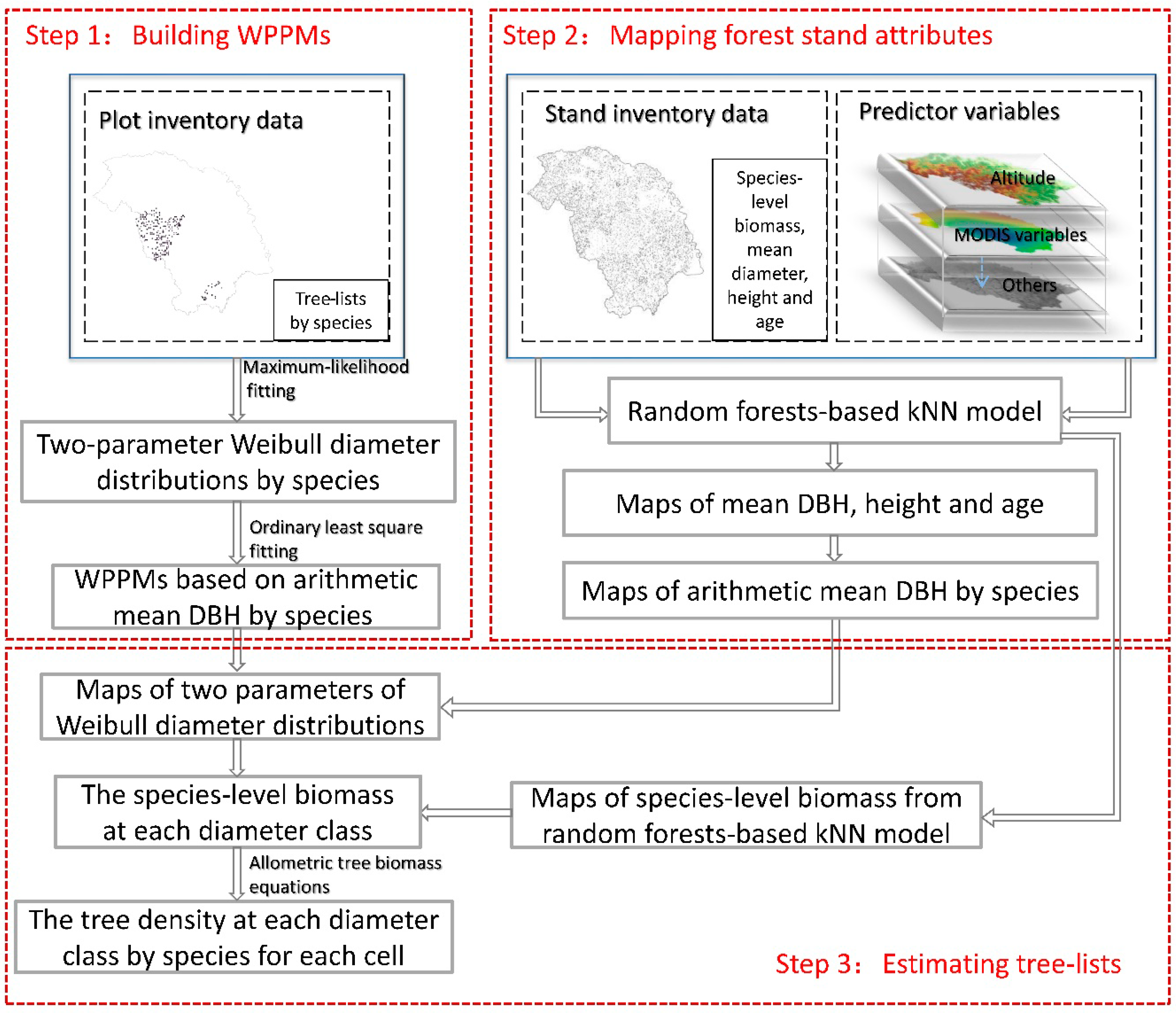
The approach in this study included the following steps (Figure 2): (1) We built the Weibull parameter prediction models (WPPMs) using plot inventory data for estimating diameter distributions in each pixel; (2) We used kNN models to map forest stand attributes (e.g., species-level biomass, stand age, height, DBH) and provided the independent variables for WPPMs in each pixel; (3) We estimated tree-lists by species in each pixel by combining Weibull diameter distributions estimated by WPPMs and forest stand attributes imputed by the kNN method.

2.4.1. Building WPPMs

The two-parameter Weibull function was applied to modeling the diameter distribution by species in the 212 plots. The equation of the Weibull probability density function is
f ( x ) = b c ( x c ) b 1 exp [ ( x c ) b ]
where f(x) is the tree density probability function with diameter, x represents diameter, and b and c are the shape parameter and scale parameter of the function, respectively.
Maximum likelihood estimation (MLE, Equation (2)) was used to estimate the parameters of the Weibull functions of each species for each plot. MLE is a common method used to estimate the parameters of distributions [20,21]. The MLE equation is as follows:
L ( x 1 ,   x 2 , , x n , θ ) = i = 1 n f ( x i , θ )
where x1, x2, , xn are the observed values of the samples from the population, L ( x 1 ,   x 2 , , x n ,   θ ) is the MLE function, and f ( x ,   θ ) is the probability density function with unknown parameters ( θ ). The maximum probability for the samples (x1, x2, , xn) is required when using MLE method to estimate the value of θ . If the MLE function (L) is a differentiable function, the value of θ satisfies the requirement of the function:
d L d θ = 0
According to Equation (3), the unknown parameters can be estimated. The MLE method was executed using the MASS package [32] in R [33]. When parameters b and c were estimated in each plot, the relationship between the parameters and stand variables could be built. In this study, arithmetic mean DBH by species was selected as the independent variable to build WPPMs using the ordinary least squares (OLS) method.

2.4.2. Mapping Forest Stand Attributes

The stand attributes including DBH, age, and height were mapped by integrating the forest attributes from stand polygons with predictor variables as described in Section 2.3 using the kNN method. The inverse distance weighted method and k = 6 that Zhang et al. used were selected to weight the nearest neighbor reference elements. The mean arithmetic DBH for larch and white birch in each pixel were separately estimated using mean stand DBH, age, and height as independent variables by Equations (4) and (5), which were built by Qi [34]:
L D = e 0.25412 + 1.064046 l n D + 0.002369 t 0.0074 H ,
B D = e 0.393344 + 0.831571 l n D + 0.00305 t + 0.005589 H .
LD is the mean arithmetic DBH of larch, BD is the mean arithmetic DBH of white birch, D is mean stand DBH, t is the stand age, and H is the mean stand height. For other species, we used mean stand DBH instead of mean arithmetic DBH as the independent variable to estimate the diameter distribution in each pixel. When mean arithmetic DBH by species was estimated, parameters b and c of the Weibull function by species in each pixel could be calculated using the WPPMs.

2.4.3. Generating Tree-Lists by Species

Species-level biomass in step two for the study area in 2000 were from a previous study, from which the accuracy for the species-level biomass assessment was provided [30]. In step three, the species-level biomass was used to estimate the tree-lists in each pixel with the diameter distribution by species. Once diameter distribution by species was estimated by WPPMs in each pixel, the proportion of the tree density at each diameter class by species (PTDS) could be calculated in each pixel. Then, the proportion of the species-level biomass at each diameter class (PSB) was calculated according to PTDS and single-tree biomass by species at each diameter class [35]. Finally, the species-level biomass could be divided into each diameter class according to the PSB and converted to the tree density at each diameter class by dividing them by the single tree biomass at each diameter class.

2.5. Accuracy Assessment

In order for our framework to have a reliable accuracy, each step of the method was assessed using a variety of accuracy measures.
In the first step, the goodness of fit of the estimated Weibull diameter distributions in each plot was evaluated by the Kolmogorov–Smirnov (KS) test [36,37] and an error index proposed by Packalén and Maltamo [12]:
e = i = 1 k 0.5 | f i N f i ˇ N ˇ | ,
where f i is the observed stem number of class i by species, f i ˇ is the estimated stem number of class i by species based on WPPMs, N is the total observed stem number by species, and N ˇ is the total estimated stem number by species. The error index ranges from 0 to 1, with 0 meaning a perfect fit and 1 meaning that the distributions do not overlap at all [38].
WPPMs were evaluated by using leave-one-out cross-validation (LOOCV). The R2, root mean square error (RMSE), and bias were calculated based on the parameters of Weibull diameter distribution functions:
RMSE = i = 1 n ( y i y ˇ i ) n ,
R 2 = 1 i = 1 n ( y i y i ˇ ) 2 / i = 1 n ( y i y ¯ ) 2 ,
Bias = i = 1 n ( y i y ˇ i ) n ,
where n is the number of the samples, y i is the ith observed value, y i ˇ is the ith estimated value, and y ¯ is the mean value of all the observed values. For assessment of WPPMs’ accuracy, n is the number of plots used to fit WPPMs for each species, y i is the parameter value estimated for plot i based on MLE, and y i ˇ is the parameter value estimated for plot i based on WPPMs.
Because R2, root mean square error (RMSE), and bias have also been widely used to evaluate the accuracy of many maps of forest stand attributes, the maps of stand attributes (e.g., stand DBH, height, and age) in the second step were also evaluated by calculating these three measures using stand inventory polygons from the CFSDC. Although all stand inventory polygons were used in random forests-based kNN (RF-kNN) model development, only the 2nd through 7th nearest-neighboring polygons were used to impute stand attributes for each target pixel. This means that each polygon was not used to impute the pixels that had the same place as it and only contributed minimally to the estimate for the corresponding pixel. Thus, the two datasets can be deemed independent for comparisons between the field stand values and the modeled pixel values with the same spatial place.
Assessments for estimated tree-lists by species in the year 2000 across the study area were difficult because we only had the inventory tree-lists data in 2011. In order to compare with the estimated tree-lists of 2000, we transformed the inventory tree-lists data of 2011 by subtracting the DBH growth of the six species in the past eleven years based on equations (Table 1) which were built using the ordinary least squares (OLS) method and evaluated using the leave-one-out cross validation (LOOCV) method against the published data [39]. We evaluated the accuracy of the estimated tree-lists in 2000 by calculating the error index based on these transformed inventory tree-lists data. The error indices by species were calculated by each plot and by all the plots as a whole.
We also divided the forest inventory data in 2011 into three age classes (Young, Middle, and Mature) by technical regulations for inventory for forest management planning and design (GB/T26424-2010). Additionally, we compared the tree density from observed tree-lists data in 2011 with that derived from estimated tree-lists data in 2000 for the three main forest types (i.e., larch forests, white birch forests, and mixed forests) with the same age class and similar environment using analysis of variance (ANOVA). When identifying the similar environment, we mainly considered three factors: slope, aspect, and elevation.

3. Results

3.1. Weibull Parameter Prediction Models

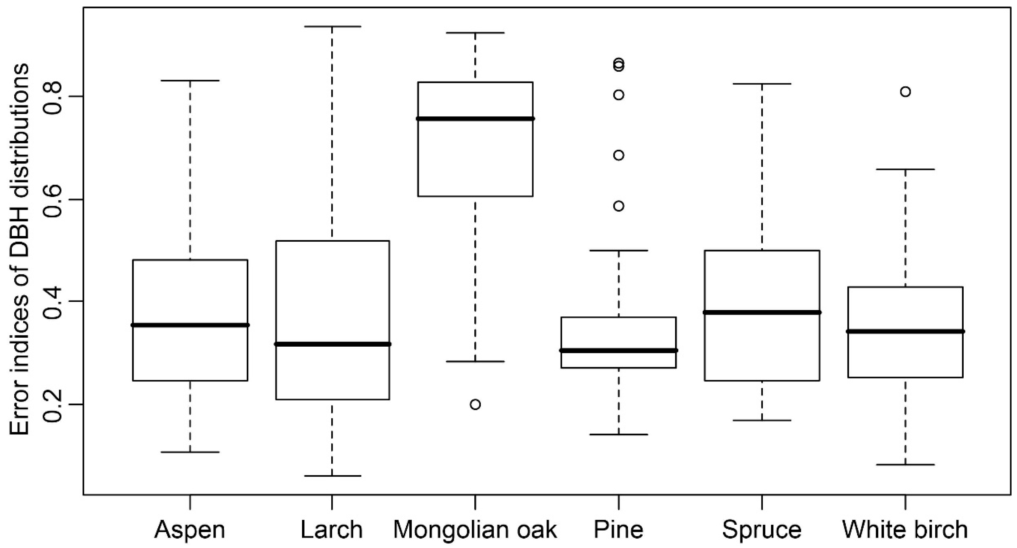
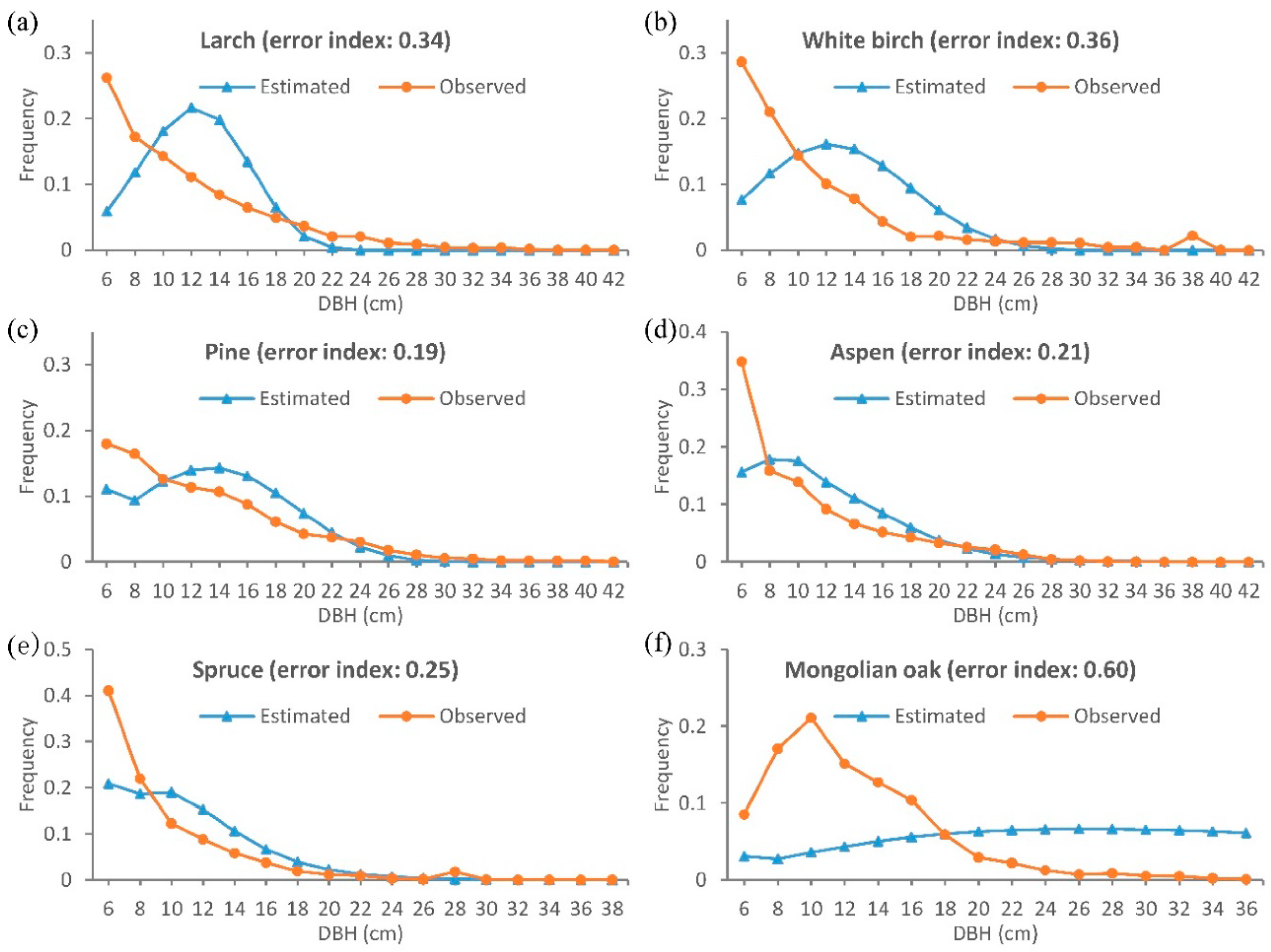
The KS test showed that diameter distributions of all species could be well fitted using the Weibull functions estimated by the MLE method (agreement > 50%), especially for larch, white birch, and pine (Table 2, agreement > 80%). The leave-one-out cross validation (LOOCV) of WPPMs showed that the scale parameter (c) had a good relationship with the arithmetic mean DBH (d) for all the species (Table 3, small RMSE and high R2). However, the arithmetic mean DBH (d) explained less variation in shape parameter (b) among different plots (R2: 0.13–0.29). Overall, diameter distributions by species in each plot were well-fitted, with mean values of error indices from 0.27 to 0.43, except for Mongolian oak. When separately summing the estimated and observed trees by diameter class of species to calculate the error indices, all the species diameter distributions were well-represented with low error indices (0.04–0.14) (Table 4).

3.2. Maps of Forest Stand Attributes

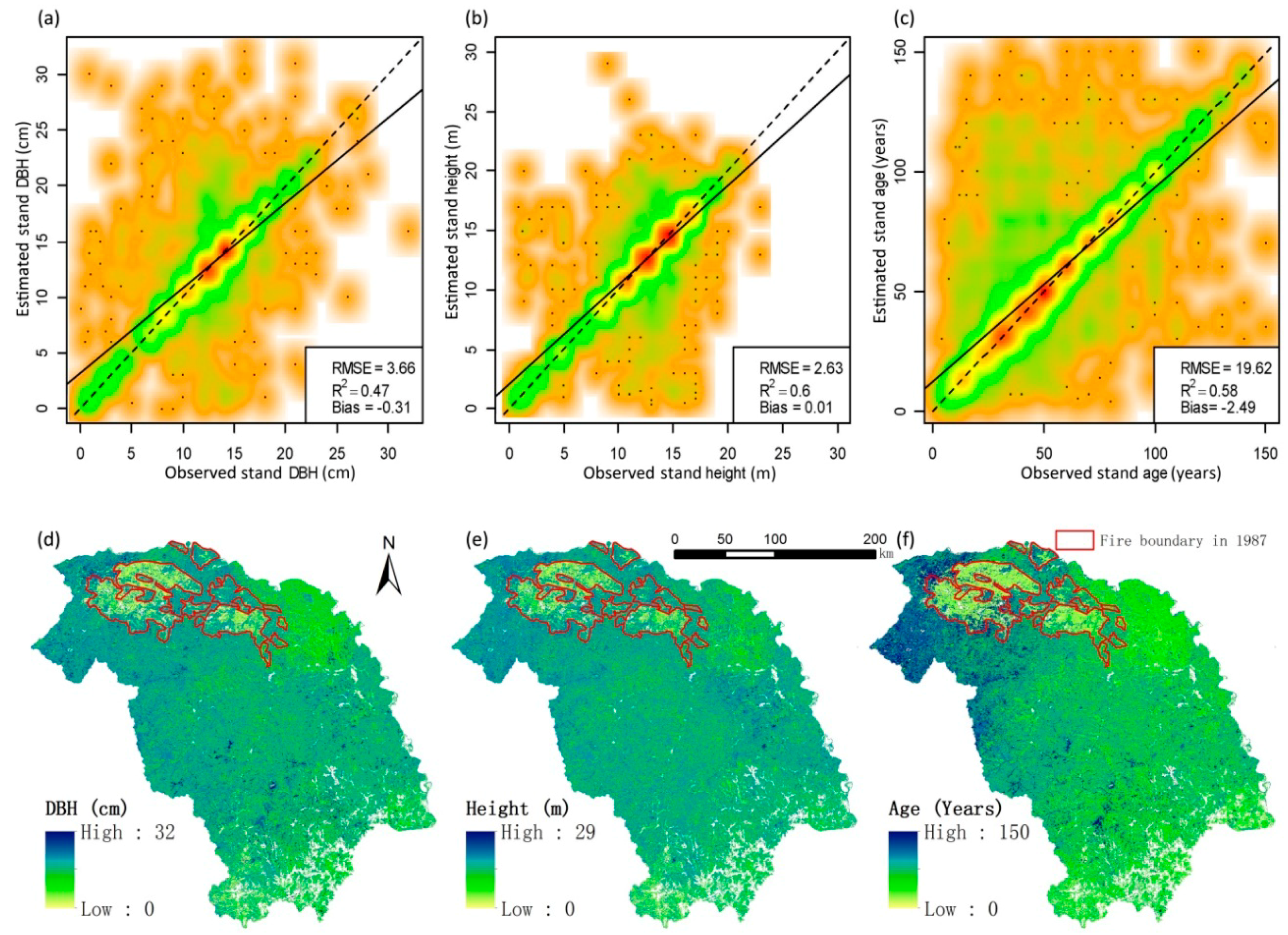
The maps of forest stand DBH, height, and age were estimated at a 250 m spatial resolution using RF-kNN method and assessed using inventory stand polygon data (Figure 3). Results showed that mean estimated values of stand DBH and height were close to their mean observed values with lowest biases (Figure 3a,b), while mean estimated stand age was slightly greater than the observed (Figure 3c). R2 values for the three stand attributes ranged from 0.47 to 0.60, with the highest values for stand height, and the lowest values for stand DBH. RMSE values of the three stand attributes (Figure 3) were relatively accepted compared to their mean observed values (mean stand DBH: 12.55 cm, mean stand height: 12.22 m, mean stand age: 54.56 years).
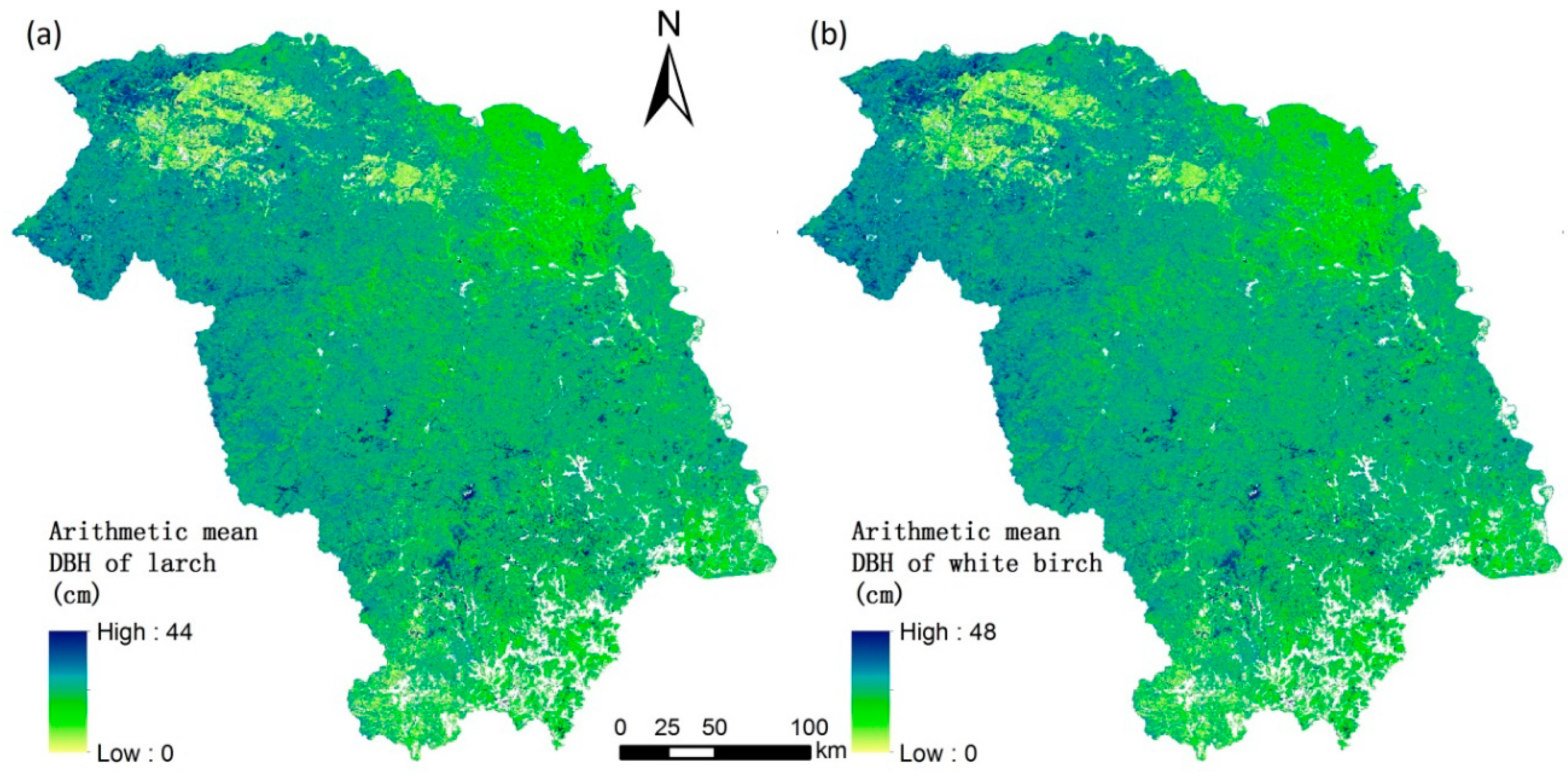
The spatial distributions of three estimated stand attributes were in relation to the area of fire in 1987 and elevations (Figure 3d–f and Figure 1). Fire areas and low elevation areas had consistently low predictions of the three stand attributes. In order to obtain the diameter distributions of larch and white birch in each pixel, arithmetic mean DBH of larch and white birch were also mapped using Equations (4) and (5) based on the three estimated attributes (Figure 4). Because other species often occupied very little proportions of the species composition, we used the mean stand DBH instead of the arithmetic mean DBH of species to calculate their diameter distributions based on the WPPMs in each pixel.

3.3. Maps of Tree Density from Tree-Lists

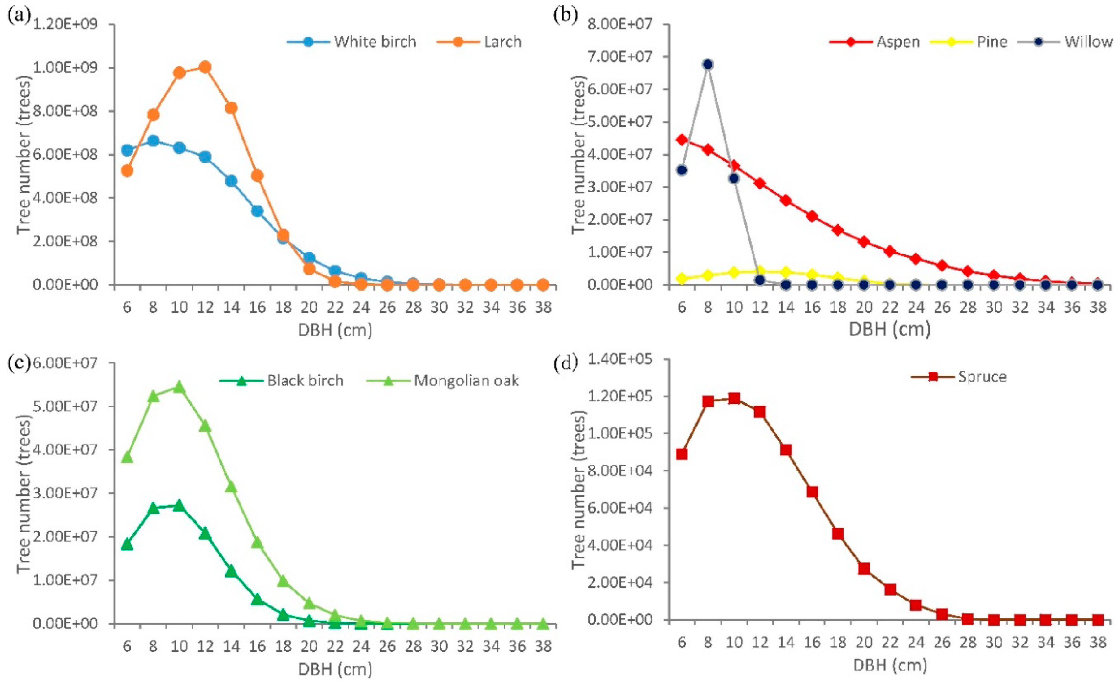
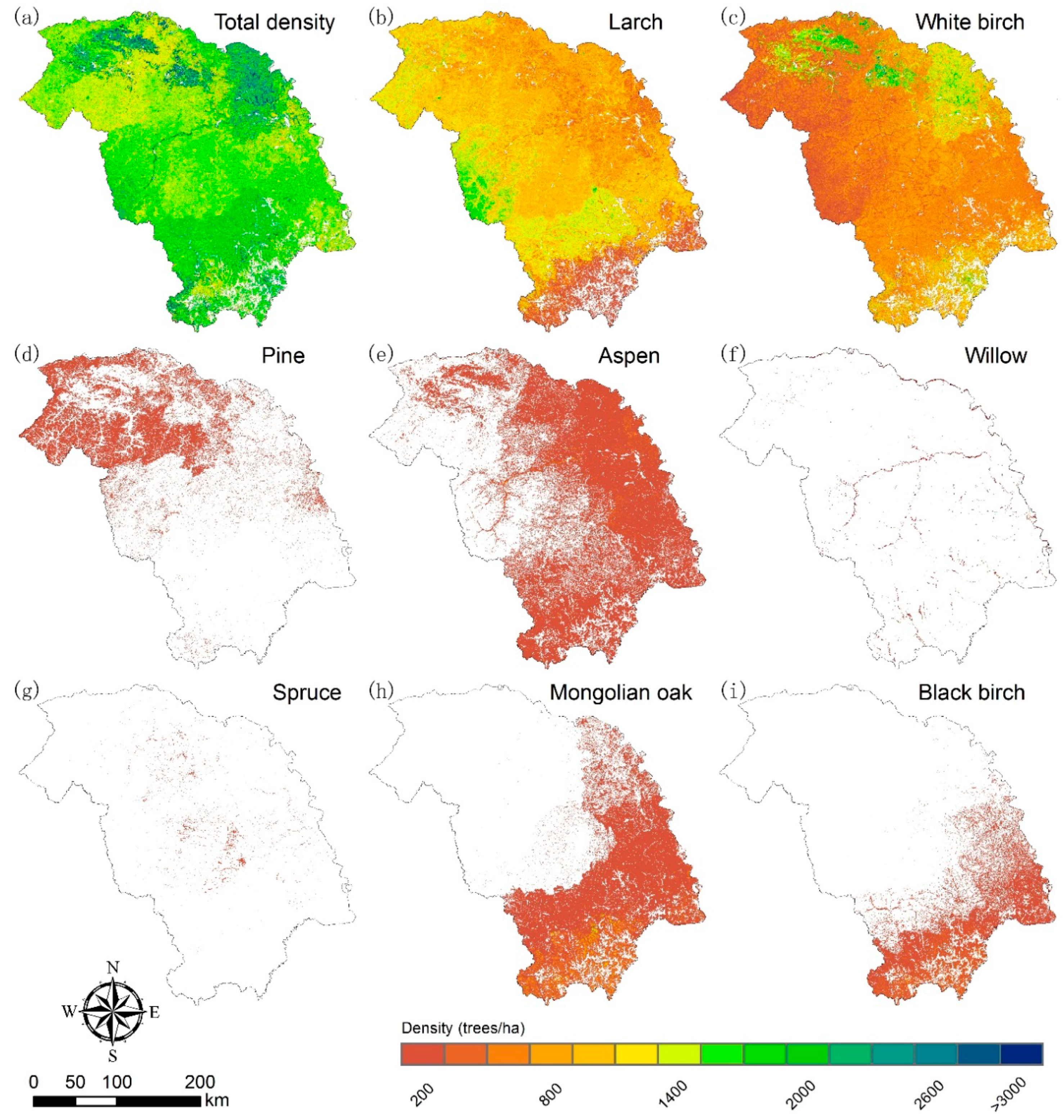
Tree density (trees with DBH >5 cm) of three main forest types derived from estimated tree-lists in 2000s based on WPPMs did not show noticeable difference compared to the observed tree density of the same forest types with a similar environment (Figure 5). The estimated wall-to-wall tree-lists only showed slightly poorer accuracy compared to the estimated tree-lists using stand attributes of plot inventory data in 2011 (Table 4, Figure 6 and Figure 7). When combining all the plots into one data set, the accuracy of tree-lists for most species improved greatly, except for Mongolian oak, and the smallest stems of all species were underestimated (Figure 7). The estimated DBH of most tree species was concentrated in the range of 6 to 22 cm, except for aspen (Figure 8). The total tree density mainly ranged from 500 to 2500 trees/ha (Figure 9). The larch forests with high tree density mainly distributed in places with high elevation. White birch often showed an opposite trend to larch for the spatial tree density distribution, especially in the burned areas in 1987 (Figure 9). For other species, estimated tree density showed less than 450 trees/ha.

4. Discussion

With continuous need of detailed forest attributes (e.g., tree-lists) for answering regional questions, developing methods to obtain such detailed forest attributes attracts a great deal of research interest. Although both the kNN method and Weibull diameter distribution have been widely used for estimating tree-lists [5,9,12,13], the integration of these two methods is novel in generating tree-lists that have seen wide applications. A key novelty of this research is the generation of wall-to-wall estimates of tree-lists over large areas using a limited number of forest ground inventory data.
For reginal forest attribute estimation like this, one important issue is accuracy. Because wall-to-wall tree-lists estimated by our framework are transformed from species-level biomass by kNN imputation and tree density percent from WPPMs, the accuracy of our estimated tree-lists were mainly determined by WPPMs and kNN imputation models. For a more general assessment of our method framework, we compared the accuracies of WPPMs and kNN models with other similar studies. We found that the parameter prediction models of Weibull diameter distributions (WPPMs) in our study produced comparable accuracy with the previous studies. For example, Liu [40] reported that the determination coefficient (R2) of the shape parameter (b) estimated by the previous parameter prediction models (PPMs) was generally close to 0.1—slightly poorer than our results. Additionally, our estimates of scale parameter (c) for all the species were slightly better than the results that Diamantopoulou et al., reported in the south and southwestern (Mediterranean) regions of Turkey (c: R2 = 0.96–0.99). The mean error index (0.32–0.34) of the estimated diameter distributions in a typical Finnish managed boreal forest area that Packalén and Maltamo reported was similar to our results about the dominant tree species. These comparisons indicate that our WPPMs can be used at least as accurately as previous studies to estimate tree diameter distribution.
Our imputed wall-to-wall stand attributes (e.g., stand DBH, height, and age) also showed comparable accuracy to the previous similar studies. For example, the accuracy of our study was very close to the results that Beaudoin et al. (2014) [41] reported about the stand age and height in a Canadian forest, with R2 of 0.57 and 0.58, RMSE 44.29 years and 5.66 m, and bias of 1.54 years and 0.07 m. In addition, the area with low estimated values of stand DBH, height, and age was consistent with the area disturbed by fires in 1987 and low elevations linked to intensive human activities, indicating that our spatial predictions of forest attributes are realistic, capturing dominant ecological patterns and processes.
Although we were unable to directly assess the accuracy of the estimated tree-lists in the 2000s due to the lack of tree-lists inventory data in this period, the assessments of WPPMs and kNN imputation models in our study demonstrated that our estimated tree-lists had comparable accuracy to previous studies. The assessment of the estimated tree-lists in 2000 based on transformed inventory tree-lists data provided the accuracy about our method framework, which were comparable with a previous study that was in much smaller area [12]. The comparisons between estimated and observed total density also indicated that the estimated tree-lists in 2000s had no obvious difference with tree-lists from the forest inventory in 2011 with the same forest types and similar environmental conditions. In addition, the estimated tree density ranging from 400 to 2500 trees/ha (Figure 9) (DBH ≥ 5 cm) is consistent with the previous results reported by Zhai, et al. [42] and Zhao et al. [43]. These comparisons also indicated that the estimated tree-lists had a relatively reliable accuracy.
There are many methods to describe the diameter distributions of forests stands, among which the Weibull function is one of the most simple and accurate functions for modeling diameter distribution. Liu et al. [44] compared three methods of Weibull function in modeling diameter distributions in Daxing’an Mountain, China. They found that a finite mixture model (FMM) of Weibull functions was more flexible to describe highly skewed and irregular diameter distributions than a single Weibull function to fit the whole stand only, and a single Weibull function to fit each species component separately was also able to fit each species component well in mixed forest stands. However, FMM is often difficult to use for large regions due to many unknown parameters requiring estimation [45]. A single Weibull function to fit each species component separately is easy to use but first requires the information of species composition, which is also difficult to obtain only through the forest inventory across large regions. Our method framework could use a Weibull function to fit each species component separately and provide the information about species composition across large regions using a kNN model based on MODIS data. MODIS data have wide coverage and high temporal resolution, and have been widely used to generate regional maps of forest attributes [3,5,24,30,41,46,47,48,49,50]. The advantage of our method framework is its use of MODIS data as predictor variables to estimate stand attributes. Compared to other high-resolution optical images (e.g., Landsat), MODIS data provide abundant and near-real-time information for the forest stand attribute imputation across large regions [14,30]. Therefore, our framework may be more feasible for use across large regions to describe diameter distributions.
Many approaches have been used to estimate Weibull parameters for describing diameter distributions such as ordinary least squares (OLS), seemingly unrelated regression (SUR), cumulative distribution function regression (CDFR), or artificial neural network (ANN) methods [21]. Although Diamantopoulou et al. [20] proved that complex methods (e.g., ANN) were superior to simple methods (e.g., OLS) in the estimation of Weibull parameters, the application of complex methods is often limited across large regions because they are often based on a training method and their results cannot go not beyond the range of training samples. The OLS method is simple and has been widely used to fit the parameter models. Additionally, many previous studies have also proved that it was possible to estimate the scale or shape parameters of a two-parameter Weibull function using the parametric models fitted by OLS [51,52]. Therefore, in this study parametric WPPMs were built using only OLS.
In this study, only the arithmetic DBHs of larch and white birch were calculated and used when estimating the wall-to-wall species’ diameter distribution. For other species, we used stand DBH instead of tree species’ arithmetic DBH to estimate the parameters of Weibull diameter distribution because of their small percentage of forest species composition for most forest stands in our study area. Although it is reasonable for the Chinese boreal forests, which have simple stand structures, great uncertainties might be produced for forests with complicated structures using stand DBH instead of tree species’ arithmetic DBH. Therefore, our method framework is generally suited for forests with simple stand structure, such as boreal forests.

5. Conclusions

Wall-to-wall tree-lists across large regions are required to support science, policy, and reporting information requirements. However, it is difficult to obtain such information across large regions due to the high cost of the forest inventory. In this study, we presented a framework to estimate wall-to-wall tree-lists using limited forest inventory plots by integrating a Weibull diameter distribution with the imputed stand attributes based on the kNN method in Chinese boreal forests. The Weibull function showed strong ability to describe the diameter distributions of tree species. The WPPMs of six species showed acceptable accuracy for estimating the parameters of Weibull functions. The imputed stand age, mean height, and DBH across the study area by the kNN method also showed comparable accuracy with previous study. The estimated tree density derived from tree-lists did not show obvious difference between the observed and estimated data for similar forest types. Our estimated tree-lists also captured some effects of ecological processes, such as fire disturbance. Our method provides an alternative for estimating the tree lists over large area such as the boreal forest biome in China.

Author Contributions

The authors provided equal contribution towards decisions regarding methodology and study design. Early drafts were written by Q.Z., and revised and edited by Y.L., and H.S.H.

Funding

This research was funded by National Key Research and Development Program of China (grant numbers: 2017YFA0604402 and 2016YFA0600804), and National Natural Science Foundation of China (grant number: 31570461).

Acknowledgments

Thanks to the anonymous reviewers for their constructive and valuable comments, and the editors for their assistance in refining this article.

Conflicts of Interest

The authors declare no conflict of interest. The funding sponsors had no role in the design of the study; in the collection, analyses, or interpretation of data; in the writing of the manuscript; or in the decision to publish the results.

References

  1. Temesgen, B.H.; LeMay, V.M.; Froese, K.L.; Marshall, P.L. Imputing tree-lists from aerial attributes for complex stands of south-eastern British Columbia. For. Ecol. Manag. 2003, 177, 277–285. [Google Scholar] [CrossRef]
  2. Xiao, J.; Liang, Y.; He, H.S.; Thompson, J.R.; Wang, W.J.; Fraser, J.S.; Wu, Z. The formulations of site-scale processes affect landscape-scale forest change predictions: A comparison between LANDIS PRO and LANDIS-II forest landscape models. Landsc. Ecol. 2017, 32, 1347–1363. [Google Scholar] [CrossRef]
  3. Duveneck, M.J.; Thompson, J.R.; Wilson, B.T. An imputed forest composition map for New England screened by species range boundaries. For. Ecol. Manag. 2015, 347, 107–115. [Google Scholar] [CrossRef]
  4. Liang, Y.; Duveneck, M.J.; Gustafson, E.J.; Serradiaz, J.M.; Thompson, J.R. How disturbance, competition, and dispersal interact to prevent tree range boundaries from keeping pace with climate change. Glob. Chang. Biol. 2018, 24, e335–e351. [Google Scholar] [CrossRef] [PubMed]
  5. Zald, H.S.J.; Ohmann, J.L.; Roberts, H.M.; Gregory, M.J.; Henderson, E.B.; McGaughey, R.J.; Braaten, J. Influence of lidar, Landsat imagery, disturbance history, plot location accuracy, and plot size on accuracy of imputation maps of forest composition and structure. Remote Sens. Environ. 2014, 143, 26–38. [Google Scholar] [CrossRef]
  6. Crowther, T.W.; Glick, H.B.; Covey, K.R.; Bettigole, C.; Maynard, D.S.; Thomas, S.M.; Smith, J.R.; Hintler, G.; Duguid, M.C.; Amatulli, G.; et al. Mapping tree density at a global scale. Nature 2015, 525, 201–205. [Google Scholar] [CrossRef] [PubMed]
  7. Eerikäinen, K.; Maltamo, M. A percentile based basal area diameter distribution model for predicting the stand development of Pinus kesiya plantations in Zambia and Zimbabwe. For. Ecol. Manag. 2003, 172, 109–124. [Google Scholar] [CrossRef]
  8. Ohmann, J.L.; Gregory, M.J. Predictive mapping of forest composition and structure with direct gradient analysis and nearest-neighbor imputation in coastal Oregon, USA. Can. J. For. Res.-Rev. Can. De Rech. For. 2002, 32, 725–741. [Google Scholar] [CrossRef]
  9. Lamb, S.M.; MacLean, D.A.; Hennigar, C.R.; Pitt, D.G. Imputing tree lists for New Brunswick spruce plantations through nearest-neighbor matching of airborne laser scan and inventory plot data. Can. J. Remote Sens. 2017, 43, 269–285. [Google Scholar] [CrossRef]
  10. Maltamo, M.; Gobakken, T. Predicting tree diameter distributions. In Forestry Applications of Airborne Laser Scanning: Concepts and Case Studies; Maltamo, M., Næsset, E., Vauhkonen, J., Eds.; Springer: Dordrecht, The Netherlands, 2014; pp. 177–191. [Google Scholar]
  11. Lindberg, E.; Holmgren, J.; Olofsson, K.; Wallerman, J.R.; Olsson, H.K. Estimation of Tree Lists from Airborne Laser Scanning Using Tree Model Clustering and k-MSN Imputation. Remote Sens. 2013, 5, 1932–1955. [Google Scholar] [CrossRef] [Green Version]
  12. Packalén, P.; Maltamo, M. Estimation of species-specific diameter distributions using airborne laser scanning and aerial photographs. Can. J. For. Res. 2008, 38, 1750–1760. [Google Scholar] [CrossRef]
  13. Bollandsås, O.M.; Maltamo, M.; Gobakken, T.; Næsset, E. Comparing parametric and non-parametric modelling of diameter distributions on independent data using airborne laser scanning in a boreal conifer forest. Forestry 2013, 86, 493–501. [Google Scholar] [CrossRef]
  14. Wilson, B.T.; Lister, A.J.; Riemann, R.I. A nearest-neighbor imputation approach to mapping tree species over large areas using forest inventory plots and moderate resolution raster data. For. Ecol. Manag. 2012, 271, 182–198. [Google Scholar] [CrossRef]
  15. Moeur, M.; Stage, A.R. Most similar neighbor: An improved sampling inference procedure for natural resource planning. For. Sci. 1995, 41, 337–359. [Google Scholar] [CrossRef]
  16. Breiman, L. Random forests. Mach. Learn. 2001, 45, 5–32. [Google Scholar] [CrossRef]
  17. Nanos, N.; Montero, G. Spatial prediction of diameter distribution models. For. Ecol. Manag. 2002, 161, 147–158. [Google Scholar] [CrossRef]
  18. Van Deusen, P.C. Annual forest inventory statistical concepts with emphasis on multiple imputation. Can. J. For. Res. 1997, 27, 379–384. [Google Scholar] [CrossRef]
  19. McRoberts, R.E. Diagnostic tools for nearest neighbors techniques when used with satellite imagery. Remote Sens. Environ. 2009, 113, 489–499. [Google Scholar] [CrossRef]
  20. Diamantopoulou, M.J.; Özçelik, R.; Crecente-Campo, F.; Eler, Ü. Estimation of Weibull function parameters for modelling tree diameter distribution using least squares and artificial neural networks methods. Biosyst. Eng. 2015, 133, 33–45. [Google Scholar] [CrossRef]
  21. Poudel, K.P.; Cao, Q.V. Evaluation of methods to predict Weibull parameters for characterizing diameter distributions. For. Sci. 2013, 59, 243–252. [Google Scholar] [CrossRef]
  22. Matasci, G.; Hermosilla, T.; Wulder, M.A.; White, J.C.; Coops, N.C.; Hobart, G.W.; Zald, H.S.J. Large-area mapping of Canadian boreal forest cover, height, biomass and other structural attributes using Landsat composites and lidar plots. Remote Sens. Environ. 2018, 209, 90–106. [Google Scholar] [CrossRef]
  23. Zald, H.S.J.; Wulder, M.A.; White, J.C.; Hilker, T.; Hermosilla, T.; Hobart, G.W.; Coops, N.C. Integrating Landsat pixel composites and change metrics with lidar plots to predictively map forest structure and aboveground biomass in Saskatchewan, Canada. Remote Sens. Environ. 2016, 176, 188–201. [Google Scholar] [CrossRef]
  24. Li, L.; Guo, Q.; Tao, S.; Kelly, M.; Xu, G. Lidar with multi-temporal MODIS provide a means to upscale predictions of forest biomass. ISPRS J. Photogramm. Remote Sens. 2015, 102, 198–208. [Google Scholar] [CrossRef]
  25. Podlaski, R.; Roesch, F.A. Modelling diameter distributions of two-cohort forest stands with various proportions of dominant species: A two-component mixture model approach. Math. Biosci. 2014, 249, 60–74. [Google Scholar] [CrossRef]
  26. Zhou, Y. Vegetation of Da Hinggan Ling in China; China Science Press: Beijing, China, 1991. [Google Scholar]
  27. Xu, H. Forest in Great Xing’an Mountains of China; China Science Press: Beijing, China, 1998. [Google Scholar]
  28. Liu, Z.; He, H.S.; Yang, J.; Collins, B. Emulating natural fire effects using harvesting in an eastern boreal forest landscape of northeast China. J. Veg. Sci. 2012, 23, 782–795. [Google Scholar] [CrossRef]
  29. Zhang, Y.; Liang, S. Changes in forest biomass and linkage to climate and forest disturbances over Northeastern China. Glob. Chang. Biol. 2014, 20, 2596–2606. [Google Scholar] [CrossRef] [PubMed]
  30. Zhang, Q.; He, H.S.; Liang, Y.; Hawbaker, T.J.; Henne, P.D.; Liu, J.; Huang, S.; Wu, Z.; Huang, C. Integrating forest inventory data and MODIS data to map species-level biomass in Chinese boreal forests. Can. J. For. Res. 2018, 48, 461–479. [Google Scholar] [CrossRef]
  31. Mao, D.; Wang, Z.; Luo, L.; Ren, C. Integrating AVHRR and MODIS data to monitor NDVI changes and their relationships with climatic parameters in Northeast China. Int. J. Appl. Earth Obs. Geoinf. 2012, 18, 528–536. [Google Scholar] [CrossRef]
  32. Venables, W.N.; Ripley, B.D. Modern Applied Statistics with S. Fourth Edition; Springer: New York, NY, USA, 2002. [Google Scholar]
  33. Coreteam, R. R: A Language and Environment for Statistical Computing; R Foundation for Statistical Computing: Vienna, Austria, 2015. [Google Scholar]
  34. Qi, Y. Estimates of Forest Above Ground Carbon Storage Using Remote Sensing in Daxing’an Mountains. Ph.D. Thesis, Northeast Forestry University, Haerbin, China, June 2014. [Google Scholar]
  35. Feng, Z. The Biomass and Productivity of Forest Ecosystem in China; China Science Press: Beijing, China, 1999. [Google Scholar]
  36. Lopes, R.H.C.; Reid, I.; Hobson, P.R. The two-dimensional Kolmogorov-Smirnov test. In Proceedings of the XI International Workshop on Advanced Computing & Analysis Techniques in Physics Research, Amsterdam, The Netherlands, 23–27 April 2007; pp. 196–206. [Google Scholar]
  37. Riemann, R.; Wilson, B.T.; Lister, A.; Parks, S. An effective assessment protocol for continuous geospatial datasets of forest characteristics using USFS Forest Inventory and Analysis (FIA) data. Remote Sens. Environ. 2010, 114, 2337–2352. [Google Scholar] [CrossRef]
  38. Kankare, V.; Liang, X.; Vastaranta, M.; Yu, X.; Holopainen, M.; Hyyppä, J. Diameter distribution estimation with laser scanning based multisource single tree inventory. ISPRS J. Photogramm. Remote Sens. 2015, 108, 161–171. [Google Scholar] [CrossRef]
  39. Zhou, Z. Study on Biomass and Carbon Storage of Main Fuel Type in DaXing'AnLing Mountain. Ph.D. Thesis, Northeast Forestry University, Haerbin, China, June 2006. [Google Scholar]
  40. Liu, F. Diameter Distributions of Individual Species Components of Natural Mixed Forest of Larix Gmelini—Betula Platyphylla in Dazing’an Mountains. Ph.D. Thesis, Northeast Forestry University, Haerbin, China, June 2013. [Google Scholar]
  41. Beaudoin, A.; Bernier, P.Y.; Guindon, L.; Villemaire, P.; Guo, X.J.; Stinson, G.; Bergeron, T.; Magnussen, S.; Hall, R.J. Mapping attributes of Canada’s forests at moderate resolution through kNN and MODIS imagery. Can. J. For. Res. 2014, 44, 521–532. [Google Scholar] [CrossRef]
  42. Zhai, M.; Yin, W.; Jia, L.; Ma, L.; Sun, Y.; Liu, Z.; Wang, Y. Investigation and study on mixed forest of Hingan larch and white birch in Xilinji. J. Northeast. For. Univ. 1990, 12, 78–85. [Google Scholar] [CrossRef]
  43. Zhao, H.; Wang, Y.; Li, J.; He, X. The age structure, horizontal pattern and management of natural deciduous larch forest in Tahe Forestry Bureau. J. Northeast For. Univ. 1987, 15, 80–85. [Google Scholar] [CrossRef]
  44. Liu, F.; Li, F.; Zhang, L.; Jin, X. Modeling diameter distributions of mixed-species forest stands. Scand. J. For. Res. 2014, 29, 653–663. [Google Scholar] [CrossRef]
  45. Zasada, M.; Cieszewski, C.J. A finite mixture distribution approach for characterizing tree diameter distributions by natural social class in pure even-aged Scots pine stands in Poland. For. Ecol. Manag. 2005, 204, 145–158. [Google Scholar] [CrossRef]
  46. Beaudoin, A.; Bernier, P.Y.; Villemaire, P.; Guindon, L.; Guo, X.J. Tracking forest attributes across Canada between 2001 and 2011 using a k nearest neighbors mapping approach applied to MODIS imagery. Can. J. For. Res. 2018, 48, 85–93. [Google Scholar] [CrossRef]
  47. Pouliot, D.; Latifovic, R.; Zabcic, N.; Guindon, L.; Olthof, I. Development and assessment of a 250m spatial resolution MODIS annual land cover time series (2000–2011) for the forest region of Canada derived from change-based updating. Remote Sens. Environ. 2014, 140, 731–743. [Google Scholar] [CrossRef]
  48. Wang, Y.; Li, G.; Ding, J.; Guo, Z.; Tang, S.; Wang, C.; Huang, Q.; Liu, R.; Chen, J.M. A combined GLAS and MODIS estimation of the global distribution of mean forest canopy height. Remote Sens. Environ. 2016, 174, 24–43. [Google Scholar] [CrossRef] [Green Version]
  49. Ferreira, M.P.; Zortea, M.; Zanotta, D.C.; Shimabukuro, Y.E.; de Souza Filho, C.R. Mapping tree species in tropical seasonal semi-deciduous forests with hyperspectral and multispectral data. Remote Sens. Environ. 2016, 179, 66–78. [Google Scholar] [CrossRef]
  50. Zhu, X.; Liu, D. Improving forest aboveground biomass estimation using seasonal Landsat NDVI time-series. ISPRS J. Photogramm. Remote Sens. 2015, 102, 222–231. [Google Scholar] [CrossRef]
  51. Meng, X. A study of the relation between d and h distribution by using the weibull function. J. Beijing For. Univ. 1988, 10, 40–48. [Google Scholar] [CrossRef]
  52. Fang, J.; Jian, C. Estimating diameter distribution with the weibull distribution function. J. Beijing For. Univ. 1987, 9, 261–269. [Google Scholar] [CrossRef]
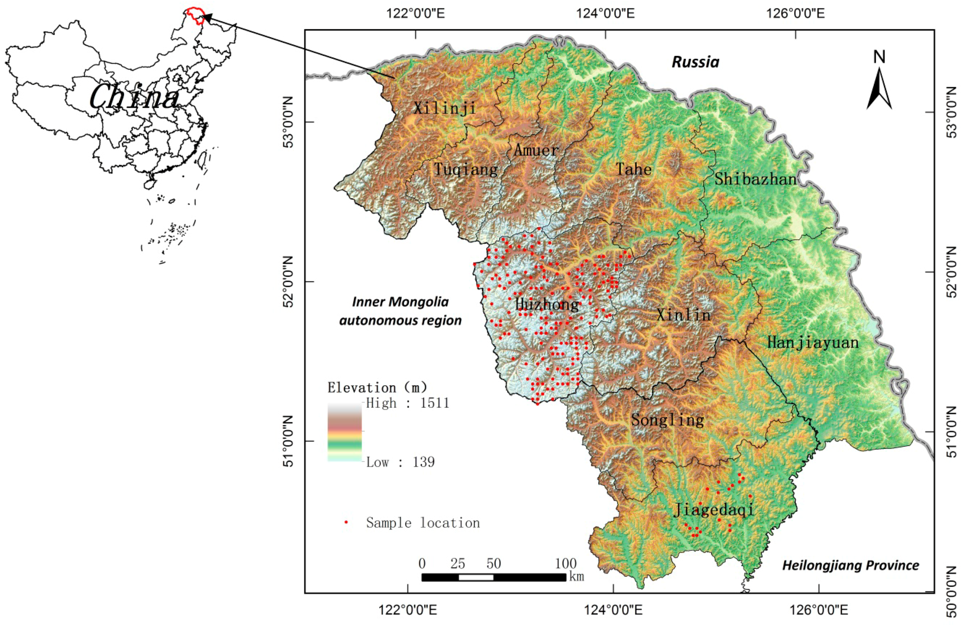
Figure 1. The location and elevation of the study area with the distribution of the forest inventory plots (red plots).
Forests 09 00758 g001
Figure 2. The overall framework of generating tree-lists. DBH: Diameter at breast height; kNN, k-nearest neighbor; WPPMs, Weibull parameter prediction models by species.
Forests 09 00758 g002
Figure 3. Goodness-of-fittings (density scatterplots) of the random forest (RF)-based kNN models of stand DBH, height, and age (ac) and maps of estimated diameter, height, and age (df). The points superimposed on the density image are the points from those areas of lowest regional densities, which are the identification of outliers. The dotted line is the 1:1 line and the dashed line is the geometric mean functional regression line.
Forests 09 00758 g003
Figure 4. Maps of arithmetic mean DBH of larch (a) and white birch (b) based on Equations (4) and (5).
Forests 09 00758 g004
Figure 5. Boxplots of observed vs. predicted tree density of three main forest types (Larch forests (a), White birch forests (b) and Mixed forests (c)) with similar environment (p > 0.05). Observed tree density was calculated from the inventory plot data in 2011. Estimated tree density was calculated from the estimated tree-lists in 2000s. The same letter “a” indicated that there was no obvious difference between observed and estimated tree density.
Forests 09 00758 g005
Figure 6. Error indices of estimated wall-to-wall tree-lists by species in 2000 based on the transformed inventory tree-lists data. The error indices were calculated by each transformed plot.
Forests 09 00758 g006
Figure 7. DBH distributions by species (larch (a), white birch (b), pine (c), aspen (d), spruce (e), Mongolian oak (f)) of the observed vs. estimated wall-to-wall tree-lists based on the transformed inventory tree-lists data. The error indices were calculated by regarding all transformed plots as a whole.
Forests 09 00758 g007
Figure 8. Estimated tree-lists of the study area in 2000 by species (larch and white birch (a); aspen, pine and willow (b); black birch and Mongolian oak (c); spruce (d)).
Forests 09 00758 g008
Figure 9. Maps of estimated total stand density and stand density by species (total density (a), larch (b), white birch (c), pine (d), aspen (e), willow (f), spruce (g), Mongolian oak (h) and black birch (i)).
Forests 09 00758 g009
Table 1. Equations of DBH (d, unit: cm) and age (a, unit: year) for six species and accuracy assessment using leave-one-out cross validation (LOOCV). RMSE: Root mean square error.
SpeciesEquationsR2RMSEBiasp-value
Larchd = 0.1972a + 1.57010.961.950.040.00
White birchd = 0.2287a + 2.2220.960.950.000.00
Pined = 0.2659a − 1.470.754.880.000.00
Aspend = 0.3405a − 0.270.922.860.000.00
Spruced = 0.1154a + 7.69190.333.160.000.00
Mongolian oakd = 0.1333a + 3.26790.871.890.000.00
Table 2. The agreement of each species for the two-parameter Weibull diameter distribution using Kolmogorov–Smirnov (KS) test (p > 0.05).
SpeciesSamples Passing the KS TestSample NumberAgreement (%)
Larch13415288.16
White birch637584.00
Pine354185.36
Aspen264065.00
Spruce273577.14
Mongolian oak122157.14
Willow11100.00
* Agreement is the percentage of the samples that the passed the KS test.
Table 3. Equations of shape parameter (b) and scale parameter (c) of Weibull diameter distribution depend on arithmetic mean DBH (d, unit: cm) for each species and accuracy assessment using leave-one-out cross validation (LOOCV).
SpeciesEquationsR2RMSEBiasp-value
Larchb = 0.16782d + 1.622850.171.870.000.00
c = 1.067865d − 0.5088241.000.340.000.00
White birchb = −0.18218d + 5.078480.220.740.000.00
c = 1.153572d − 0.3471481.000.120.000.00
Pineb = 0.22833d + 0.089270.201.110.000.01
c = 1.08108d + 0.513440.990.210.000.00
Aspenb = −1.16886d + 4.959780.310.580.000.00
c = 1.153572d − 0.3591691.000.080.000.00
Spruceb = −0.21014d + 4.703190.290.470.000.00
c = 1.16454d − 0.3573221.000.070.000
Mongolian oakb = 0.068193d + 1.2454810.131.140.000.06
c = 1.140851d − 0.212071.000.560.000
Table 4. Error indices of DBH distributions for each species in all plots based on the WPPMs using LOOCV method.
SpeciesMean Value of Error IndicesMinimum Value of Error IndicesMaximum Value of Error IndicesStandard Deviation of Error IndicesError Indices of Summing All the Plots
Larch0.330.100.890.150.11
White birch0.270.090.800.130.08
Pine0.390.170.870.180.06
Aspen0.430.170.790.190.04
Spruce0.400.170.740.160.14
Mongolian oak0.620.510.800.090.06
* Error indices of summing all the plots are the error indices calculated by regarding all plots as a whole.