Evaluating Two Optical Methods of Woody-to-Total Area Ratio with Destructive Measurements at Five Larix gmelinii Rupr. Forest Plots in China

Abstract
1. Introduction
2. Theory
2.1. Effective PAI (), Effective WAI (), PAI, and WAI
2.2. Effective Woody-to-Total Area Ratio () and Woody-to-Total Area Ratio ()
3. Materials and Methods
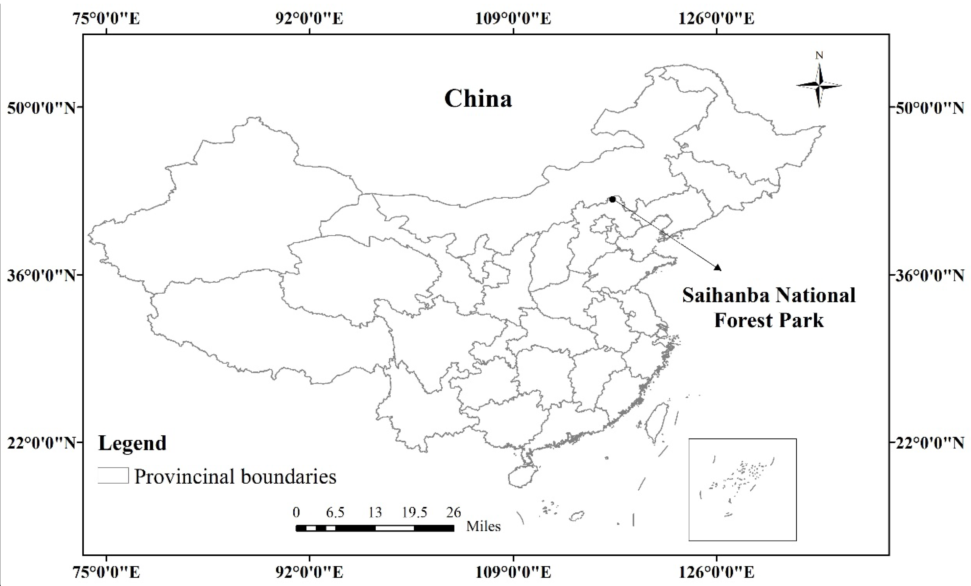
3.1. Plots Description
3.2. Mean Element Eidth and Needle-to-Shoot Area Ratio () Measurement
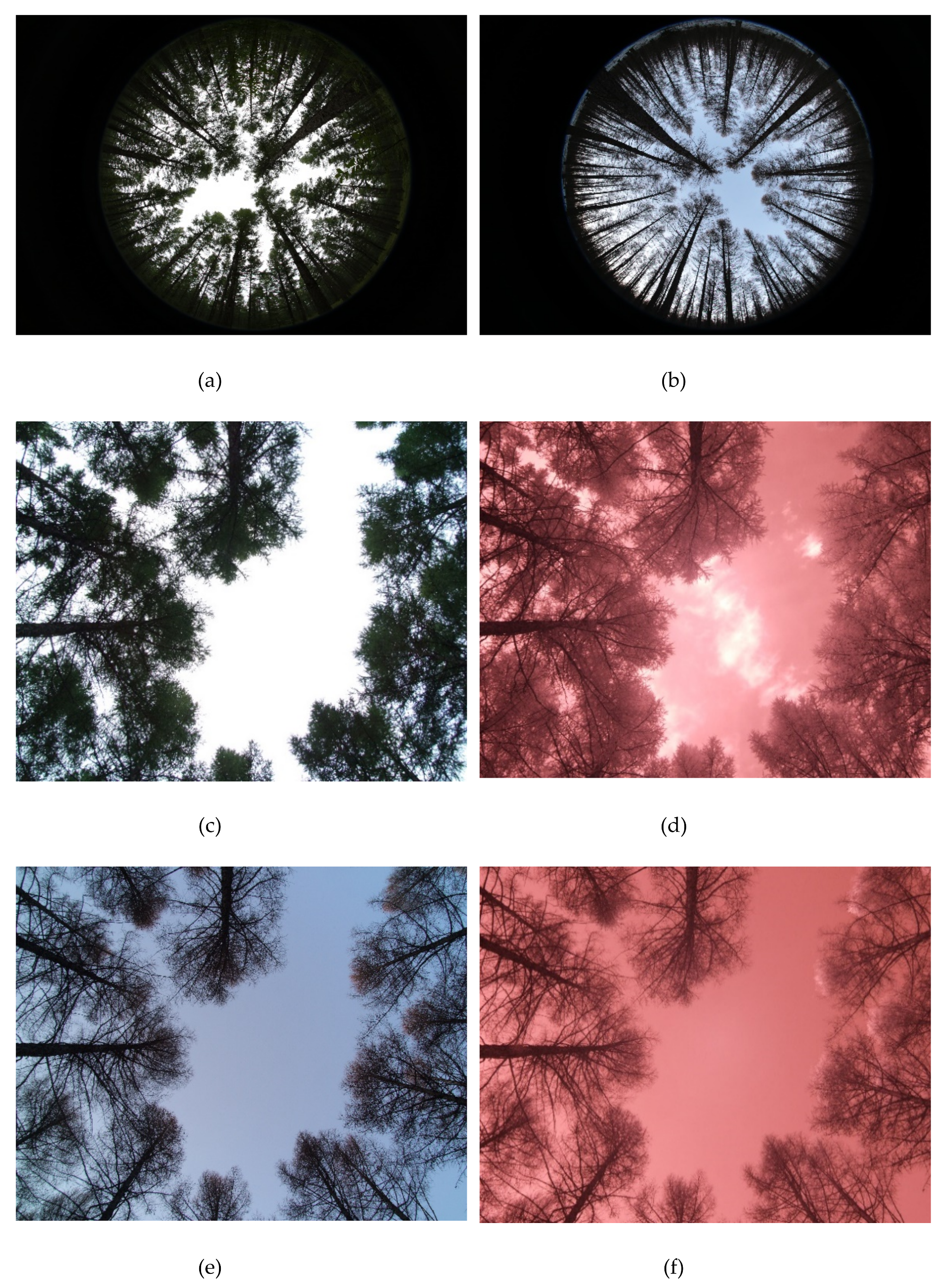
3.3. DHP Images Acquisition and Processing
3.4. MCI Images Acquisition and Processing
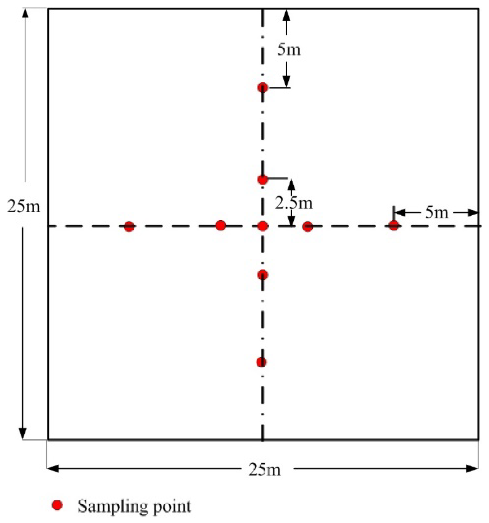
3.5. The Measurements of The Representative Trees and Plots
4. Results
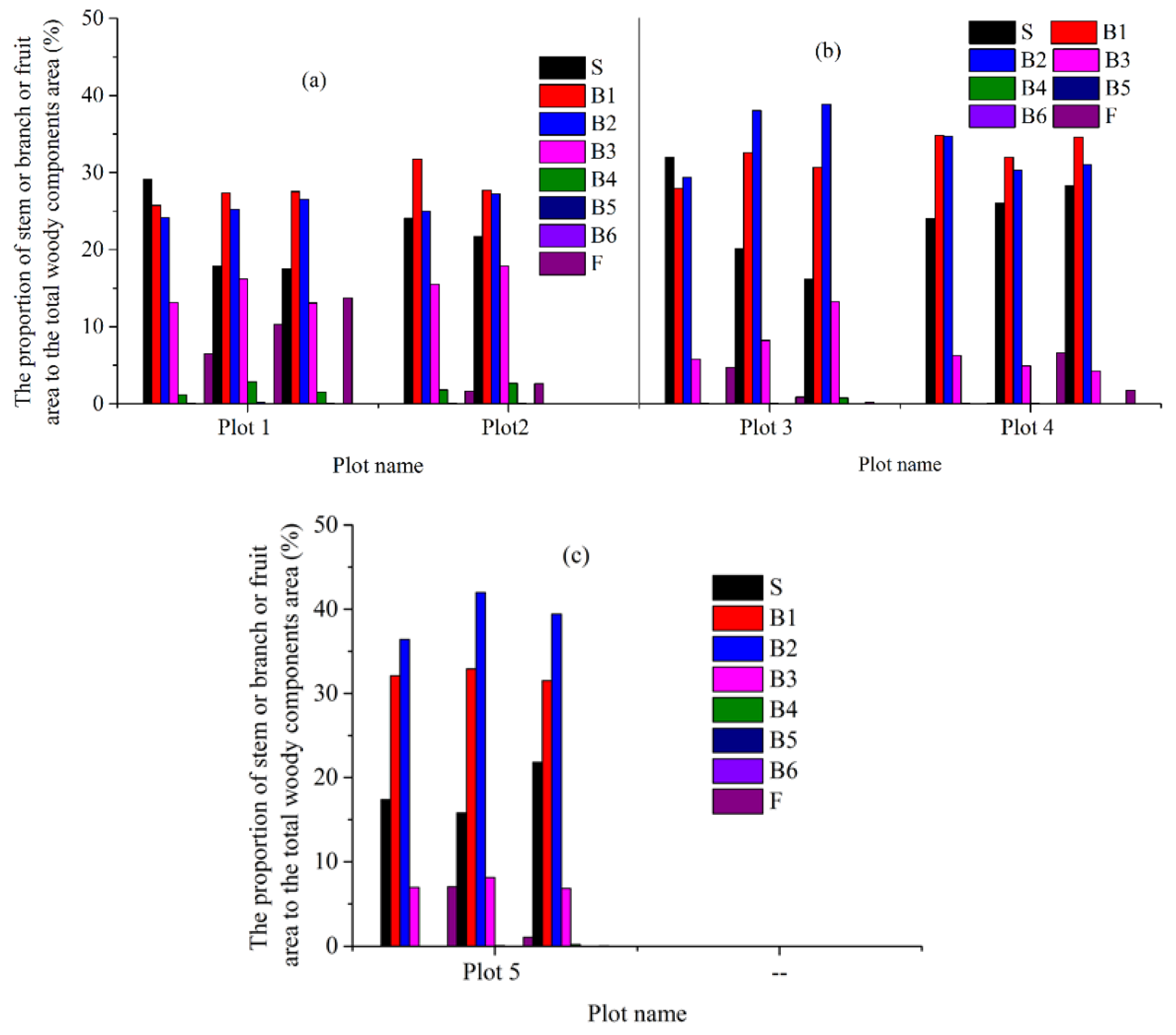
4.1. Estimates Obtained from The Destructive Method
4.2. Estimates Obtained from DHP and MCI
4.3. Estimates Obtained from DHP and MCI
5. Discussion
5.1. Factors That Affect the Accuracy of the Reference Estimates
5.2. Impact of Tree Age, Stand Density, Site Conditions, and Management Activities on the Reference of Forest Plots
5.3. Factors That Affect the Estimation of the Two Optical Methods
5.4. Determining Whether Accurate Estimates Can Be Obtained from DHP and MCI
5.5. Limitations and Perspectives
6. Conclusions
Author Contributions
Funding
Conflicts of Interest
Appendix
References
- Fernandes, R.; Plummer, S.; Nightingale, J.; Baret, F.; Camacho, F.; Fang, H.; Garrigues, S.; Gobron, N.; Lang, M.; Lacaze, R.; et al. Global Leaf Area Index Product Validation Good Practices (Version 2.0). In Best Practice for Satellite-Derived Land Product Validation (p. 76): Land Product Validation Subgroup (WGCV/CEOS); Gabriela, S.-S., Miguel, R., Eds.; NOAA, USGS, NASA, College Park: USA, 2014. [Google Scholar]
- Watson, D.J. Comparative physiological studies in the growth of field crops. I. Variation in net assimilation rate and leaf area between species and varieties, and within and between years. Ann. Bot. 1947, 11, 41–76. [Google Scholar] [CrossRef]
- Chen, J.M.; Black, T.A. Defining leaf area index for non-flat leaves. Plant. Cell. Environ. 1992, 15, 421–429. [Google Scholar] [CrossRef]
- Baret, F.; Hagolle, O.; Geiger, B.; Bicheron, P.; Miras, B.; Huc, M.; Berthelot, B.; Niño, F.; Weiss, M.; Samain, O.; et al. Lai, fapar and fcover cyclopes global products derived from vegetation: Part 1: Principles of the algorithm. Remote Sens. Environ. 2007, 110, 275–286. [Google Scholar] [CrossRef]
- Feng, D.; Chen, J.M.; Plummer, S.; Mingzhen, C.; Pisek, J. Algorithm for global leaf area index retrieval using satellite imagery. IEEE Trans. Geosci. Remote Sens. 2006, 44, 2219–2229. [Google Scholar] [CrossRef]
- Xiao, Z.; Liang, S.; Wang, J.; Chen, P.; Yin, X.; Zhang, L.; Song, J. Use of general regression neural networks for generating the glass leaf area index product from time-series modis surface reflectance. IEEE Trans. Geosci. Remote Sens. 2014, 52, 209–223. [Google Scholar] [CrossRef]
- Knyazikhin, Y.; Martonchik, J.V.; Myneni, R.B.; Diner, D.J.; Running, S.W. Synergistic algorithm for estimating vegetation canopy leaf area index and fraction of absorbed photosynthetically active radiation from modis and misr data. J. Geophys. Res. Atmos. 1998, 103, 32257–32275. [Google Scholar] [CrossRef]
- Baret, F.; Weiss, M.; Lacaze, R.; Camacho, F.; Makhmara, H.; Pacholcyzk, P.; Smets, B. Geov1: Lai and fapar essential climate variables and fcover global time series capitalizing over existing products. Part1: Principles of development and production. Remote Sens. Environ. 2013, 137, 299–309. [Google Scholar] [CrossRef]
- Fang, H.; Jiang, C.; Li, W.; Wei, S.; Baret, F.; Chen, J.M.; Garcia-Haro, J.; Liang, S.; Liu, R.; Myneni, R.B.; et al. Characterization and intercomparison of global moderate resolution leaf area index (lai) products: Analysis of climatologies and theoretical uncertainties. J. Geophys. Res. Biogeosci. 2013, 118, 529–548. [Google Scholar] [CrossRef]
- Garrigues, S.; Lacaze, R.; Baret, F.; Morisette, J.T.; Weiss, M.; Nickeson, J.E.; Fernandes, R.; Plummer, S.; Shabanov, N.V.; Myneni, R.B.; et al. Validation and intercomparison of global leaf area index products derived from remote sensing data. J. Geophys. Res. Biogeosci. 2008, 113. [Google Scholar] [CrossRef]
- Jingming, C. Remote sensing of leaf area index of vegetation covers. In Remote Sensing of Natural Resources; Weng, Q., Ed.; CRC Press: Boca Raton, FL, USA, 2014; p. 24. [Google Scholar]
- Yan, K.; Park, T.; Yan, G.; Liu, Z.; Yang, B.; Chen, C.; Nemani, R.; Knyazikhin, Y.; Myneni, R. Evaluation of modis lai/fpar product collection 6. Part 2: Validation and intercomparison. Remote Sens. 2016, 8, 460. [Google Scholar] [CrossRef]
- Woodgate, W. In-Situ Leaf Area Index Estimate Uncertainty in Forests: Supporting Earth Observation Product Calibration and Validation. Ph.D. Thesis, RMIT University, Melbourne, Australia, 2015. [Google Scholar]
- Zou, J.; Yan, G.; Zhu, L.; Zhang, W. Woody-to-total area ratio determination with a multispectral canopy imager. Tree Physiol. 2009, 29, 1069–1080. [Google Scholar] [CrossRef] [PubMed]
- Zou, J.; Zhuang, Y.; Chianucci, F.; Mai, C.; Lin, W.; Leng, P.; Luo, S.; Yan, B. Comparison of seven inversion models for estimating plant and woody area indices of leaf-on and leaf-off forest canopy using explicit 3d forest scenes. Remote Sens. 2018, 10, 1297. [Google Scholar] [CrossRef]
- Chen, J.M. Optically-based methods for measuring seasonal variation of leaf area index in boreal conifer stands. Agric. For. Meteorol. 1996, 80, 135–163. [Google Scholar] [CrossRef]
- Barclay, H.J.; Trofymow, J.A.; Leach, R.I. Assessing bias from boles in calculating leaf area index in immature douglas-fir with the li-cor canopy analyzer. Agric. For. Meteorol. 2000, 100, 255–260. [Google Scholar] [CrossRef]
- Bréda, N.J.J. Ground-based measurements of leaf area index: A review of methods, instruments and current controversies. J. Exp. Bot. 2003, 54, 2403–2417. [Google Scholar] [CrossRef] [PubMed]
- Liu, Z.; Wang, C.; Chen, J.M.; Wang, X.; Jin, G. Empirical models for tracing seasonal changes in leaf area index in deciduous broadleaf forests by digital hemispherical photography. For. Ecol. Manag. 2015, 351, 67–77. [Google Scholar] [CrossRef]
- Toda, M.; Richardson, A.D. Estimation of plant area index and phenological transition dates from digital repeat photography and radiometric approaches in a hardwood forest in the northeastern united states. Agric. For. Meteorol. 2018, 249, 457–466. [Google Scholar] [CrossRef]
- Kucharik, C.J.; Norman, J.M.; Murdock, L.M.; Gower, S.T. Characterizing canopy nonrandomness with a multiband vegetation imager (mvi). J. Geophys. Res. Atmos. 1997, 102, 29455–29473. [Google Scholar] [CrossRef]
- Sea, W.B.; Choler, P.; Beringer, J.; Weinmann, R.A.; Hutley, L.B.; Leuning, R. Documenting improvement in leaf area index estimates from modis using hemispherical photos for australian savannas. Agric. For. Meteorol. 2011, 151, 1453–1461. [Google Scholar] [CrossRef]
- Gower, S.T.; Kucharik, C.J.; Norman, J.M. Direct and indirect estimation of leaf area index, fapar, and net primary production of terrestrial ecosystems. Remote Sens. Environ. 1999, 70, 29–51. [Google Scholar] [CrossRef]
- Deblonde, G.; Penner, M.; Royer, A. Measuring leaf area index with the li-cor lai-2000 in pine stands. Ecology 1994, 75, 1507–1511. [Google Scholar] [CrossRef]
- Chen, J.M.; Govind, A.; Sonnentag, O.; Zhang, Y.; Barr, A.; Amiro, B. Leaf area index measurements at fluxnet-canada forest sites. Agric. For. Meteorol. 2006, 140, 257–268. [Google Scholar] [CrossRef]
- Nilson, T. A theoretical analysis of the frequency of gaps in plant stands. Agric. Meteorol. 1971, 8, 25–38. [Google Scholar] [CrossRef]
- Leblanc, S.G.; Fournier, R.A. Hemispherical photography simulations with an architectural model to assess retrieval of leaf area index. Agric. For. Meteorol. 2014, 194, 64–76. [Google Scholar] [CrossRef]
- Weiss, M.; Baret, F.; Smith, G.J.; Jonckheere, I.; Coppin, P. Review of methods for in situ leaf area index (lai) determination: Part II. Estimation of lai, errors and sampling. Agric. For. Meteorol. 2004, 121, 37–53. [Google Scholar] [CrossRef]
- Baret, F.; de Solan, B.; Lopez-Lozano, R.; Ma, K.; Weiss, M. Gai estimates of row crops from downward looking digital photos taken perpendicular to rows at 57.5° zenith angle: Theoretical considerations based on 3d architecture models and application to wheat crops. Agric. For. Meteorol. 2010, 150, 1393–1401. [Google Scholar] [CrossRef]
- Liu, Z.; Jin, G.; Chen, J.; Qi, Y. Evaluating optical measurements of leaf area index against litter collection in a mixed broadleaved-korean pine forest in china. Trees 2015, 29, 59–73. [Google Scholar] [CrossRef]
- Miller, J. A formula for average foliage density. Aust. J. Bot. 1967, 15, 141–144. [Google Scholar] [CrossRef]
- LI-COR. Lai-2200 Plant Canopy Analyzer Instruction Manual; LI-COR Cor.: Lincoln, NE, USA, 2009. [Google Scholar]
- Chen, J.M.; Rich, P.M.; Gower, S.T.; Norman, J.M.; Plummer, S. Leaf area index of boreal forests: Theory, techniques and measurements. J. Geophys. Res. 1997, 102, 29429–29444. [Google Scholar] [CrossRef]
- Lang, A.R.G.; Yueqin, X. Estimation of leaf area index from transmission of direct sunlight in discontinuous canopies. Agric. For. Meteorol. 1986, 37, 229–243. [Google Scholar] [CrossRef]
- Gonsamo, A.; Pellikka, P. The computation of foliage clumping index using hemispherical photography. Agric. For. Meteorol. 2009, 149, 1781–1787. [Google Scholar] [CrossRef]
- Chen, J.M.; Cihlar, J. Plant canopy gap-size analysis theory for improving optical measurements of leaf-area index. Appl. Opt. 1995, 34, 6211–6222. [Google Scholar] [CrossRef] [PubMed]
- Chen, J.M.; Cihlar, J. Quantifying the effect of canopy architecture on optical measurements of leaf area index using two gap size analysis methods. IEEE Trans. Geosci. Remote Sens. 1995, 33, 777–787. [Google Scholar] [CrossRef]
- Pisek, J.; Lang, M.; Nilson, T.; Korhonen, L.; Karu, H. Comparison of methods for measuring gap size distribution and canopy nonrandomness at järvselja rami (radiation transfer model intercomparison) test sites. Agric. For. Meteorol. 2011, 151, 365–377. [Google Scholar] [CrossRef]
- Leblanc, S.G.; Chen, J.M.; Fernandes, R.; Deering, D.W.; Conley, A. Methodology comparison for canopy structure parameters extraction from digital hemispherical photography in boreal forests. Agric. For. Meteorol. 2005, 129, 187–207. [Google Scholar] [CrossRef]
- Walter, J.-M.N.; Fournier, R.A.; Soudani, K.; Meyer, E. Integrating clumping effects in forest canopy structure: An assessment through hemispherical photographs. Can. J. Remote Sens. 2003, 29, 388–410. [Google Scholar] [CrossRef]
- Zou, J.; Yan, G.; Chen, L. Estimation of canopy and woody components clumping indices at three mature picea crassifolia forest stands. Sel. Top. Appl. Earth Observ. Remote Sens. IEEE J. 2015, 8, 1413–1422. [Google Scholar] [CrossRef]
- Liu, Z.; Jin, G.; Qi, Y. Estimate of leaf area index in an old-growth mixed broadleaved-korean pine forest in northeastern china. PLoS ONE 2012, 7, e32155. [Google Scholar]
- Gower, S.T.; Vogel, J.G.; Norman, J.M.; Kucharik, C.J.; Steele, S.J.; Stow, T.K. Carbon distribution and aboveground net primary production in aspen, jack pine, and black spruce stands in saskatchewan and Manitoba, Canada. J. Geophys. Res. Atmos. 1997, 102, 29029–29041. [Google Scholar] [CrossRef]
- Leblanc, S.G.; Chen, J.M. Tracing Radiation and Architecture of Canopies Trac Manual Version 2.1.3; Natural Resources Canada: Ottawa, ON, Canada, 2002; p. 25. [Google Scholar]
- Gonsamo, A.; Pellikka, P. Methodology comparison for slope correction in canopy leaf area index estimation using hemispherical photography. For. Ecol. Manag. 2008, 256, 749–759. [Google Scholar] [CrossRef]
- Macfarlane, C.; Grigg, A.; Evangelista, C. Estimating forest leaf area using cover and fullframe fisheye photography: Thinking inside the circle. Agric. For. Meteorol. 2007, 146, 1–12. [Google Scholar] [CrossRef]


| Equation | References | |
|---|---|---|
| (7) | [36] | |
| (8) | [34] | |
| (9) | [39] | |
| (10) | [16] | |
| (11) | [14] | |
| Plot 1 | Plot 2 | Plot 3 | Plot 4 | Plot 5 | |
|---|---|---|---|---|---|
| Longitude and latitude | 42°24’43” N, 117°19’4” E | 42°24’2” N, 117°18’40” E | 42°18’2” N, 117°18’9” E | 42°25’22” N, 117°19’32” E | 42°17’42” N, 117°16’53” E |
| Mean tree height (m) * | 19.43 | 20.4 | 12.58 | 13.31 | 8.73 |
| Average DBH** (cm) | 26.58 | 27.22 | 12.71 | 14.14 | 9.23 |
| Mean element width (mm) | 21.66 | 23.34 | 17.91 | 21.09 | 17.60 |
| Stand density (stems/ha) | 464 | 384 | 2320 | 1760 | 3904 |
| Tree age (~years) | 54 | 55 | 21 | 22 | 13 |
| Needle-to-shoot area ratio () | 1.30 | 1.17 | 1.14 | 1.17 | 1.28 |
| Tree species | Larix gmelinii | ||||
| Proportions of the Woody Components Area of the Parts of the Woody Components to Woody Components Area of the Harvested Trees in Each Plot | Plot 1 | Plot 2 | Plot 3 | Plot 4 | Plot 5 |
|---|---|---|---|---|---|
| Woody components with heights of <1.2 m | 2% | 2% | 6% | 4% | 6% |
| All the branches located below live canopies | 1% | 1% | 11% | 18% | 21% |
| Plot Name | Tree 1 | Tree 2 | Tree 3 | Plot | |
|---|---|---|---|---|---|
| Measurement Height: 0 m | Measurement Height: 1.2 m | ||||
| Plot 1 | 0.16 | 0.16 | 0.17 | 0.16 | 0.16 |
| Plot 2 | 0.16 | 0.19 | 0.17 | 0.16 | |
| Plot 3 | 0.22 | 0.17 | 0.36 | 0.21 | 0.20 |
| Plot 4 | 0.27 | 0.21 | 0.28 | 0.25 | 0.24 |
| Plot 5 | 0.19 | 0.25 | 0.28 | 0.25 | 0.23 |
| Image Datasets | Leaf-on and Leaf-off Periods DHP Images | Leaf-on Period MCI Images | Leaf-on and Leaf-off Periods MCI Images | |||||
|---|---|---|---|---|---|---|---|---|
| Inversion model | 57.3 | Miller | LAI-2200 | 57.3 | MCI_0-85 | Percentage | 57.3 | MCI_0-85 |
| Plot 1 | 0.59 | 0.61 | 0.68 | 0.17 | 0.17 | 0.36 | 0.65 | 0.59 |
| Plot 2 | 0.68 | 0.53 | 0.74 | 0.16 | 0.17 | 0.35 | 0.55 | 0.56 |
| Plot 3 | 0.57 | 0.49 | 0.64 | 0.28 | 0.28 | 0.54 | 0.59 | 0.63 |
| Plot 4 | 0.67 | 0.85 | 0.73 | 0.29 | 0.31 | 0.59 | 0.55 | 0.62 |
| Plot 5 | 0.64 | 0.79 | 0.67 | 0.30 | 0.28 | 0.59 | 0.65 | 0.62 |
| Image Datasets | Inversion Model | R2 | Intercept | Slope | RMSE (in %) | MAE (in %) |
|---|---|---|---|---|---|---|
| Leaf-on and leaf-off periods DHP images | 57.3 | 0.19 | 0.58 | 0.26 | 0.44 (221%) | 0.43 (219%) |
| Miller | 0.78 | 0.01 | 3.23 | 0.47 (238%) | 0.46 (231%) | |
| LAI-2200 | −0.07 | 0.71 | −0.08 | 0.50 (250%) | 0.49 (249%) | |
| Leaf-on period MCI images | 57.3 | 0.95 | −0.10 | 1.73 | 0.05 (26%) | 0.04 (21%) |
| MCI_0-85 | 0.956 | −0.10 | 1.71 | 0.05 (26%) | 0.04 (22%) | |
| Percentage | 0.97 | −0.14 | 3.16 | 0.30 (150%) | 0.29 (145%) | |
| Leaf-on and leaf-off periods MCI images | 57.3 | −0.03 | 0.61 | −0.05 | 0.41 (205%) | 0.40 (203%) |
| MCI_0-85 | 0.82 | 0.47 | 0.66 | 0.41 (205%) | 0.41 (205%) |
| Inversion Model | and Estimation Algorithm | Plot 1 | Plot 2 | Plot 3 | Plot 4 | Plot 5 |
|---|---|---|---|---|---|---|
| 57.3 | CC | 0.45 | 0.57 | 0.49 | 0.57 | 0.47 |
| LX_5 | 0.41 | 0.57 | 0.50 | 0.53 | 0.46 | |
| LX_15 | 0.41 | 0.59 | 0.50 | 0.55 | 0.47 | |
| LX_30 | 0.44 | 0.60 | 0.51 | 0.55 | 0.47 | |
| CLX_15 | 0.49 | 0.62 | 0.53 | 0.57 | 0.49 | |
| CLX_30 | 0.47 | 0.62 | 0.50 | 0.57 | 0.46 | |
| CLX_45 | 0.46 | 0.62 | 0.50 | 0.57 | 0.47 | |
| Miller | CC | 0.50 | 0.49 | 0.45 | 0.72 | 0.59 |
| LX_5 | 0.51 | 0.54 | 0.51 | 0.69 | 0.56 | |
| LX_15 | 0.51 | 0.52 | 0.51 | 0.71 | 0.58 | |
| LX_30 | 0.52 | 0.51 | 0.50 | 0.72 | 0.59 | |
| CLX_15 | 0.54 | 0.56 | 0.54 | 0.72 | 0.59 | |
| CLX_30 | 0.53 | 0.55 | 0.52 | 0.72 | 0.58 | |
| CLX_45 | 0.52 | 0.54 | 0.50 | 0.71 | 0.58 | |
| LAI_2200 | CC | 0.50 | 0.62 | 0.54 | 0.61 | 0.49 |
| LX_5 | 0.50 | 0.64 | 0.56 | 0.59 | 0.48 | |
| LX_15 | 0.50 | 0.65 | 0.57 | 0.61 | 0.49 | |
| LX_30 | 0.51 | 0.66 | 0.58 | 0.61 | 0.50 | |
| CLX_15 | 0.54 | 0.66 | 0.59 | 0.62 | 0.52 | |
| CLX_30 | 0.53 | 0.66 | 0.57 | 0.62 | 0.50 | |
| CLX_45 | 0.52 | 0.66 | 0.56 | 0.61 | 0.50 |
| Inversion Model | and Estimation Algorithm | Leaf-on Period MCI Images | Leaf-on and Leaf-off Periods MCI Images | ||||||||
|---|---|---|---|---|---|---|---|---|---|---|---|
| Plot 1 | Plot 2 | Plot 3 | Plot 4 | Plot 5 | Plot 1 | Plot 2 | Plot 3 | Plot 4 | Plot 5 | ||
| 57.3 | CC | 0.10 | 0.11 | 0.17 | 0.20 | 0.16 | 0.32 | 0.37 | 0.54 | 0.40 | 0.37 |
| LX | 0.15 | 0.15 | 0.28 | 0.28 | 0.22 | 0.42 | 0.45 | 0.55 | 0.50 | 0.45 | |
| CLX | 0.16 | 0.16 | 0.31 | 0.31 | 0.26 | 0.44 | 0.47 | 0.57 | 0.55 | 0.48 | |
| MCI_0-85 | CC | 0.10 | 0.16 | 0.20 | 0.23 | 0.18 | 0.36 | 0.38 | 0.46 | 0.46 | 0.36 |
| LX | 0.14 | 0.16 | 0.28 | 0.30 | 0.24 | 0.45 | 0.47 | 0.56 | 0.54 | 0.44 | |
| CLX | 0.15 | 0.17 | 0.30 | 0.33 | 0.28 | 0.47 | 0.48 | 0.60 | 0.57 | 0.48 | |
| Inversion Model | and Estimation Algorithm | R2 | Intercept | Slope | RMSE (in %) | MAE (in %) |
|---|---|---|---|---|---|---|
| 57.3 | CC | 0.15 | 0.47 | 0.22 | 0.32 (160%) | 0.31 (158%) |
| LX_5 | 0.10 | 0.46 | 0.17 | 0.30 (153%) | 0.30 (150%) | |
| LX_15 | 0.08 | 0.48 | 0.15 | 0.31 (159%) | 0.31 (155%) | |
| LX_30 | −0.03 | 0.52 | −0.05 | 0.32 (164%) | 0.32 (160%) | |
| CLX_15 | −0.16 | 0.59 | −0.24 | 0.35 (176%) | 0.34 (173%) | |
| CLX_30 | −0.13 | 0.57 | −0.25 | 0.33 (169%) | 0.33 (165%) | |
| CLX_45 | −0.12 | 0.57 | −0.22 | 0.33 (169%) | 0.33 (165%) | |
| Miller | CC | 0.76 | 0.13 | 2.12 | 0.36 (182%) | 0.35 (179%) |
| LX_5 | 0.73 | 0.28 | 1.43 | 0.37 (186%) | 0.37 (185%) | |
| LX_15 | 0.79 | 0.21 | 1.81 | 0.37 (187%) | 0.37 (185%) | |
| LX_30 | 0.81 | 0.18 | 1.98 | 0.37 (189%) | 0.37 (187%) | |
| CLX_15 | 0.74 | 0.3 | 1.46 | 0.40 (200%) | 0.40 (198%) | |
| CLX_30 | 0.7 | 0.28 | 1.49 | 0.38 (194%) | 0.38 (192%) | |
| CLX_45 | 0.72 | 0.25 | 1.61 | 0.38 (190%) | 0.37 (188%) | |
| LAI_2200 | CC | −0.03 | 0.56 | −0.05 | 0.36 (183%) | 0.36 (180%) |
| LX_5 | −0.19 | 0.62 | −0.34 | 0.37 (184%) | 0.36 (181%) | |
| LX_15 | −0.14 | 0.61 | −0.24 | 0.37 (188%) | 0.36 (184%) | |
| LX_30 | −0.14 | 0.62 | −0.25 | 0.38 (191%) | 0.37 (188%) | |
| CLX_15 | −0.19 | 0.65 | −0.30 | 0.39 (199%) | 0.39 (196%) | |
| CLX_30 | −0.22 | 0.65 | −0.37 | 0.38 (194%) | 0.38 (190%) | |
| CLX_45 | −0.21 | 0.64 | −0.37 | 0.38 (191%) | 0.37 (187%) |
| Inversion Model | and Estimation Algorithm | Leaf-on Period MCI Images | Leaf-on and Leaf-off Periods MCI Images | ||||||||
|---|---|---|---|---|---|---|---|---|---|---|---|
| R2 | Intercept | Slope | RMSE (in %) | MAE (in %) | R2 | Intercept | Slope | RMSE (in %) | MAE (in %) | ||
| 57.3 | CC | 0.91 | −0.06 | 1.03 | 0.05 (28%) | 0.05 (27%) | 0.27 | 0.28 | 0.59 | 0.22 (109%) | 0.20 (103%) |
| LX | 0.84 | −0.07 | 1.42 | 0.04 (19%) | 0.03 (14%) | 0.42 | 0.36 | 0.57 | 0.28 (141%) | 0.28 (140%) | |
| CLX | 0.86 | −0.10 | 1.71 | 0.06 (31%) | 0.04 (22%) | 0.58 | 0.34 | 0.84 | 0.31 (155%) | 0.31 (154%) | |
| MCI_0-85 | CC | 0.82 | −0.03 | 1.01 | 0.04 (18%) | 0.03 (13%) | 0.49 | 0.27 | 0.67 | 0.21 (107%) | 0.21 (105%) |
| LX | 0.88 | −0.10 | 1.64 | 0.04 (22%) | 0.03 (16%) | 0.34 | 0.39 | 0.49 | 0.30 (149%) | 0.29 (147%) | |
| CLX | 0.91 | −0.14 | 1.96 | 0.06 (33%) | 0.05 (26%) | 0.45 | 0.38 | 0.70 | 0.33 (165%) | 0.32 (163%) | |
© 2018 by the authors. Licensee MDPI, Basel, Switzerland. This article is an open access article distributed under the terms and conditions of the Creative Commons Attribution (CC BY) license (http://creativecommons.org/licenses/by/4.0/).
Share and Cite
Zou, J.; Leng, P.; Hou, W.; Zhong, P.; Chen, L.; Mai, C.; Qian, Y.; Zuo, Y. Evaluating Two Optical Methods of Woody-to-Total Area Ratio with Destructive Measurements at Five Larix gmelinii Rupr. Forest Plots in China. Forests 2018, 9, 746. https://doi.org/10.3390/f9120746
Zou J, Leng P, Hou W, Zhong P, Chen L, Mai C, Qian Y, Zuo Y. Evaluating Two Optical Methods of Woody-to-Total Area Ratio with Destructive Measurements at Five Larix gmelinii Rupr. Forest Plots in China. Forests. 2018; 9(12):746. https://doi.org/10.3390/f9120746
Chicago/Turabian StyleZou, Jie, Peng Leng, Wei Hou, Peihong Zhong, Ling Chen, Chunna Mai, Yonggang Qian, and Yong Zuo. 2018. "Evaluating Two Optical Methods of Woody-to-Total Area Ratio with Destructive Measurements at Five Larix gmelinii Rupr. Forest Plots in China" Forests 9, no. 12: 746. https://doi.org/10.3390/f9120746
APA StyleZou, J., Leng, P., Hou, W., Zhong, P., Chen, L., Mai, C., Qian, Y., & Zuo, Y. (2018). Evaluating Two Optical Methods of Woody-to-Total Area Ratio with Destructive Measurements at Five Larix gmelinii Rupr. Forest Plots in China. Forests, 9(12), 746. https://doi.org/10.3390/f9120746