Article

LiDAR-Based Regional Inventory of Tall Trees—Wellington, New Zealand

1
Landcare Research, Lincoln 7608, New Zealand
2
Landcare Research, Palmerston North 4410, New Zealand
*
Author to whom correspondence should be addressed.
Forests 2018, 9(11), 702; https://doi.org/10.3390/f9110702
Submission received: 8 October 2018 / Revised: 9 November 2018 / Accepted: 10 November 2018 / Published: 13 November 2018
(This article belongs to the Special Issue Remote Sensing Technology Applications in Forestry and REDD+)

Abstract

:
Indigenous forests cover 23.9% of New Zealand’s land area and provide highly valued ecosystem services, including climate regulation, habitat for native biota, regulation of soil erosion and recreation. Despite their importance, information on the number of tall trees and the tree height distribution across different forest classes is scarce. We present the first region-wide spatial inventory of tall trees (>30 m) based on airborne LiDAR (Light Detection and Ranging) measurements in New Zealand—covering the Greater Wellington region. This region has 159,000 ha of indigenous forest, primarily on steep mountainous land. We implement a high-performance tree mapping algorithm that uses local maxima in a canopy height model (CHM) as initial tree locations and accurately identifies the tree top positions by combining a raster-based tree crown delineation approach with information from the digital surface and terrain models. Our algorithm includes a check and correction for over-estimated heights of trees on very steep terrain such as on cliff edges. The number of tall trees (>30 m) occurring in indigenous forest in the Wellington Region is estimated to be 286,041 (±1%) and the number of giant trees (>40 m tall) is estimated to be 7340 (±1%). Stereo-analysis of aerial photographs was used to determine the accuracy of the automated tree mapping. The giant trees are mainly in the beech-broadleaved-podocarp and broadleaved-podocarp forests, with density being 0.04 and 0.12 (trees per hectare) respectively. The inventory of tall trees in the Wellington Region established here improves the characterization of indigenous forests for management and provides a useful baseline for long-term monitoring of forest conditions. Our tree top detection scheme provides a simple and fast method to accurately map overstory trees in flat as well as mountainous areas and can be directly applied to improve existing and build new tree inventories in regions where LiDAR data is available.

1. Introduction

There are 6.3 million ha of indigenous forest in New Zealand, covering 23.9% of the land surface [1]. They provide highly valued cultural ecosystem services, including recreation, sense of belonging, tourism and important provisioning and regulating services, such as wild foods, fresh water, habitat for native biota, climate regulation and soil erosion regulation [2]. The evergreen temperate forests have three major physiognomic elements: species of the Nothofagaceae Kuprian (Southern beech), broadleaved angiosperm trees and conifers (predominantly of the Podocarpaceae Endl.) [3]. Where Agathis australis (D.Don) Loudon is absent, podocarp trees form the highest tier [3]. Since European settlement, which began in the early 19th century, much of the indigenous forest has been felled for pastoral agriculture and many introduced plants and animals have become pests, if not directly to the trees (possums, pigs and deer), then to the indigenous fauna in the forests (cats, rats, stoats and weasels). Recently, two tree diseases have raised concern in New Zealand, kauri dieback (Phytophthora agathidicida B.S. Weir, Beever, Pennycook & Bellgard) and the South American myrtle rust (Austropuccinia psidii (G. Winter) Beenken) and these endanger some of the tall conifer and broadleaved trees (Agathis australis, Metrosideros robusta A.Cunn., Metrosideros umbellata Cav.).
Tall trees play critical roles in forests. They support a higher abundance and richness of epiphytes [4,5,6], are associated with increased bird richness [7,8] and can disperse their seeds further than short trees [9,10]. In New Zealand, 44 species of indigenous trees attain heights >15 m [11]. Because carbon density is in proportion to tree height to the power of 1.5 [12], tall trees make a higher contribution in terms of both timber recovery and carbon storage. The definitions of both tall and giant trees depend on the research context and may be different for different forest types, climatic zones and cultural definitions. In the context of New Zealand’s natural forests we define tall trees as those with top heights >30 m and giant trees as those with top heights >40 m. Mapping individual trees can help inform models of forest dynamics [13], support forest inventory [14] and inform decision-making in public and non-governmental sectors [15]. Indeed, many tree planting initiatives are expressed as numbers of trees, such as the numerous million, billion and trillion trees projects worldwide [14,16]. Crowther et al. [17] integrated ground-based forest inventory data with geospatial covariates derived from satellite-based remote sensing to estimate the global number of trees (>10 cm diameter) to be 3.0 trillion.
Estimating individual tree heights and crown shapes from field measurements is both costly and labor-intensive and thus usually restricted to small study areas. Likewise, the analysis of stereo-models of aerial photographs to identify single trees is inefficient and time-consuming for region-wide or country-wide analysis. With the advent of airborne LiDAR (Light Detection And Ranging), also referred to as Airborne Laser Scanning (ALS), it is now possible to map the crowns of individual trees and infer tree heights over large areas accurately and systematically, measuring the 3-dimensional structure of the forest canopy. In ALS, high-frequency laser pulses are emitted downwards to the ground and reflected by canopy features or the ground surface back to the sensor [18]. The travel distance of the returned laser pulse can be directly inferred from the return time. Due to the divergence of the laser beam, it is often possible to penetrate into the canopy hitting multiple targets, such as leaves and branches and thereby capturing vertical information on canopy structure.
Numerous tree segmentation and crown delineation algorithms have been developed over the last decade ([19,20,21,22,23,24,25,26,27,28] and references therein), ranging from those that use a three dimensional point cloud to those that make use of a canopy height model (CHM) to detect individual trees. A CHM is defined as the interpolated surface, on a regular grid (i.e., a raster), of the high points of a LiDAR point cloud, corrected for ground elevation; alternatively as the difference of the digital surface model (DSM) and digital elevation model (DEM), which are interpolated surfaces of the first (top of canopy) and last (ground) returns of the pulse, respectively. This is often referred to as a normalized DSM (nDSM). Structure from Motion (SfM) photogrammetry using digital cameras mounted on Unmanned Aerial Vehicles (UAVs) is becoming a low-cost alternative to LiDAR measurements to derive top-of-canopy structure, that is, surface models [29,30,31,32,33,34]. Hybrid tree segmentation algorithms work both on the LiDAR point cloud and rasterized quantities. This has been recently demonstrated, for instance, in the ‘Layer Stacking’ technique [21], which aims at interpreting height resolved point clusters to identify and segment individual trees. Due to the high computational effort of point cloud-based methods, however, their application is mostly limited to smaller study areas with extent ~1000 ha [13,14,35], rather than to large areas such as whole regions, or countries, with extent ~100,000 ha. Fast raster-based algorithms are thus usually preferred for whole regions or country-wide analyses. During elevation normalization of the LiDAR point cloud or DSM a distortion of the canopy height can occur in steep terrain leading to an over-estimation of the actual tree height. To account for this effect, several previous studies [36,37,38,39,40] established theoretical and practical models to accurately determine the true tree top positions. It is reported that this effect can lead to systematic errors (over-estimation of the number of trees and incorrect geo-location of the tree top) and strongly depends on crown shape [38].
In 2013 and 2014, the Wellington Regional Government GIS Group conducted an extensive LiDAR survey with a minimum point density of 1.3 points per square meter (ppsm) and a vertical accuracy of ±0.15 m over the Wellington Region (812,000 ha) with the main intention of building new large-scale topographic maps of the region [41]. Many other sectors also profited from the data for other uses, such as vegetation mapping, infrastructure planning, hydrologic modelling and hazard mapping. The raw LiDAR point cloud is publicly available from the OpenTopography project at https://www.opentopography.org/. The derived DEM and DSM, at 1 × 1 m raster resolution and the LiDAR tile index can be downloaded from the Land Information New Zealand (LINZ) data service at https://data.linz.govt.nz/. The region-wide LiDAR point cloud provides an unprecedented opportunity to study forest composition and individual tree parameters on a large scale.
In this paper, we apply an adapted version of the CHM-based approach proposed by Dalponte and Coomes [28] and Hyyppä et al. [19] to the whole of the Wellington Region, to establish the first ever regional inventory of tall trees in New Zealand. The original tree mapping algorithm [28] has been previously used to map sections of forests in the Wellington Region [12], Southeast Asia [42] and in the Italian Alps [43] and has been validated against other methods [27]. We re-implemented the algorithm in Python code and further optimized it by: (i) growing the tree crown around the initial tree top in a circular fashion rather than quadrilateral as in the original implementation, which gives the resulting tree crowns a smoother shape and (ii) correcting the location of misplaced tree tops in steep terrain using the DSM and DTM (digital terrain model). The check and correction of misplaced tree tops in steep terrain is necessary for an accurate estimation of tree heights in mountainous areas with steep slopes. We map and count all tall trees greater than 30 m in height and giant trees greater than 40 m. The tall tree density is assessed for groups of forest alliances [44] and within altitudinal ranges to better characterize these forest types. The accuracy of the method is assessed by comparing results obtained from stereo analysis of aerial photographs with 30 cm pixels.

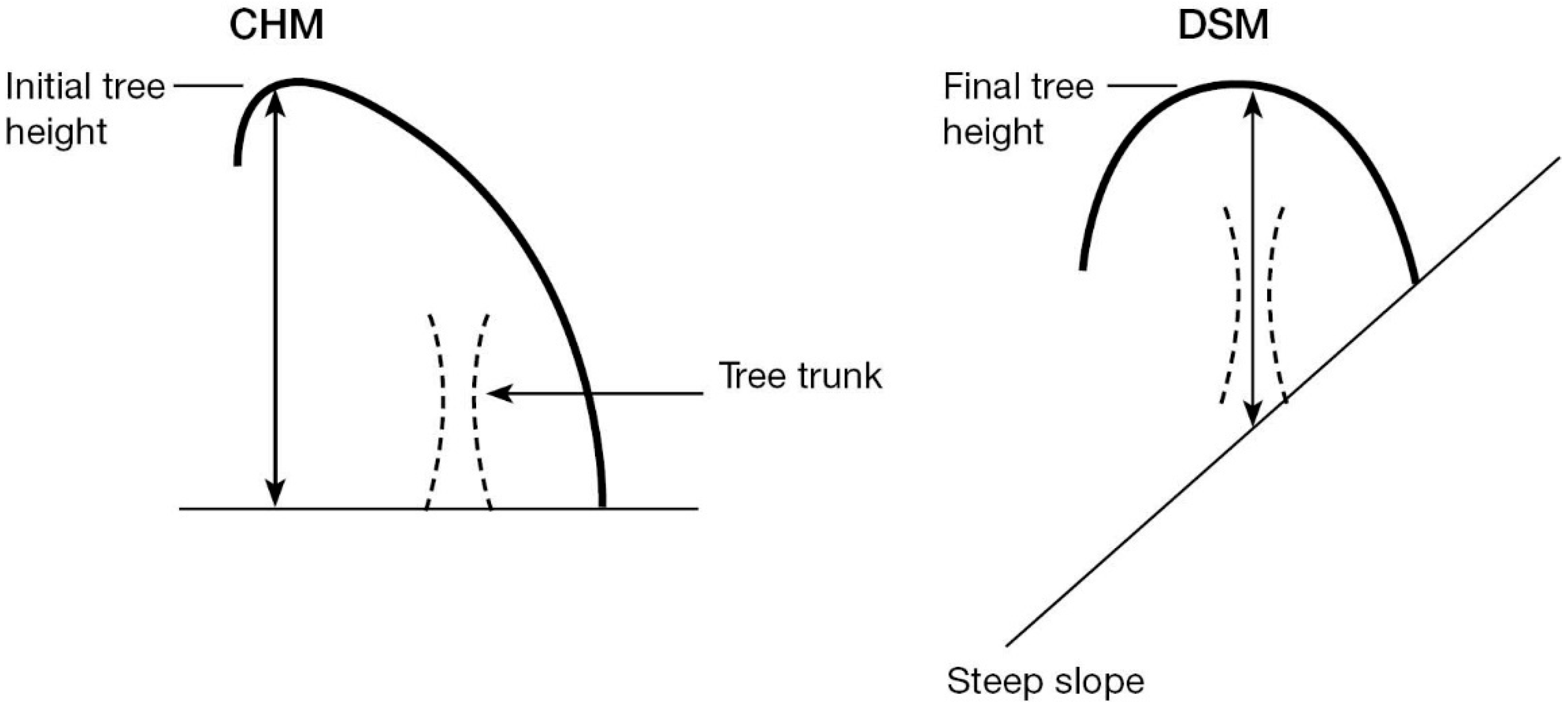
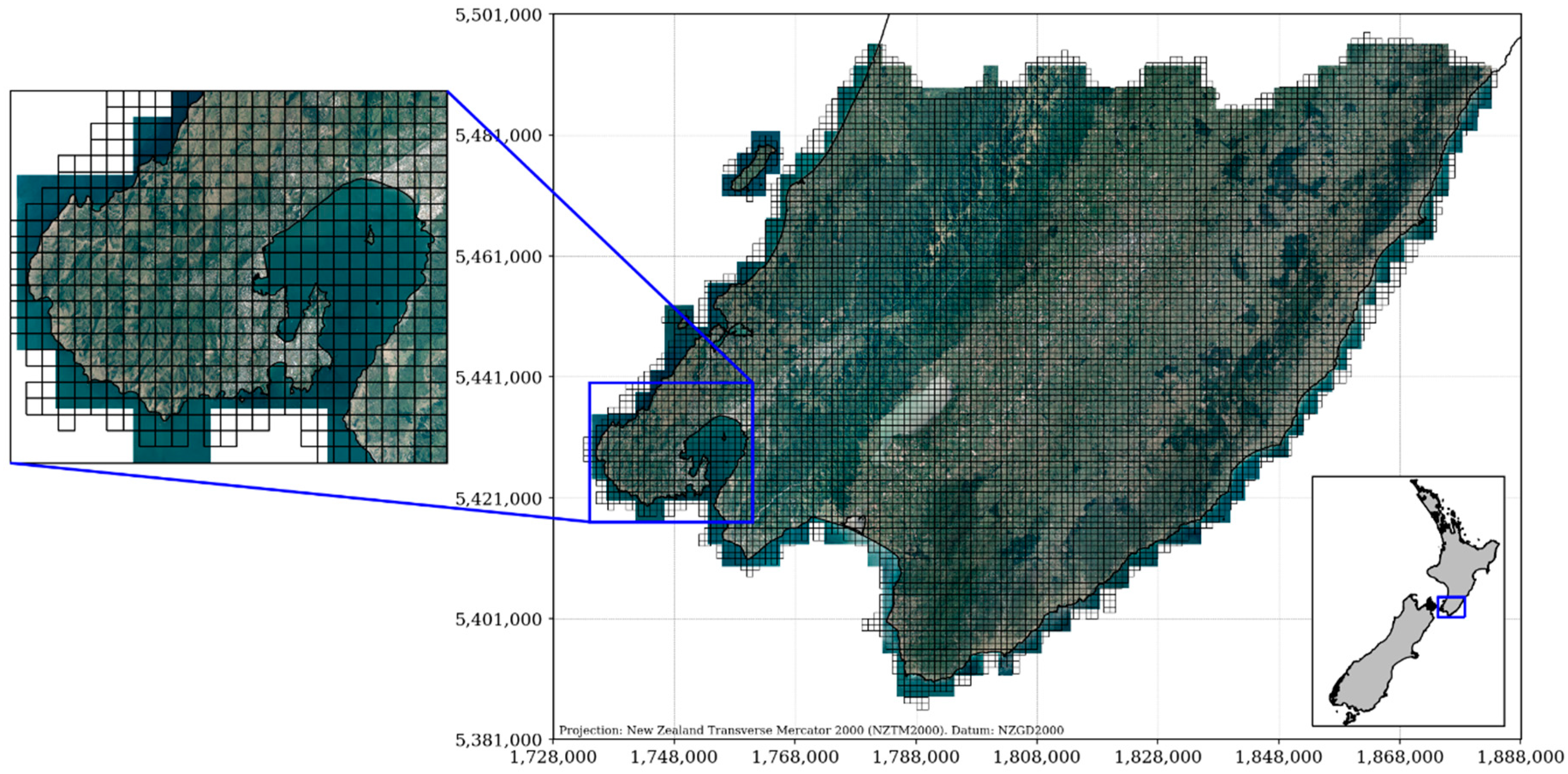
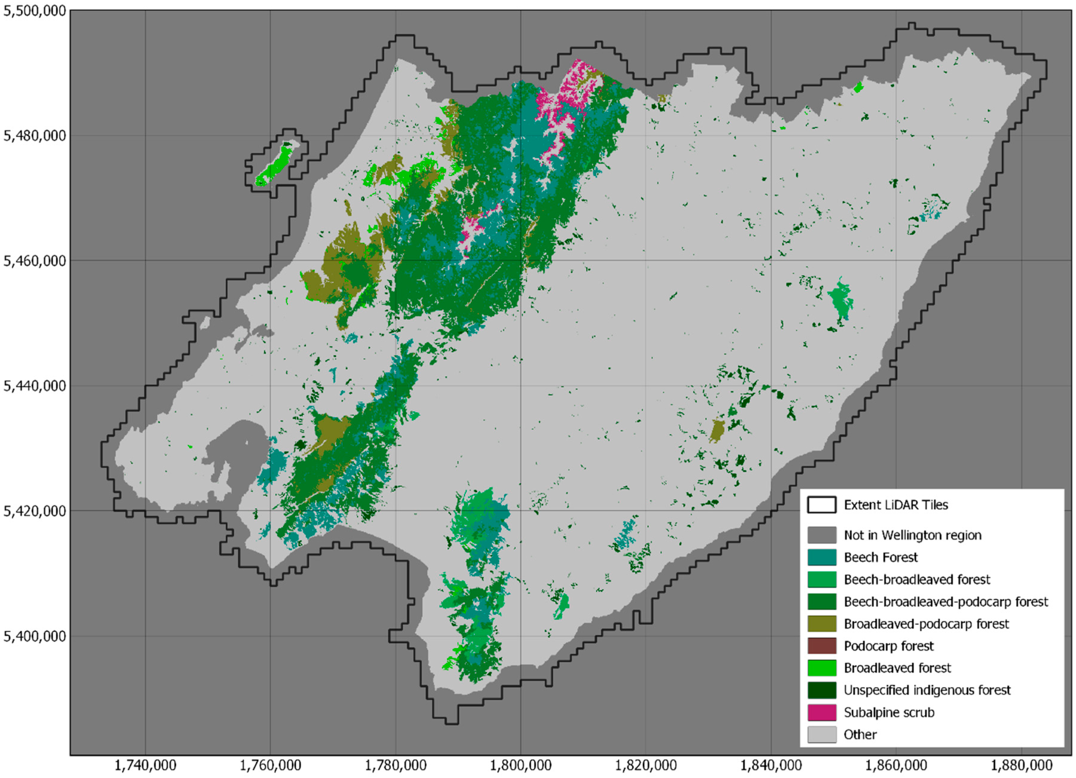
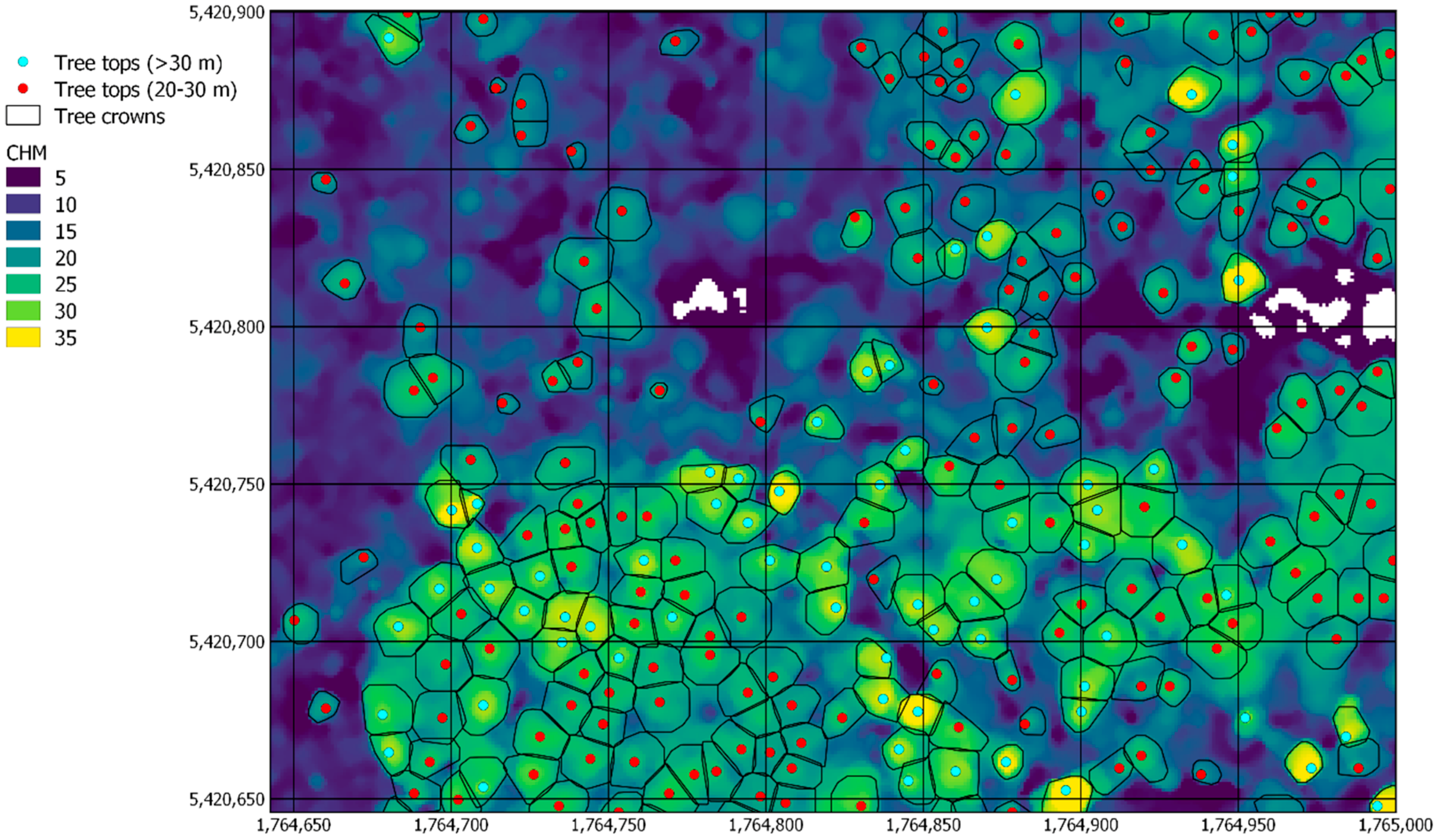
2. Materials and Methods
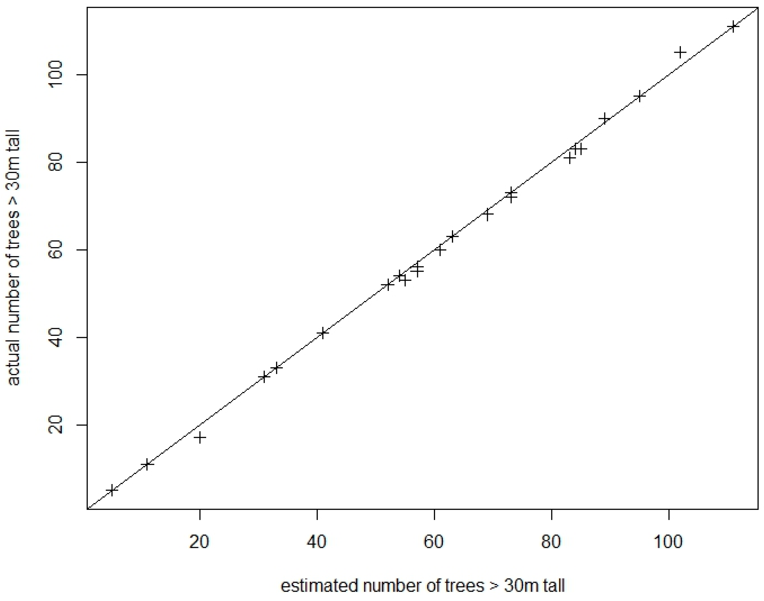
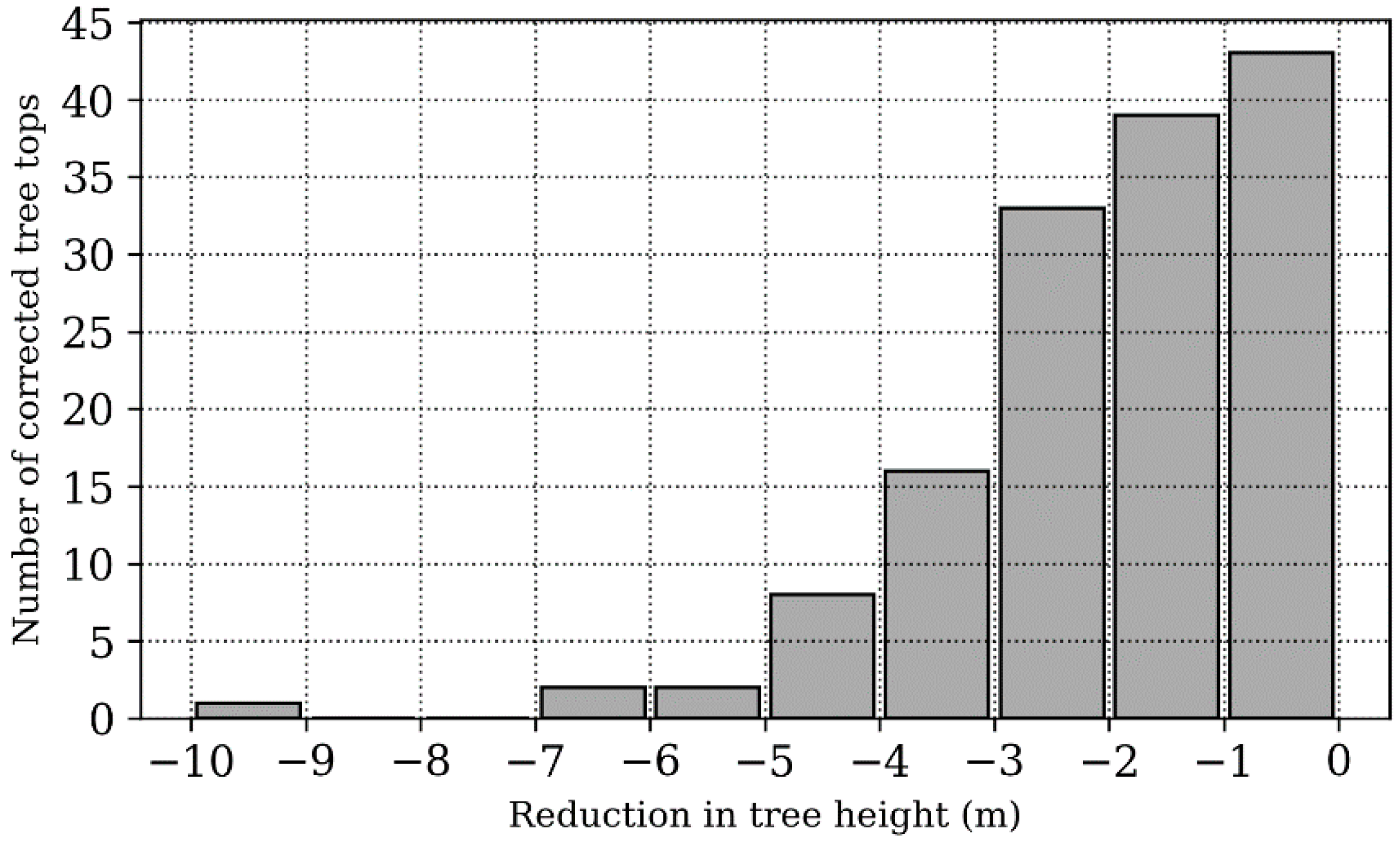
A LiDAR survey was conducted over the entire Wellington Region [45] primarily in early 2013 but with some additional aircraft flights later in 2013 and 2014, depending on weather. The LiDAR scanner was an Optech Airborne Laser Terrain Mapper ALTM 3100EA flown at a nominal height of 1000 m above the ground. Target point density was 1.7 ppsm with 50% swath overlap to ensure the minimum specification of 1.3 ppsm and a vertical accuracy of ±0.15 m. While these were the minimum requirements, the actual point density of the dataset ended up higher, ranging between 4–6 ppsm on average and >6 ppsm in regions with overlapping flight paths. Coincident with the LiDAR survey was an aerial photographic survey with blue, green, red and near-infrared bands, which was ortho-rectified to 30 cm pixels. The 1261 LiDAR flight lines of point cloud data were merged, tiled and further processed using the open-source LiDAR processing library, Sorted Pulse Data Software Library (SPDLib) [46].
The processing steps using SPDLib included: (i) removal of vertical noise, that is, undesired backscatter from atmospheric particles such as aerosols; (ii) 2-step classification of ground returns by applying the progressive morphology algorithm [47] first and the multiscale curvature algorithm [48] in the second step; (iii) definition of the height field within pulses and points by natural neighbor interpolation of the ground returns retrieving the absolute ground elevation; (iv) interpolation of ground and surface returns to a digital terrain model (DTM), digital surface model (DSM) and canopy height model (CHM) at 1 × 1 m pixel resolution using natural neighbor interpolation; and finally (v) removal of outliers in the CHM by applying a 5 × 5 m Gaussian median filter and screening out pixels below 0.5 m (undesired low vegetation) and above 60 m (erroneous high trees).
Individual trees were then identified from the CHM by finding the highest point in a 5 m circular moving window. If multiple pixels share the same CHM value, the center of mass of the pixel group is taken as the high point. These local maxima represent the tree top positions and the associated CHM value is extracted to define the tree top heights. During initial inspection using stereo mapping of the identified tree tops, it was found that some true tree top positions were different from the local maxima in the CHM if the tree was located in or close to steep terrain. This is the case, for instance, if the tree crown hangs over a cliff edge. The CHM-value assigned to the overhanging part of the crown is too high compared with the rest of the crown and the tree top height is thus overestimated. Figure 1 depicts an example scenario for a tree under such steep slope conditions. To account for this effect, we conducted a multi-step approach to identify a more realistic tree top position.
First, tree crowns were delineated based on an adapted version of the raster-based tree crown-growing algorithm by Dalponte and Coomes [28], using the local maxima as initial seeds. The original implementation from the R-package itcSegment [49] was ported Python code (optimized with Numba/Cython) and made publicly available as the PyCrown package [50]. It performs one order of magnitude faster than the C++ implementation from the R package for Airborne LiDAR Data Manipulation and Visualization for Forestry Applications (lidR) [51]. The idea behind the algorithm is that the crown grows around the initial seed considering a set of threshold values which are calculated based on four manually set parameters and the current tree information in each step: (i) the neighboring pixel is higher than seed height * 0.7; (ii) the neighboring pixel is higher than the mean height of current crown * 0.55; (iii) the neighboring pixel is below seed height * 1.05 and (iv) a maximum distance to the seed of 10 m (crown radius). We used standard settings from itcSegment and lidR except for parameter (i). The latter was raised from the standard 0.45 and set to 0.7 (which was also used by Dalponte and Coomes [28]) as inspection with aerial imagery revealed that many delineated tree crowns exceeded their actual radius. We did not choose parameters specific to individual tree species in order to keep a generic crown growing ruleset that is appropriate given that canopies comprise a mixture of species in these forests. We forced the algorithm to walk around the initial seed in a circular fashion with increasing distance in each iteration. This was necessary because the quadrilateral growing pattern in the original implementation lead to block-shaped tree crowns at the edges when the maximum crown radius is reached. After all tree crowns were delineated, a check was performed on whether the tree top location was too far (>1 standard deviation) down-slope compared with the mean ground elevation of its tree crown (i.e., mean DTM value). In such a case, the location of the highest point from the DSM was taken as the new tree top. In cases where the new high point of the DSM was too close to the border of the tree crown, the center of mass (COM) of the tree crown was selected.
The entire processing chain was run for a total of 9480 LiDAR tiles (each 1 × 1 km with 100 m overlap) of the Wellington Region on the NeSI high performance computer [52] and a spatial database of trees higher than 20 m was established, storing information on the tree top location, tree top height and tree crown shape; 3D tree shapefiles were exported. Figure 2 shows the study area overlaid with the individual LiDAR tiles.
Wiser et al. [53,54] used data from an extensive network of vegetation plots in New Zealand to objectively define a classification of forest alliances. Allen et al. [44] classified these into seven broad groups designated as beech forest, beech-broadleaved forest, beech-broadleaved-podocarp forest, broadleaved-podocarp forest, podocarp forest and other forests. An existing digital map of indigenous forest types, EcoSat Forests [55], was recoded according to Table 1 to produce a national map of forest alliance groups (“broadleaved forest” was added to the forest alliance groups to match the EcoSat Forest class “broadleaved forest”). This map was intersected with the shape file of tree top positions and heights obtained from our tree mapping algorithm to determine the number of tall trees within each forest alliance group. Intersection of tree positions and heights with a 15 m pixel DEM gave the density of tall trees within elevation ranges.
Assessing the accuracy of tall tree counting required three assumptions: (i) the CHM has a vertical random error of ±0.15 m (acquisition accuracy), no systematic error in the vertical and a small, random error component arising from spatial interpolation of the LiDAR points during the CHM generation (same order of magnitude as acquisition accuracy); (ii) the accuracy of identifying the tree top position by visually inspecting a stereo model of true color imagery (i.e., making use of the three dimensional view and color and textural differences between trees) is superior to the automated tree top identification using a local maximum filter; and (iii) manual analysis of stereo-imagery is more accurate at identifying tree top positions than ground-based techniques.
The accuracy assessment strategy does not try to validate the CHM itself but focuses on uncertainty in the geolocation of the automated tree mapping approach compared to a human pin-pointing the top of a tree using stereo vision. For validation of the CHM another independent measurement strategy is needed. This is typically conducted using ground-based measurements, which was beyond the scope of this study, as identifying overstory tree tops and estimating their heights from the ground in thick forest canopies is challenging and inherently uncertain. Therefore, we define the number of tall trees identified using stereo-imagery as the actual number of tall trees in absence of ground-based measurements.
We created stereo models of 25 permanent forest plots, using the raw digital aerial photographs, with stereo-analyst in Erdas Imagine [56] and compared the tree top position as identified by our algorithm to the visually perceived position in the stereo model. The tree height in both cases was taken from the CHM and compared. The forest plots are part of New Zealand’s Land Use and Carbon Analysis System (LUCAS), which is a national network of 20 × 20 m plots set up on an 8 km grid intersected on a map of indigenous vegetation [12]. The accuracy assessment was performed for intermediate-scale landforms (area ~10 ha), that is, land components of relatively uniform slope and aspect such as ridge crests, head slopes or foot slopes [57], surrounding the LUCAS plots. For each such land component, the number of tall trees (>30 m) delineated by our algorithm was compared to the number of tall trees determined visually from the stereo imagery.

3. Results

Figure 3 shows the spatial distribution of forest alliance groups in the Wellington Region and Table 2 gives areas of the forest alliance groups for the Wellington Region, for North and South Islands and for all New Zealand. In total there is 6.3 million ha of indigenous forest in New Zealand, some 23.9% of the land mass. The most common groups of forest alliances in New Zealand are beech forest, beech-broadleaved-podocarp forest and broadleaved-podocarp forest, in that order. In the Wellington Region these three groups are also the most common but with beech-broadleaved podocarp forest being the most common. Most of the indigenous forest in the Wellington Region is in the Tararua mountains, which form a south-west to north axis in the region. Broadleaved-podocarp forest is common at low altitudes on the western side of the Tararuas and typically progresses through beech-broadleaved-podocarp forest and then beech forest up altitudinal gradients. On the eastern side of the Tararuas the progression is simpler, starting at beech-broadleaved-podocarp forest with broadleaved-podocarp forest largely absent. In the Aorangi mountains in the south-east of the region, beech-broadleaved forest is the most common group.
The tree mapping algorithm was applied to the CHM of the entire Wellington Region, taking several hours on a high-performance computer. Figure 4 shows a small extract of the Wellington canopy height model and identified tree tops greater than 30 m tall. The number of tall trees over 30 m occurring in indigenous forest in the entire Wellington Region is estimated to be 286,041. Table 3 breaks these down into different height ranges. There are 53,029 trees over 35 m tall and 7340 giant trees over 40 m tall. The giant trees are mainly in the beech-broadleaved-podocarp and broadleaved-podocarp forests, corresponding to the presence of podocarps in these group. The density of giant trees in broadleaved-podocarp forest is three times that of beech-broadleaved-podocarp forest (Table 4). The tall trees between 30 and 35 m tall occur at sites with relatively high mean elevation in the beech forest (638 m) and low mean elevation in the broadleaved-podocarp forest (332 m) (Table 5).
In the stereo models, the 3-dimensional points representing tree tops were mostly located on the very tops of tall trees. Occasionally, where trees were very close to each other but were distinct in the stereo model due to different foliage color, only one tree top was identified in the canopy height model (i.e., a tree top was missed). This happened for 0.8% of the actual trees. Occasionally, where tree branches from the same tree were large and appeared to be separate trees, more than one tree top was identified (i.e., a tree top was added incorrectly). There was 1.6% of estimated tall trees added in this way. Figure 5 shows the number of tall trees identified using stereo-models (actual) versus the number of tall trees identified using the automated mapping approach (estimated). It shows that our automated tree top identification compares well with a manual approach using stereo-imagery—in absence of ground-based measurements—and can be used to count trees over large areas with a systematic error of about one percent (i.e., ≈(0.8–1.6)%).
In conjunction with the accuracy assessment of tree counting, we also tested the sensitivity of our automated mapping approach to varying inputs, that is, a CHM smoothed using different window sizes for the median filter and varying sizes of the local maximum filter to detect tall trees (Table 6). The number of trees detected is largest when a small window size is used, for example, 1081 tall trees using 3 m radius filters versus only 492 tall trees using 7 m radius filters. This reduction is caused by merging of trees and branches due to excessive smoothing of the CHM and by lower sensitivity to fine features in the CHM when using large filter sizes for the local peak detection.
Our tree mapping approach includes the automated correction of tree top positions in steep terrain. We noted for each individual tree whether its top position has been corrected or not and which correction method was used, that is, either the high point from the surface model within its crown or the center of mass of its crown. Analyzing the entire dataset of tall trees in Greater Wellington showed that about 3.1% of all tree tops have been corrected. Of these, 63.2% were corrected using the DSM and the remaining 36.8% using the COM method. We also calculated the reduction in tree height due to the correction procedure for one particular tile in mountainous terrain near the Totara Flats (index row: 82, column: 72, NZTM coordinates: 1,801,893:1,803,253 m and 5,466,814:5,468,104 m) (Figure 6). Of all trees detected in the 1 × 1 km tile, 145 had their height initially over-estimated, 13 of them by over 4 m. The average reduction in tree height following the correction method was −1.9 m and the maximum reduction was −9.4 m (for one tree on a cliff edge).

4. Discussion

This is the first time in New Zealand that a spatial tree inventory, where individual trees are labelled and heights recorded, has been achieved for an area as large as a region. This has produced unprecedented characterization of indigenous forests for which tree height information has previously been scant (the New Zealand Indigenous Carbon Monitoring System collected height data for 1304 trees nationally [58]). Our tree mapping algorithm was applied to the entire Wellington Region, taking only several hours on a high-performance computer. It identified over one million tall trees (>30 m) in the region, of which over a quarter of a million were in indigenous forest. Through evaluation of stereo-models of aerial photography, the algorithm was found to be accurate to within plus or minus one percent. Taking this uncertainty into account, the number of tall trees (>30 m) in the Wellington Region may be reported as 1,174,000 (±1%), of which 286,000 (±1%) are in indigenous forest.
While there are many tall trees in the Wellington Region, their density in the three most common forest alliance groups—beech, beech-broadleaved podocarp and broadleaved-podocarp—is relatively low at ~2 tall trees per hectare. The density, however, varies markedly with elevation and can reach over 10 trees per hectare in lowlands, reflecting the more equable climates including reduced wind strength. The relatively high density in three alliance groups containing podocarps is due to mature NZ conifers generally being more than twice as tall as mature broadleaved (angiosperm) trees [11]. In other alliance groups, tall angiosperm trees, such as Metrosideros umbellata and Knightia excelsa R.Br., have podocarp-like traits including thick, tough leaves and slow growth [11].
The spatial distribution of forest alliance groups is controlled by climate and soil [59] and by disturbance history, both natural, such as earthquakes, landslides and high winds and anthropogenic, such as fire and logging [60]. Broadleaved-podocarp forest is common at low altitudes on the western side of the Tararuas, where there is hill country with mild climate and consistent rainfall. Further into the mountainous Tararuas, hardy beech trees become more common due to the cold climate and strong prevailing westerly winds. Near the tree line, at about 1000 m, the forest is nearly all beech. On the eastern side of the Tararuas there is a narrower band of hill country between the mountains and the plains and so the elevation progression starts with beech-broadleaved podocarp forest, rather than broadleaved-podocarp forest. In the Aorangi mountains in the south-east of the region, beech-broadleaved forest is more common, than in the Tararuas, due to a more recent history of logging [61].
The accuracy assessment of the tree mapping algorithm for counting tall trees showed an overestimation by 1.6% due to incorrect separation of tree crowns and an underestimation by 0.8% due to incorrect merging of tree crowns. This implies a net systematic over-estimation of tree numbers by 0.8%, that is, 1.6%–0.8%. Rather than make a systematic downwards adjustment of 0.8% to all estimated tree numbers and estimating the uncertainty to which the adjustment can be determined (as in estimation of land cover areas from remote sensing [62]), we took a conservative approach and set the uncertainty to the required adjustment, rounded up to the nearest percent, that is, ±1%, giving a conservative range of 2% uncertainty, without actually making the adjustment. Not making a systematic adjustment to estimated tree numbers achieves the desirable property of being consistent with the individual tree inventory. Using stereoscopy of aerial photographs to check delineation of tall trees assumes that heights of the canopy in the CHM are accurate and that all uncertainty is due to finding tree top positions in the CHM. This avoided the difficulty of field measurement of tree heights in thick mountainous forests. For some lone tall trees on flat land we found that the CHM was indeed accurate to plus or minus 0.5 m, similar to that reported by Gatzioli et al. [63].
Coomes et al. [12] also identified biases in the number of segmented trees compared with ground-based field measurements (mainly of trees smaller than 30 m). They found that the CHM-based tree mapping algorithm was sensitive to the tree height—strongly under-estimating the number of short understory trees (<12 m) and over-estimating the number of taller trees (>12 m) by 16% (subdivision of single overstory trees). However, identifying tree tops from the ground, especially of overstory trees, is challenging in thick forest canopies. Based on these previous findings we carefully evaluated settings to minimize uncertainties arising from both the incorrect separation and merging of tree crowns.
The choice of parameters of the tree mapping algorithm not only affects the number of trees detected but also the identified tree-top height. Three parameters most affect the results: the pixel resolution of the raster data sets (CHM, DSM and DTM); the window size of the smoothing filter for the CHM; and the maximum filter for the tree top detection. Our accuracy assessment revealed that, on the one hand, in 0.8% of the cases two trees were too close together to be detected as two separate trees by a 5 × 5 m median filter and 5 × 5 m maximum filter. This suggests a smaller window size (e.g., 3 × 3 m) would be beneficial in detecting more trees. On the other hand, about 1.6% of tall trees appeared to be separate trees because tree branches from the same tree were very large. This suggests a larger window size (e.g., 7 × 7 m) would be beneficial in detecting fewer trees. This is supported by our sensitivity analysis which showed both the effects of merging of trees due to excessive smoothing of the CHM and a lower sensitivity for tree top detection using too large window sizes.
We also tested the effect of a higher resolution CHM (0.5 × 0.5 m pixels) on the identified number of tall trees but found that almost identical results could be achieved with a 1 × 1 m pixel resolution and small window sizes for the smoothing and local maxima identification. We conclude that the overall number of trees using our set of parameters is accurate and the two contrasting effects balance each other out on a large-scale data set. However, we note that for an accurate local analysis, the set of parameters should be adjusted to the local canopy structure and properties.
Application of the algorithm in a region with steep landscapes, such as the Wellington Region, is made possible by the check and correction for over-estimated heights of trees on steep terrain. In a 1 × 1 km LiDAR tile containing typically mountainous terrain, 145 trees had their height initially over-estimated by 1.9 m on average; of these, 13 were overestimated by more than four meters. This would have introduced errors for many trees if the check and correction had not been applied. Previous studies reported similar reductions in tree top height following the correction of the terrain-effect. Khosravipour et al. [38] observed an average reduction of about 0.4 m and maximum reductions of 1.8 m of pine trees in the French Alps. Alexander et al. [40] conducted a research study in the tropical forest in Sumatra and found differences of 16.6 m in tree heights estimated from the CHM and DSM. Our findings are consistent with these previous efforts and we present a flexible and fast method to correct for the terrain-effect on a large-scale LiDAR dataset, which has not been done before and consider tree specific parameters such as the crown shape.
A source of error for estimated tree height that we did not consider correcting is tree lean. On steep slopes it is possible that trees may lean preferentially downhill. We did not see any evidence in the stereo models of tree lean in the tall indigenous trees on steep slopes, however, researchers have found systematic tree lean elsewhere. Gatziolis et al. [63] found that trees on steep slopes in the US Pacific Northwest had a mean offset of about 1 m horizontal between base and top of tree. A 1 m offset for a tall tree on a 20 degree slope would result in a small overestimation of tree height by 0.4 m, so should not have a significant impact on the statistics of tree heights. In extreme cases when the offset is 5 m, the tree height would be overestimated by about 1.5 m. This represents a possible, or maximum, error of plus 5% for tree heights on steep slopes.
While the tree-mapping algorithm took several hours for the Wellington Region, the processing of the raw LiDAR point cloud data to DTMs/DSMs/CHMs took much longer. The LiDAR data were divided into 9480 tiles of 1 km2, with each one taking several hours to process on the high-performance computer in 2014—when we first processed the dataset. Now, the processing time has reduced to less than 30 min per tile and can be conveniently parallelized by taking advantage of modern cluster computing systems. While the preparation of the data represents a significant investment in time and compute resources, it only has to be done once and there are many other uses of the LiDAR-derived data in addition to forest characterization, such as ecological modelling [64], flood control [65] and roading. Indeed, several more regional authorities in New Zealand are currently acquiring or planning regional LiDAR surveys, including the Gisborne district, Northland Regional Council and Hawke’s Bay Regional Council. (The Bay of Plenty already has regional LiDAR coverage, as does Wellington.) To coordinate a national approach to LiDAR acquisition, Land Information New Zealand has brought out a base specification [66] providing a foundation for public sector LiDAR data procurement.
The map of forest alliance groups is based on a previously existing map of indigenous forests, EcoSat Forests. This 1:50,000 scale database was derived by combining the vegetation layer in New Zealand Land Resource Inventory (NZLRI [67]) with the Land Cover Database (LCDB). In the 1:50,000 scale NZLRI, the area of indigenous forest types within landform polygons was estimated from a combination of fieldwork and photointerpretation of stereo aerial photographs. The nominal date of the mapping is 1980. The LCDB has a higher spatial resolution with a minimum mapping unit of 1 ha and a later currency with mapping dates of 1995, 2001–2002, 2008 and 2012; however, it has lower thematic resolution with only two indigenous forest classes. EcoSat Forests combines the two databases in a way that takes advantage of the high thematic resolution of NZLRI with the high spatial resolution of LCDB but this assumes that there has been little change in the indigenous forest classes since 1980. Indeed, the main forest alliance groups are unlikely to have changed since 1980 but as the accuracy of the NZLRI indigenous forest class mapping is not well characterized, the map of forest alliance groups used here should be considered a preliminary version only. Nevertheless, we believe the general spatial patterns of forest alliance groups as reported in this paper are well represented. Work is underway to produce a more current national map of forest alliance groups by integrating recent satellite imagery with recently surveyed forest plots.
Our tree inventory provides a useful baseline and starting point for monitoring the condition of indigenous forests in New Zealand. If diseases, such as kauri dieback and myrtle rust, spread through indigenous forests in New Zealand, then the impact on individual trees could be assessed and recorded. There is also the expectation of an increasing frequency and intensity of natural disturbances under climate change and continuing damage from mammalian pests. Certainly, tree mortality can be determined through repeat LiDAR surveys and possibly deteriorating condition could be assessed through repeated hyperspectral surveys [68]. Furthermore, the tree inventory lays the foundation for future work such as modelling the spatial distribution of tall trees in the landscape and investigating the underlying drivers governing their distribution.

5. Conclusions

Region-wide tree inventories can significantly improve characterization of natural forests and provide a useful baseline for monitoring conditions. It is possible to derive region-wide models of forest canopy height from LiDAR at reasonable cost. From the CHM it is further possible to derive a region-wide inventory of tall trees. Our tree top detection and correction scheme, which identifies tree tops from local maxima in the CHM and uses the DSM and DTM to correct for terrain-effects, provides a simple and fast method to accurately map overstory trees in flat as well as mountainous areas. It can be directly applied to improve existing and build new tree inventories in regions where LiDAR data is available.
The number of tall trees over 30 m in the Wellington Region was estimated to be 286,041 (±1%) and the number of giant trees over 40 m was estimated to be 7340 (±1%). The giant trees were found mainly in broadleaved-podocarp forest (density = 0.12 trees/ha) and beech-broadleaved-podocarp forest (density = 0.04 trees/ha).

Author Contributions

J.Z., conceptualization, methodology, formal analysis, software implementation, writing and editing; J.R.D., conceptualization, methodology, validation, writing and editing; J.D.S., conceptualization and methodology; S.K.W. reviewing and editing; B.J., formal analysis.

Funding

The Ministry of Business Innovation & Employment funded this research under contract C09X1709.

Acknowledgments

We would like to thank David Pairman from Landcare Research for the fruitful discussions and internal review.

Conflicts of Interest

The authors declare no conflict of interest.

References

  1. Dymond, J.R.; Shepherd, J.D.; Newsome, P.F.; Belliss, S. Estimating change in areas of indigenous vegetation cover in New Zealand from the New Zealand Land Cover Database (LCDB). N. Z. J. Ecol. 2017, 41. [Google Scholar] [CrossRef] [Green Version]
  2. Dymond, J.R.; Ausseil, A.-G.E.; Peltzer, D.A.; Herzig, A. Conditions and trends of ecosystem services in New Zealand—A synopsis. Solut. J. 2014, 5, 38–45. [Google Scholar]
  3. Wardle, P. Vegetation of New Zealand; Cambridge University Press: Cambridge, UK, 1991; ISBN 9780521258739. [Google Scholar]
  4. Díaz, I.A.; Sieving, K.E.; Peña-Foxon, M.E.; Larraín, J.; Armesto, J.J. Epiphyte diversity and biomass loads of canopy emergent trees in Chilean temperate rain forests: A neglected functional component. For. Ecol. Manag. 2010, 259, 1490–1501. [Google Scholar] [CrossRef]
  5. Dislich, R.; Mantovani, W. Vascular epiphyte assemblages in a Brazilian Atlantic Forest fragment: Investigating the effect of host tree features. Plant Ecol. 2016, 217. [Google Scholar] [CrossRef]
  6. Li, S.; Liu, S.; Shi, X.-M.; Liu, W.-Y.; Song, L.; Lu, H.-Z.; Chen, X.; Wu, C.-S. Forest Type and Tree Characteristics Determine the Vertical Distribution of Epiphytic Lichen Biomass in Subtropical Forests. Forests 2017, 8, 436. [Google Scholar] [CrossRef]
  7. Lesak, A.A.; Radeloff, V.C.; Hawbaker, T.J.; Pidgeon, A.M.; Gobakken, T.; Contrucci, K. Modeling forest songbird species richness using LiDAR-derived measures of forest structure. Remote Sens. Environ. 2011, 115, 2823–2835. [Google Scholar] [CrossRef]
  8. Flaspohler, D.J.; Giardina, C.P.; Asner, G.P.; Hart, P.; Price, J.; Lyons, C.K.; Castaneda, X. Long-term effects of fragmentation and fragment properties on bird species richness in Hawaiian forests. Biol. Conserv. 2010, 143, 280–288. [Google Scholar] [CrossRef]
  9. Greene, D.F.; Johnson, E.A. A Model of Wind Dispersal of Winged or Plumed Seeds. Ecology 1989, 70, 339–347. [Google Scholar] [CrossRef]
  10. Loehle, C. Strategy Space and the Disturbance Spectrum: A Life-History Model for Tree Species Coexistence. Am. Nat. 2000, 156, 14–33. [Google Scholar] [CrossRef] [PubMed]
  11. McGlone, M.S.; Richardson, S.J.; Jordan, G.J. Comparative biogeography of New Zealand trees: Species richness, height, leaf traits and range sizes. N. Z. J. Ecol. 2010, 34, 137–151. [Google Scholar]
  12. Coomes, D.A.; Šafka, D.; Shepherd, J.; Dalponte, M.; Holdaway, R. Airborne laser scanning of natural forests in New Zealand reveals the influences of wind on forest carbon. For. Ecosyst. 2018, 5, 10. [Google Scholar] [CrossRef]
  13. Koukoulas, S.; Blackburn, G.A. Mapping individual tree location, height and species in broadleaved deciduous forest using airborne LIDAR and multi-spectral remotely sensed data. Int. J. Remote Sens. 2005, 26, 431–455. [Google Scholar] [CrossRef]
  14. Latifi, H.; Nothdurft, A.; Koch, B. Non-parametric prediction and mapping of standing timber volume and biomass in a temperate forest: Application of multiple optical/LiDAR-derived predictors. Forestry 2010, 83, 395–407. [Google Scholar] [CrossRef]
  15. O’Neil-Dunne, J.; MacFaden, S.; Royar, A. A Versatile, Production-Oriented Approach to High-Resolution Tree-Canopy Mapping in Urban and Suburban Landscapes Using GEOBIA and Data Fusion. Remote Sens. 2014, 6, 12837–12865. [Google Scholar] [CrossRef] [Green Version]
  16. McPherson, E.G.; Simpson, J.R.; Xiao, Q.; Wu, C. Million trees Los Angeles canopy cover and benefit assessment. Landsc. Urban Plan. 2011, 99, 40–50. [Google Scholar] [CrossRef]
  17. Crowther, T.W.; Glick, H.B.; Covey, K.R.; Bettigole, C.; Maynard, D.S.; Thomas, S.M.; Smith, J.R.; Hintler, G.; Duguid, M.C.; Amatulli, G.; et al. Mapping tree density at a global scale. Nature 2015, 525, 201–205. [Google Scholar] [CrossRef] [PubMed]
  18. Lefsky, M.A.; Cohen, W.B.; Acker, S.A.; Parker, G.G.; Spies, T.A.; Harding, D. Lidar Remote Sensing of the Canopy Structure and Biophysical Properties of Douglas-Fir Western Hemlock Forests. Remote Sens. Environ. 1999, 70, 339–361. [Google Scholar] [CrossRef]
  19. Hyyppä, J.; Kelle, O.; Lehikoinen, M.; Inkinen, M. A segmentation-based method to retrieve stem volume estimates from 3-D tree height models produced by laser scanners. IEEE Trans. Geosci. Remote Sens. 2001, 39, 969–975. [Google Scholar] [CrossRef]
  20. Zhen, Z.; Quackenbush, L.; Zhang, L. Trends in Automatic Individual Tree Crown Detection and Delineation—Evolution of LiDAR Data. Remote Sens. 2016, 8, 333. [Google Scholar] [CrossRef]
  21. Ayrey, E.; Fraver, S.; Kershaw, J.A.; Kenefic, L.S.; Hayes, D.; Weiskittel, A.R.; Roth, B.E. Layer Stacking: A Novel Algorithm for Individual Forest Tree Segmentation from LiDAR Point Clouds. Can. J. Remote Sens. 2017, 43, 16–27. [Google Scholar] [CrossRef]
  22. Hamraz, H.; Contreras, M.A.; Zhang, J. A robust approach for tree segmentation in deciduous forests using small-footprint airborne LiDAR data. Int. J. Appl. Earth Obs. Geoinf. 2016, 52, 532–541. [Google Scholar] [CrossRef] [Green Version]
  23. Duncanson, L.I.; Cook, B.D.; Hurtt, G.C.; Dubayah, R.O. An efficient, multi-layered crown delineation algorithm for mapping individual tree structure across multiple ecosystems. Remote Sens. Environ. 2014, 154, 378–386. [Google Scholar] [CrossRef]
  24. Bunting, P.; Lucas, R. The delineation of tree crowns in Australian mixed species forests using hyperspectral Compact Airborne Spectrographic Imager (CASI) data. Remote Sens. Environ. 2006, 101, 230–248. [Google Scholar] [CrossRef]
  25. Wang, Y.; Hyyppa, J.; Liang, X.; Kaartinen, H.; Yu, X.; Lindberg, E.; Holmgren, J.; Qin, Y.; Mallet, C.; Ferraz, A.; et al. International Benchmarking of the Individual Tree Detection Methods for Modeling 3-D Canopy Structure for Silviculture and Forest Ecology Using Airborne Laser Scanning. IEEE Trans. Geosci. Remote Sens. 2016, 54, 5011–5027. [Google Scholar] [CrossRef]
  26. Li, W.; Guo, Q.; Jakubowski, M.K.; Kelly, M. A New Method for Segmenting Individual Trees from the Lidar Point Cloud. Photogramm. Eng. Remote Sens. 2012, 78, 75–84. [Google Scholar] [CrossRef]
  27. Pirotti, F.; Kobal, M.; Roussel, J.R. A comparison of tree segmentation methods using very high density airborne laser scanner data. Int. Arch. Photogramm. Remote Sens. Spat. Inf. Sci. 2017, 42, 285–290. [Google Scholar] [CrossRef]
  28. Dalponte, M.; Coomes, D.A. Tree-centric mapping of forest carbon density from airborne laser scanning and hyperspectral data. Methods Ecol. Evol. 2016, 7, 1236–1245. [Google Scholar] [CrossRef] [PubMed] [Green Version]
  29. Fonstad, M.A.; Dietrich, J.T.; Courville, B.C.; Jensen, J.L.; Carbonneau, P.E. Topographic structure from motion: A new development in photogrammetric measurement. Earth Surf. Process. Landf. 2013, 38, 421–430. [Google Scholar] [CrossRef]
  30. Baltsavias, E.; Gruen, A.; Eisenbeiss, H.; Zhang, L.; Waser, L.T. High-quality image matching and automated generation of 3D tree models. Int. J. Remote Sens. 2008, 29, 1243–1259. [Google Scholar] [CrossRef]
  31. White, J.; Wulder, M.; Vastaranta, M.; Coops, N.; Pitt, D.; Woods, M. The Utility of Image-Based Point Clouds for Forest Inventory: A Comparison with Airborne Laser Scanning. Forests 2013, 4, 518–536. [Google Scholar] [CrossRef] [Green Version]
  32. St-Onge, B.; Jumelet, J.; Cobello, M.; Véga, C. Measuring individual tree height using a combination of stereophotogrammetry and lidar. Can. J. For. Res. 2004, 34, 2122–2130. [Google Scholar] [CrossRef]
  33. Dandois, J.P.; Ellis, E.C. Remote Sensing of Vegetation Structure Using Computer Vision. Remote Sens. 2010, 2, 1157–1176. [Google Scholar] [CrossRef] [Green Version]
  34. Westoby, M.J.; Brasington, J.; Glasser, N.F.; Hambrey, M.J.; Reynolds, J.M. ‘Structure-from-Motion’ photogrammetry: A low-cost, effective tool for geoscience applications. Geomorphology 2012, 179, 300–314. [Google Scholar] [CrossRef] [Green Version]
  35. Brandtberg, T.; Warner, T.A.; Landenberger, R.E.; McGraw, J.B. Detection and analysis of individual leaf-off tree crowns in small footprint, high sampling density lidar data from the eastern deciduous forest in North America. Remote Sens. Environ. 2003, 85, 290–303. [Google Scholar] [CrossRef]
  36. Hirata, Y. The effects of footprint size and sampling density in airborne laser scanning to extract individual trees in mountainous terrain. Int. Arch. Photogramm. Remote Sens. Spat. Inf. Sci. 2004, 36, 102–107. [Google Scholar]
  37. Hansen, E.; Ene, L.; Gobakken, T.; Ørka, H.; Bollandsås, O.; Næsset, E. Countering Negative Effects of Terrain Slope on Airborne Laser Scanner Data Using Procrustean Transformation and Histogram Matching. Forests 2017, 8, 401. [Google Scholar] [CrossRef]
  38. Khosravipour, A.; Skidmore, A.K.; Wang, T.; Isenburg, M.; Khoshelham, K. Effect of slope on treetop detection using a LiDAR Canopy Height Model. ISPRS J. Photogramm. Remote Sens. 2015, 104, 44–52. [Google Scholar] [CrossRef]
  39. Duan, Z.; Zhao, D.; Zeng, Y.; Zhao, Y.; Wu, B.; Zhu, J. Assessing and Correcting Topographic Effects on Forest Canopy Height Retrieval Using Airborne LiDAR Data. Sensors 2015, 15, 12133–12155. [Google Scholar] [CrossRef] [PubMed] [Green Version]
  40. Alexander, C.; Korstjens, A.H.; Hill, R.A. Influence of micro-topography and crown characteristics on tree height estimations in tropical forests based on LiDAR canopy height models. Int. J. Appl. Earth Obs. Geoinf. 2018, 65, 105–113. [Google Scholar] [CrossRef]
  41. Regional High-Resolution DEM Now on LDS, Wellington Regional Government GIS Group (2016). Available online: http://mapping.gw.govt.nz/News06.htm (accessed on 3 October 2018).
  42. Coomes, D.A.; Dalponte, M.; Jucker, T.; Asner, G.P.; Banin, L.F.; Burslem, D.F.R.P.; Lewis, S.L.; Nilus, R.; Phillips, O.L.; Phua, M.-H.; et al. Area-based vs tree-centric approaches to mapping forest carbon in Southeast Asian forests from airborne laser scanning data. Remote Sens. Environ. 2017, 194, 77–88. [Google Scholar] [CrossRef]
  43. Kandare, K.; Dalponte, M.; Ørka, H.; Frizzera, L.; Næsset, E. Prediction of Species-Specific Volume Using Different Inventory Approaches by Fusing Airborne Laser Scanning and Hyperspectral Data. Remote Sens. 2017, 9, 400. [Google Scholar] [CrossRef]
  44. Allen, R.B.; Bellingham, P.J.; Holdaway, R.J.; Wiser, S.K. New Zealand’s indigenous forests and shrublands. In Ecosystem Services in New Zealand—Conditions and Trends; Dymond, J.R., Ed.; Manaaki Whenua Press: Lincoln, New Zealand, 2013; pp. 34–48. ISBN 9780478347364. [Google Scholar]
  45. Müller, M.U.; Shepherd, J.D.; Dymond, J.R. Support vector machine classification of woody patches in New Zealand from synthetic aperture radar and optical data, with LiDAR training. J. Appl. Remote Sens. 2015, 9, 095984. [Google Scholar] [CrossRef] [Green Version]
  46. Bunting, P.; Armston, J.; Clewley, D.; Lucas, R. The sorted pulse data software library (SPDLib): Open source tools for processing LiDAR data. In Proceedings of the SilviLaser 2011, 11th International Conference on LiDAR Applications for Assessing Forest Ecosystems, University of Tasmania, Hobart, Australia, 16–20 October 2011; pp. 1–11. [Google Scholar]
  47. Zhang, K.; Chen, S.; Whitman, D.; Shyu, M.; Yan, J.; Zhang, C. A progressive morphological filter for removing nonground measurements from airborne LiDAR data. IEEE Trans. Geosci. Remote Sens. 2003, 41, 872–882. [Google Scholar] [CrossRef]
  48. Evans, J.S.; Hudak, A.T. A Multiscale Curvature Algorithm for Classifying Discrete Return LiDAR in Forested Environments. IEEE Trans. Geosci. Remote Sens. 2007, 45, 1029–1038. [Google Scholar] [CrossRef] [Green Version]
  49. Dalponte, M. itcSegment: Individual Tree Crowns Segmentation. R Package Version 0.8. Available online: https://CRAN.R-project.org/package=itcSegment (accessed on 3 October 2018).
  50. Zörner, J.; Dymond, J.; Shepherd, J.; Jolly, B. PyCrown-Fast Raster-Based Individual Tree Segmentation for LiDAR Data; Landcare Research Ltd.: Lincoln, New Zealand, 2018. [Google Scholar] [CrossRef]
  51. Roussel, J.-R.; Auty, D. lidR: Airborne LiDAR Data Manipulation and Visualization for Forestry Applications. R Package Version 1.5.1. Available online: https://CRAN.R-project.org/package=lidR (accessed on 3 October 2018).
  52. NeSI Pan Cluster, Centre for eResearch. Available online: https://wiki.auckland.ac.nz/display/CER/NeSI+Pan+Cluster (accessed on 3 October 2018).
  53. Wiser, S.; Thomson, F.; de Cáceres, M. Expanding an existing classification of New Zealand vegetation to include non-forested vegetation. N. Z. J. Ecol. 2016, 40, 160–178. [Google Scholar] [CrossRef] [Green Version]
  54. Wiser, S.K.; de Cáceres, M. New Zealand’s plot-based classification of vegetation. Phytocoenologia 2018, 48, 153–161. [Google Scholar] [CrossRef]
  55. Shepherd, J.D.; Ausseil, A.-G.; Dymond, J.R. EcoSat Forests: A 1:750,000 Scale Map of Indigenous Forest Classes in New Zealand; Manaaki Whenua Press: Lincoln, New Zealand, 2005; Available online: https://lris.scinfo.org.nz/ (accessed on 3 October 2018).
  56. Erdas Imagine, Hexagon Geospatial. Available online: https://www.hexagongeospatial.com (accessed on 3 October 2018).
  57. Dymond, J.R.; Derose, R.C.; Harmsworth, G.R. Automated mapping of land components from digital elevation data. Earth Surf. Process. Landf. 1995, 20, 131–137. [Google Scholar] [CrossRef]
  58. Bellingham, P.; Wiser, S.; Coomes, D.; Dunningham, A. Review of Permanent Plots for Long-Term Monitoring of New Zealand’s Indigenous Forests; Science for Conservation; Department of Conservation: Wellington, New Zealand, 2000; ISBN 9780478219586.
  59. Leathwick, J.; Wilson, G.; Rutledge, D.; Wardle, P.; Morgan, F.; Johnston, K.; McLeod, M.; Kirkpatrick, R. Land Environments of New Zealand; David Bateman Ltd.: Auckland, New Zealand, 2003; ISBN 9781869535223. [Google Scholar]
  60. Wardle, P. Facets of the distribution of forest vegetation in New Zealand. N. Z. J. Bot. 1964, 2, 352–366. [Google Scholar] [CrossRef] [Green Version]
  61. Ministry for Culture and Heritage. Te Ara: The Encyclopaedia of New Zealand. Available online: https://teara.govt.nz/en/logging-native-forests/page-1 (accessed on 3 October 2018).
  62. Dymond, J.R.; Shepherd, J.D.; Newsome, P.F.; Gapare, N.; Burgess, D.W.; Watt, P. Remote sensing of land-use change for Kyoto Protocol reporting: The New Zealand case. Environ. Sci. Policy 2012, 16, 1–8. [Google Scholar] [CrossRef]
  63. Gatziolis, D.; Fried, J.S.; Monleon, V.S. Challenges to estimating tree height via LiDAR in closed-canopy forests: A parable from Western Oregon. For. Sci. 2010, 56, 139–155. [Google Scholar]
  64. Vierling, K.T.; Vierling, L.A.; Gould, W.A.; Martinuzzi, S.; Clawges, R.M. Lidar: Shedding new light on habitat characterization and modeling. Front. Ecol. Environ. 2008, 6, 90–98. [Google Scholar] [CrossRef]
  65. Turner, A.; Colby, J.; Csontos, R.; Batten, M. Flood Modeling Using a Synthesis of Multi-Platform LiDAR Data. Water 2013, 5, 1533–1560. [Google Scholar] [CrossRef] [Green Version]
  66. New Zealand National Aerial LiDAR Base Specification, Version 1.1. 2018. Available online: https://www.linz.govt.nz/system/files_force/media/doc/loci_nz-national-aerial-lidar-base-specification_20180629.pdf (accessed on 3 October 2018).
  67. The New Zealand Land Resource Inventory. Available online: https://lris.scinfo.org.nz/layer/48055-nzlri-vegetation/ (accessed on 3 October 2018).
  68. Asner, G.P.; Martin, R.E.; Keith, L.M.; Heller, W.P.; Hughes, M.A.; Vaughn, N.R.; Hughes, R.F.; Balzotti, C. A Spectral Mapping Signature for the Rapid Ohia Death (ROD) Pathogen in Hawaiian Forests. Remote Sens. 2018, 10, 404. [Google Scholar] [CrossRef]
Figure 1. Sketch of initial tree top position as derived from the CHM (canopy height model) using local maxima filtering (left panel) and new tree top position (right panel) defined as the highest point in the DSM (digital surface model) within the tree crown boundary minus the DTM (digital terrain model).
Forests 09 00702 g001
Figure 2. The Wellington Region of New Zealand and the mosaic of aerial photographs taken during the LiDAR survey in 2013 and 2014. The LiDAR data is subdivided into an equally-spaced grid of 9480 tiles with a 1 × 1 km spacing (outlined in black). Map projection is New Zealand Transverse Mercator (NZTM).
Forests 09 00702 g002
Figure 3. Spatial distribution of forest alliance groups in the Wellington Region. Most indigenous forests are in the Tararua mountains which form a north to south-west axis. Most of remaining indigenous forests are in Aorangi mountains in the southernmost part of region. Map projection is NZTM.
Forests 09 00702 g003
Figure 4. Extract of the canopy height model in the Wellington Region and identified tree tops greater than 30 m tall (cyan) and between 20 and 30 m tall (red). Map projection is NZTM.
Forests 09 00702 g004
Figure 5. Number of tall trees within each land component as identified in stereo-imagery (actual) versus the number of tall trees as identified by the automated tree mapping algorithm (estimated).
Forests 09 00702 g005
Figure 6. Effect of the automated tree top correction method on the estimated tree top height. Trees situated on steep slopes or overhanging a cliff edge typically have their top height overestimated due to the terrain normalization of the DSM. Most tree tops are reduced by 1 to 4.
Forests 09 00702 g006
Table 1. Table for recoding EcoSat forest class to forest alliance group.
Forest Alliance GroupEcoSat Forests Classes
Beech forestBeech forest
Beech-broadleaved forestBeech-broadleaved forest
Beech-broadleaved podocarp forestPodocarp-broadleaved/Beech forest
Beech/Podocarp-broadleaved forest
Broadleaved-podocarp forestPodocarp-broadleaved forest
Kauri forest
Podocarp forestPodocarp forest
Broadleaved forestBroadleaved forest
Coastal forest
Unspecified indigenous forestUnspecified indigenous forest
Table 2. Areas in hectares of forest alliance groups in the Wellington Region, North Island, South Island and New Zealand.
Forest Alliance GroupWellingtonNorth IslandSouth IslandNew Zealand
Beech forest37,402360,1041,826,9402,187,044
Beech-broadleaved forest794628,70369,60698,309
Beech-broadleaved podocarp forest81,155685,9521,148,2421,834,194
Broadleaved-podocarp forest17,341891,306447,8231,339,129
Podocarp forest71793957,36265,301
Broadleaved forest5172241,297112,423353,720
Unspecified indigenous forest9956317,247184,225501,472
Total indigenous forest159,0432,532,5483,846,6216,379,169
Total land area811,72711,442,90015,286,90026,729,800
Table 3. Number of trees in forest alliance groups in selected tree-height ranges.
Forest Alliance GroupArea (ha)>30 m>35 m>40 m>45 m>50 m
Beech forest37,40247,6464911410440
Beech-broadleaved forest7946491159810890
Beech-broadleaved podocarp forest81,155176,51828,90332022930
Broadleaved-podocarp forest17,34133,49311,26821032260
Podocarp forest711294000
Broadleaved forest517236891357302430
Unspecified indigenous forest995619,202594412101700
Subalpine shrubland384145344500
Total162,884286,04153,02973407850
Table 4. Density of trees (n/ha) in selected tree-height ranges.
Forest Alliance Group>30 m>35 m>40 m>45 m
Beech forest1.270.130.010.001
Beech-broadleaved forest0.620.080.010.001
Beech-broadleaved podocarp forest2.180.360.040.004
Broadleaved-podocarp forest1.930.650.120.013
Podocarp forest1.820.060.000.000
Broadleaved forest0.710.260.060.008
Unspecified indigenous forest1.930.600.120.017
Subalpine shrubland0.120.010.000.000
Table 5. Mean elevation of trees (m) in height classes.
Forest Alliance Group30–35 m35–40 m40–45 m45–50 m
Beech forest638565478332
Beech-broadleaved forest385338224181
Beech-broadleaved podocarp forest470418373332
Broadleaved-podocarp forest332307291286
Podocarp forest461464
Broadleaved forest278245218217
Unspecified indigenous forest191191172154
Subalpine shrubland731742
Table 6. Sensitivity analysis of filters used for tree detection for one LiDAR tile (index row: 82, column: 72). Shown are the counts of tall trees (>30 m) detected using different combination of filter sizes for the CHM Median Filter (smoothing filter) and the Local Maximum Filter (peak detection in CHM). The unit of the window sizes (ws) is meter.
CHM Median Filter
ws = 3ws = 5ws = 7
Local Maximum Filterws = 31081768546
ws = 5882711511
ws = 7777646492

