Mapping Burn Severity of Forest Fires in Small Sample Size Scenarios

Abstract

Mapping burn severity of forest fires can contribute significantly to understanding, quantifying and monitoring of forest fire severity and its impacts on ecosystems. In recent years, several remote sensing-based methods for mapping burn severity have been reported in the literature, of which the implementations are mainly dependent on several field plots. Therefore, it is a challenge to develop alternative method of mapping burn severity using limited number of field plots. In this study, we proposed a support vector regression based method using multi-temporal satellite data to map the burn severity, evaluated its performance by calculating correlations between the predicted and the observed Composite Burn Index, and compared the performance with that of the regression analysis method (based on dNBR). The results show that the performance of support vector regression based mapping method is more accurate (RMSE = 0.46–0.57) than that of regression analysis method (RMSE = 0.53–0.68). Even with fewer training sets, it can map the detailed distribution of burn severity of forest fires and can achieve relatively better generalization, compared to regression analysis burn severity mapping methods. It could be concluded that the proposed support vector regression based mapping method is an alternative to the regression analysis method in small sample size scenarios. This method with excellent generalization performance should be recommended for future studies on burn severity of forest fires.

1. Introduction

Forest fires, as a major ecological disturbance agent in forest ecosystems, annually destroy millions of hectares of forest land around the world [1,2,3]. Mapping the severity of such fires for their impact assessment has become widely accepted by forest managers and scientific researchers [4]. Specifically, the quantitative mapping of burn severity not only is very useful to managers who want to improve the management responses effectively and timely, but also helps researchers to understand the relation between fires and forest ecosystems accurately to obtain more detailed insights [5,6].

Traditionally, burn severity of forest fires has been estimated through field investigations, e.g., Composite Burn Index (CBI) and a modified version of the Composite Burn Index (GeoCBI), which demands a great deal of manpower, money and time [7,8]. In the last few decades, the remote sensing technique has become the major choice of burn severity mapping over large areas, because of its characteristics of large-scale monitoring, short revisiting cycle and low cost [9]. Several types of remotely sensed data have been commonly used, such as MODIS, AVIRIS, ALS, TM/ETM+, ASTER, SPOT and IKONOS [4,10]. Among them, the Landsat TM/ETM+ has been recognized as the most appropriate one to map burn severity of forest fires, due to the fact that its spatial (~30 m) and temporal resolutions (8−16 days) are sufficient and it is available for free [11].

By using the spectral indices derived from Landsat TM/ETM+ imagery (visible and infrared spectrum bands), the regression analysis (RA) method has been developed and most-widely applied for burn severity mapping, due to its conceptual simplicity and computational efficiency [6,9]. Spectral indices that are frequently used in most studies include: the Normalized Difference Vegetation Index (NDVI) [12,13], the Normalized Difference Shortwave Infrared Index (NDSWIR) [14,15,16,17,18,19,20], and the Normalized Burn Ratio (NBR) [2,21,22,23,24,25,26]. Some studies indicate that the delta Normalized Burn Ratio (dNBR), calculated using multi-temporal remote sensing images, could perform better than NBR, since it provides a clearer distinction between low severity and unburned areas [2,4]. Furthermore, MillerandThode [27] developed a relative version of the delta Normalized Burn Ratio (RdNBR) to effectively reduce the disturbance caused by heterogeneous landscapes in burn severity mapping. Parks, DillonandMiller [11] further introduced the Relativized Burn Ratio (RBR) for quantifying burn severity robustly.

However, several studies have also indicated that the spectral index is not optimal for burn severity mapping [1,8,28,29,30,31]. Some alternative methods have therefore been proposed to map burn severity. Based on the Radiative Transfer Models (RTM), DeSantisandChuvieco [28] applied a physical method for burn severity mapping in terms of Composite Burn Index (CBI). Further, some image analysis techniques, including the Tasseled Cap Transformation [17,32], the Principal Components Transformation [32,33] and the Spectral Mixture Analysis [1,34] have been applied in mapping burn severity in local study areas.

While the above methods have been successfully applied to map the burn severity of forest fires, there are still room for accuracy improvement, i.e., developing more accurate mapping methods. Furthermore, in practical applications, the successful implementations of traditional methods require several field plots as training samples [35,36]. However, this need cannot be met in most cases, since the field work demands a great deal of manpower, money and time. Therefore, a promising method with better generalization performance is needed to improve the accuracy of burn severity mapping and to deal with small sample size problem.

Support vector regression (SVR), as an attractive alternative in estimation and regression analysis [37,38] and a very promising method for machine learning problems, has been studied in many fields, such as land cover classification [39], drought severity estimation [38,40], air pollution forecasting [41], burn severity assessment [42], and so on. Many reported studies have indicated that the SVR has the potential of providing excellent generalization performance and more accurate estimation when the number of field samples is small [43,44]. However, to the best of our knowledge, the effectiveness of SVR on mapping burn severity in small sample size scenarios remain unclear. Thus, our aim here is to propose a SVR-based method to map the burn severity of forest fires, and presents the evaluation of its performance. This paper is organized as follows. Section 2 introduces SVR, the optimization of parameters, and the method for performance evaluation. Section 3 describes the study areas and the data required for the study, followed by results and discussions in Section 4. Section 5 concludes the paper.

2. Study Areas and Data

2.1. Study Areas

In this study, we selected five forest fires in the western United States as study areas (Figure 1). The Bear Fire, located in the Southwest of United States, had scorched more than 18.62 km² in the Dinosaur National Monument from 27 June 2002 to 4 July 2002. This area belongs to the Highland (alpine) climate and its elevation varies between 1700 and 2740 m. The Precipitation is less than 30 cm per year. The main land covers are trees, shrubs, and grasses. The predominant vegetation are ponderosa pine and Douglas-fir, followed by willows, boxelder, narrow-leaf cottonwood, big sagebrush, rubber rabbit brush, service berry, black grease wood, and so on [45]. As the biggest and typical fire in historical records of the Black Hills, the Jasper Fire scorched more than 336 km² in the southern Black Hills from 24 August 2000 to 22 September 2000. This area belongs to the Semiarid Steppe climate and its average precipitation is between 44 and 67.3 cm. The elevation in this area ranges from 1050 to 2207 m and the Ponderosa pine is the dominant conifer tree species, which covers about 95% of the Jasper fire [46]. There also are white spruce, Limber pine, lodgepole pine, and Rocky Mountain juniper [47,48]. The Mule Fire, located in the Northern Rockies region, was started by a lightning strike on 11 July 2002, and smoldered for several days. This area also belongs to the Highland (alpine) climate and the mean annual precipitation ranges from 75 to 115 cm. Primary tree species in this area include lodgepole pine, Engelmann spruce, Douglas-fir, subalpine fir, aspen and whitebark pine [49]. The remaining two fires (i.e., the Pw03 fire and the Wolf fire) were located in Yosemite National Park and their occurrence times are close to each other. This area’s elevation ranges from 657 to 3997 m with the mean monthly temperatures ranging from −3 °C to 32 °C. It has a Mediterranean climate and contains five major vegetation zones: chaparral/oak woodland, lower montane forest, upper montane forest, subalpine zone, and alpine [50]. More detailed descriptions of these fires can be found in the publication of Zhu et al. [51].

2.2. Field Plots and Sub-Sampling

The Composite Burn Index (CBI) is an effective field-measurement of burn severity levels after fire [4]. During the first/second following growing season after each fire happened, the field-measurement CBI data (total 262 field plots) were collected by the investigators of the National Park Service (NPS) and the US Geological Survey (USGS). For each field plot, the CBI value was calculated by averaging the fire effects in five strata based on the four or five variables assessed visually and scored from zero to three in each strata independently [4]. More descriptions of the CBI data may be found in the publication of KeyandBenson [4].

For the Jasper fire, the post-fire vegetation environment of some field plots was affected by some human activities, such as logging on remaining trees, misregistration errors and creek channel issues prior to field investigation [46]. To remove any possible biases resulting from the use of these field plots (8 field plots), we therefore eliminated them before the experiments. Furthermore, since the rest of field plots (66 field plots) were all located within the burn perimeter, their CBI values were all greater than 0, making the distribution of field plots values not representative for the burn severity conditions within the fire. Therefore, 10 field plots outside the burn perimeter were selected randomly as background field plots on an assumption that their CBI values were 0 s. As a result, the available field plots were 55 in the Bear Fire, 76 in the Jasper Fire, 55 in the Mule Fire, and 78 in the Pw03-Wolf Fires. The total number of field plots was 264. For each fire, its selected field plots were then stratified randomly into two sets: 50% for training and the remaining 50% for testing [52].

2.3. Imagery and Pre-Processing

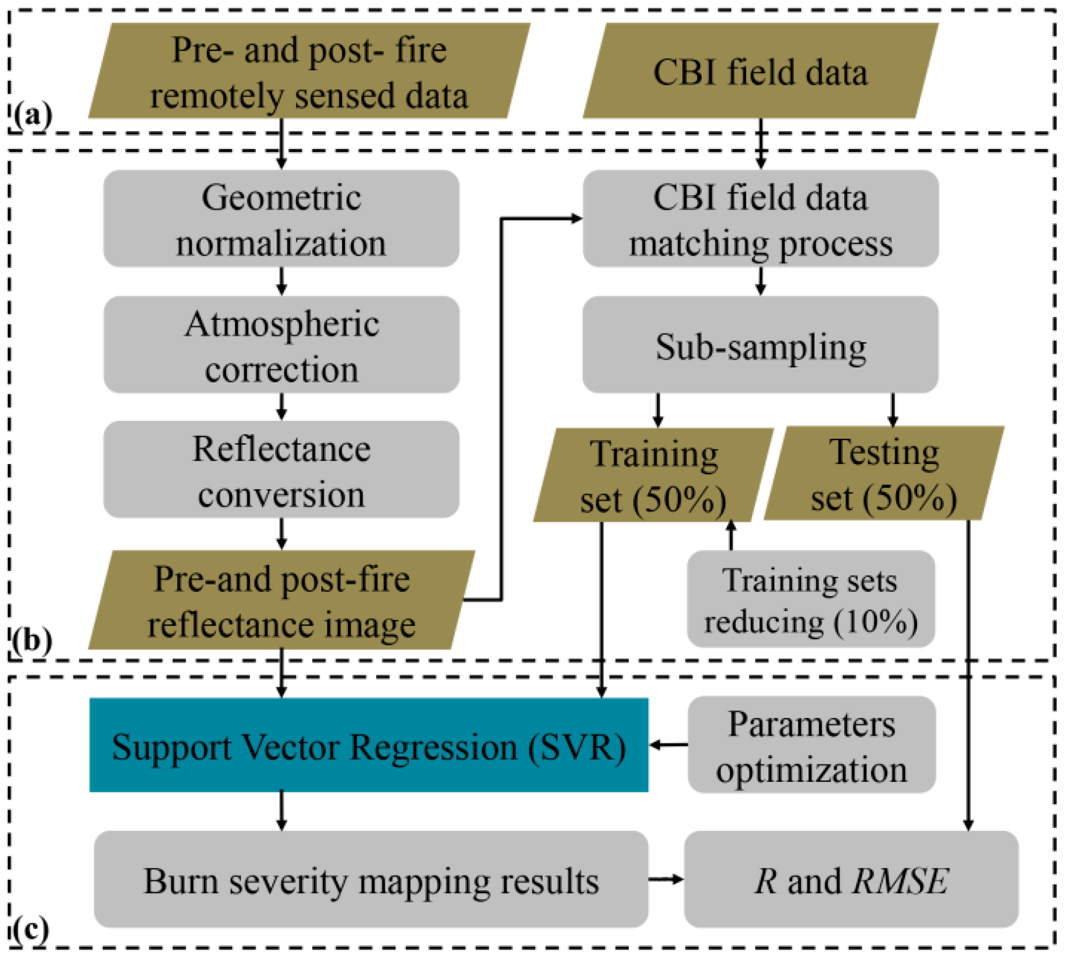
The TM/ETM+ images have already been recognized as the most suitable remotely sensed data for burn severity mapping [4,11]. Therefore, multi-temporal TM/ETM+ images were collected in five forest fires (

Table 1. Summary of characteristics of forest fires and datasets used in this study.

Fire Name	Bear	Jasper	Mule	Pw03-Wolf
Regional Eco-Types	Southwest	Central	Northern Rockies	California
Alarm Date	27 June 2002	24 August 2000	11 July 2002	3 Octorber 2002–11 July 2002
Sensor	TM	TM and ETM+	TM	ETM+ and TM
Pre-fire Image Date	13 June 2002	1 May 2000	21 September 2001	18 Octorber 2001
Post-fire Image Date	31 May 2003	31 May 2002	27 September 2003	16 Octorber 2003
Landsat Path/Row	36/32	33/30	37/30	42/34
CBI Field Plots Collected Date	28 May–30 May 2003	14 May–26 May 2002	8 September–11 September 2003	15 August–30 Octorber 2003
Fire Size (km2)	18.62	336.37	11.86	13.61

). For each fire, we obtained the post-fire image acquired around the time when the field data was collected, which can minimize the plant phenology differences between the image acquisition and the field data collection. Pre-fire TM or ETM+ images acquired at the same season one or two years before the acquisition of post-fire image were also obtained for each fire. This was helpful for reducing the differences in sun angle, atmospheric effects and plant phenology [28], when the multi-temporal images were used in this study. All of these images with the Level L1G of processing were downloaded from the U.S. Geological Survey EarthExplorer (USGS 2013). Their pre-processing, including atmospheric correction, geometric normalization and reflectance conversion, was conducted using ENVI 5.0 software (ITT Visual Information Solutions, Boulder, CO, USA).

According to the coordinates recorded by GPS in the field, the field-measurement data points were matched with the corresponding pixel in the remote sensing image. The spectral reflectance of remote sensing images was then extracted by using a 3 × 3 pixel matrix to reduce the effect of the GPS positioning error [6,53]. This matching process was realized using ArcGIS 9.3 software (EsriChina, Beijing, China).

3. Methods

3.1. Support Vector Regression

The basic learning problems addressed by traditional/statistical regression are to establish an unknown model $f\left(w,x\right)$ (i.e., the quantitative relationship between input and output), based on a limited number of training samples: $\left(x_1,y_1\right),\left(x_2,y_2\right),\cdots ,\left(x_n,y_n\right)$ [43,54,55], as in Equation (1).

$$f\left(w,x\right)={\displaystyle \sum _{i=1}^n{w}_i{g}_i\left(x\right)}+b$$

(1)

where $w_i$ means a set of parameters in regression function, $g_i\left(x\right)$ represents a set of non-linear transformations, and b denotes the “bias” term.

Traditionally, when estimating model parameters, we only consider the prediction risk. This can ensure that the model has a better performance on limited training samples [43]. Most typical prediction risk measures are based on the Empirical Risk Minimization (ERM) [54,55], which can be determined by Equation (2).

$$R\left(w\right)=R{\left(w\right)}_{ERM}={\displaystyle \int L\left(y,f\left(w,x\right)\right)}p\left(x,y\right)dxdy$$

(2)

where $L\left(y,f\left(w,x\right)\right)$ is the loss function, and the training sample is assumed to satisfy some (unknown) distributions, which can be defined as a joint probability density function $p\left(x,y\right)$.

However, in actual applications, both excellent performance on training samples and good generalization on unknown samples (i.e., predicting samples) are needed from the model. Therefore, the Structural Risk Minimization (SRM), an inductive principle based on the Vapnik-Chervonenkis theory (VC-theory, a form of computational learning theory), has been introduced in the SVR modeling [54,55]. Based on the VC-theory, the model generalization is affected by the complexity of model and the number of training samples, as expressed in Equation (3).

$$R\left(w\right)\le R{\left(w\right)}_{ERM}+H(h/n)$$

(3)

where $H(•)$ is often called trust scope, h means a measure of model complexity (VC-dimension), and n represents the number of training samples.

Therefore, according to the above SRM principle, the model generalization of support vector regression (SVR) can be improved by reducing the model complexity and selecting the training samples. Specifically, the SVR model estimation procedure can be expressed as a convex optimization problem solving [43,44,54,55,56]:

$$\begin{array}{ll}\mathrm{minimize}& \frac{1}{2}{\Vert w\Vert }^2+C{\displaystyle \sum _{i=1}^n\left({\xi }_i+{\xi }_i^{\ast }\right)}\\ \mathrm{subject}\mathrm{to}& \{\begin{array}{c}{y}_i-f\left(x_i,w\right)-b\le \epsilon +{\xi }_i^{\ast }\\ f\left(x_i,w\right)+b-y_i\le \epsilon +{\xi }_i\\ {\xi }_i,{\xi }_i^{\ast }\ge 0\end{array}\end{array}$$

(4)

where the ${\Vert w\Vert }^2$ measures the model complexity and the constant $C>0$ determines the tradeoff between the smoothness of model and the amount up to which the deviations larger than $\epsilon$ are tolerated [54]. Slack variables (${\xi }_i$, ${\xi }_i^{\ast }$), which are used to measure the deviation of training samples outside ε-insensitive zone, are based on a different type of loss function (ε-insensitive loss function) proposed by Vapnik for SVR [43,54,55]:

$${\left|\xi \right|}_{\epsilon }=L\left(y,f\left(x,w\right)\right)=\{\begin{array}{cc}\left|y-f\left(x,w\right)\right|-\epsilon & \mathrm{otherwise}\hfill \\ 0& \mathrm{if}\left|y-f\left(x,w\right)\right|\le \epsilon \hfill \end{array}$$

(5)

By introducing Lagrange multipliers (${\alpha }_i$, ${\alpha }_i^{\ast }$) and kernel function $K\left(x_i,x\right)$, this convex optimization problem can be then transformed into a dual problem based on the Wolfe duality theory [43,44,54,55]:

$$\max W\left(\alpha \right)=-\frac{1}{2}{\displaystyle \sum _{i,j=1}^n\left({\alpha }_i-{\alpha }_i^{\ast }\right)\left({\alpha }_j-{\alpha }_j^{\ast }\right)}K\left(x_i,x_j\right)-\epsilon {\displaystyle \sum _{i=1}^n\left({\alpha }_i+{\alpha }_i^{\ast }\right)}+{\displaystyle \sum _{i=1}^n{y}_i\left({\alpha }_i-{\alpha }_i^{\ast }\right)}$$

(6)

$$\mathrm{subject}\mathrm{to}\{\begin{array}{l}{\displaystyle \sum _{i=1}^n\left({\alpha }_i-{\alpha }_i^{\ast }\right)=0}\\ {\alpha }_i,{\alpha }_i^{\ast }\in \left[0,C\right]\end{array}$$

(7)

The established SVR model can be expressed as follows [43,44,54,55,56]:

$$f\left(x\right)={\displaystyle \sum _{i=1}^n\left({\alpha }_i-{\alpha }_i^{\ast }\right)}K\left(x_i,x\right)+b$$

(8)

where Lagrange multipliers (${\alpha }_i$, ${\alpha }_i^{\ast }$) for every training sample cannot be nonzero at the same time. Consequently, those training samples are named support vectors (SVs).

3.2. SVR Modeling

The software platform for the SVR modeling in this study was the LIBSVM Toolbox of Matlab 2011b which can be downloaded on website (https://www.csie.ntu.edu.tw/~cjlin/libsvm/index.html) [57]. The hardware platform was a Personal Computer with CPU 1333 MHz and 2 GB RAM.

Similar to traditional/statistical regression methods, the parameters optimization for the SVR modeling also was needed, since appropriate setting of the key parameters (i.e., kernel parameters, C, and ε) can basically affect the SVR performance [54,58]. The procedures for parameter optimization are described in the following.

3.2.1. Kernel Parameters

Kernel parameters (i.e., kernel type and kernel function parameters) are related to the distribution of the input values of the training set and their selections are usually based on application-domain knowledge [54]. For regression tasks in this study, based on several trials, it has been found that both the linear kernel and the RBF kernel selecting can ensure that the SVR exhibits good performance. Although the RBF kernel is more widely used in remote sensing applications, we selected linear kernel as optimal Kernel Parameters in this study, since this selection can keep us only focus on the choice of C and ε [54]. The following optimization procedures can be simplified.

3.2.2. Regularization Parameter

Regularization parameter C > 0 determines the tradeoff between the complexity of model (${\Vert w\Vert }^2$) and the amount up to which the deviations larger than ε are tolerated. Larger C makes the objective of optimization formulation intend to focus more on minimizing the empirical risk [54]. On the other hand, if C is too small, sufficient stress will be placed on minimizing the model complexity.

3.2.3. Parameter ε

Parameter ε controls the width of the ε-insensitive zone used to select the number of support vectors. Bigger ε means that more training samples inside ε-insensitive zone will be eliminated, which can result in “flatter” (i.e., less complex) estimates [54]. Hence, in this study, the ability of SVR model generalization was affected by C and ε.

Generally, these two parameters are determined by the above parameter optimization process. They can be defined based on the grid search method [38,57]. This search method includes the following three steps:

• Different types of parameters are paired together within the assigned ranges of these parameters.
• With a selected pair of parameters in a search grid, the SVR are trained and then the common three-fold cross-validation precision (i.e., the root mean squared error (RMSE) between the predicted and the observed CBI values) is obtained and recorded.
• By altering the parameters pairs in other search grids, a series of cross-validation RMSEs are then returned too. Finally, the pair of key parameters of SVR (C and ε) with the minimum cross-validation RMSE value is selected.

3.3. Performance Evaluations

To evaluate the performance of SVR-based mapping methods, its predicted CBI values with the observed CBI values of testing field data were compared. The Correlation Coefficient (R) and the RMSE (recommended by DeSantisandChuvieco [8]) for the testing set were calculated. Further, these performance measurements of the SVR-based mapping method were evaluated by comparing to those of the RA method. Specifically, the model for the RA method was dNBR-based quadratic nonlinear regression [46,59,60]. The calculations of R and RMSE are shown as follows.

$$R=\frac{{\displaystyle \sum _{i=1}^n\left(CB{I}_i^{\mathrm{predicted}}-\overline{CB{I}^{\mathrm{predicted}}}\right)\left(CB{I}_i^{\mathrm{observed}}-\overline{CB{I}^{\mathrm{observed}}}\right)}}{\sqrt{{\displaystyle \sum _{i=1}^n{\left(CB{I}_i^{\mathrm{predicted}}-\overline{CB{I}^{\mathrm{predicted}}}\right)}^2}{\displaystyle \sum _{i=1}^n{\left(CB{I}_i^{\mathrm{observed}}-\overline{CB{I}^{\mathrm{observed}}}\right)}^2}}}$$

(9)

$$RMSE=\sqrt{\frac{{\displaystyle \sum _{i=1}^n{\left(CB{I}_i^{\mathrm{predicted}}-CB{I}_i^{\mathrm{observed}}\right)}^2}}{n}}$$

(10)

Moreover, an additional experiment (see Figure 2) was designed in this study to test the capabilities of the SVR-based mapping method in handling limited number of field samples, in which the number of training samples for each fire was randomly reduced by the 10%.

4. Results and Discussion

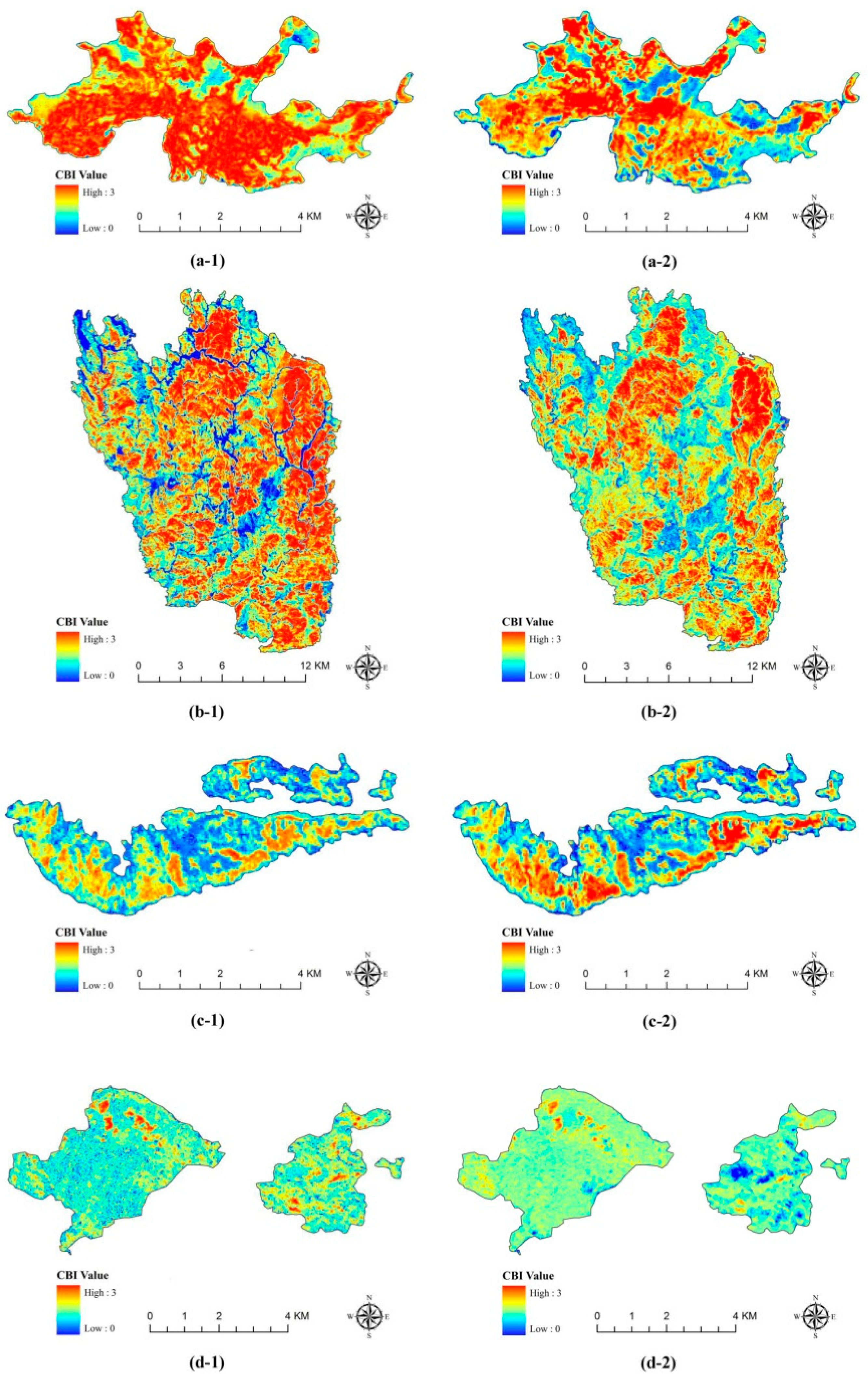
4.1. SVR-Based Burn Severity Mapping and Performance Evaluation

Figure 3 shows the SVR-based burn severity mapping results. The burn severity is also mapped using RA methods (based on dNBR) in Figure 3. From a visual perspective, the spatial distributions of burn severity are more detailed in SVR-based maps than that of RA-based maps. The correlation coefficient (R) and root mean squared error (RMSE) between the predicted and the observed CBI values of the testing set are presented in

Table 2. Summary of parameters and precisions of RA- and SVR-based methods.

Fire Name	RA Parameters				RA 1 Precisions		SVR Parameters		SVR Precisions
	a	b	c	R2	R	RMSE	C	ε	R	RMSE
Bear Fire	−15.22	9.53	1.35	0.52	0.82	0.60	16	0.22	0.85	0.54
Jasper Fire	−4.39	5.77	0.82	0.68	0.73	0.68	29.86	0.03	0.83	0.57
Mule Fire	−0.63	3.58	0.51	0.60	0.85	0.53	4	0.23	0.87	0.50
Pw03-wolf Fire	−3.75	5.55	0.68	0.61	0.78	0.53	11.31	0.25	0.89	0.46

¹ The model for RA method is CBI^predicted = a × (dNBR)² + b × (dNBR) + c (all p values < 0.05).

. The R value for SVR-based method is between 0.83 and 0.89, which is larger than that of RA method (R: 0.73–0.85). The RMSE value of SVR-based method (0.46–0.57) is smaller than that of RA method (0.53–0.68) (see Table 2).

The above results indicate that the SVR-based method performed better than RA method. According to statistics of the TM band reflectance response to burn severity [4], the obvious changes of each TM band reflectance between pre- and post-fire remote sensing images can be observed. This indicates that each TM band might contain specific information about burn severity. The SVR-based burn severity mapping fully uses the spectral information contained in all bands of remote sensing images, while most spectral indices of burn severity in previous studies use only two spectral bands of remote sensing images, for example, the dNBR calculation for RA method only uses near-infrared spectral band (RNIR) and shortwave-infrared spectral band (RSWIR_2.2) in multi-temporal images. Therefore, the full use of spectral information contained in the remotely sensed data makes the SVR-based method to reveal spatial distributions of burn severity in more details.

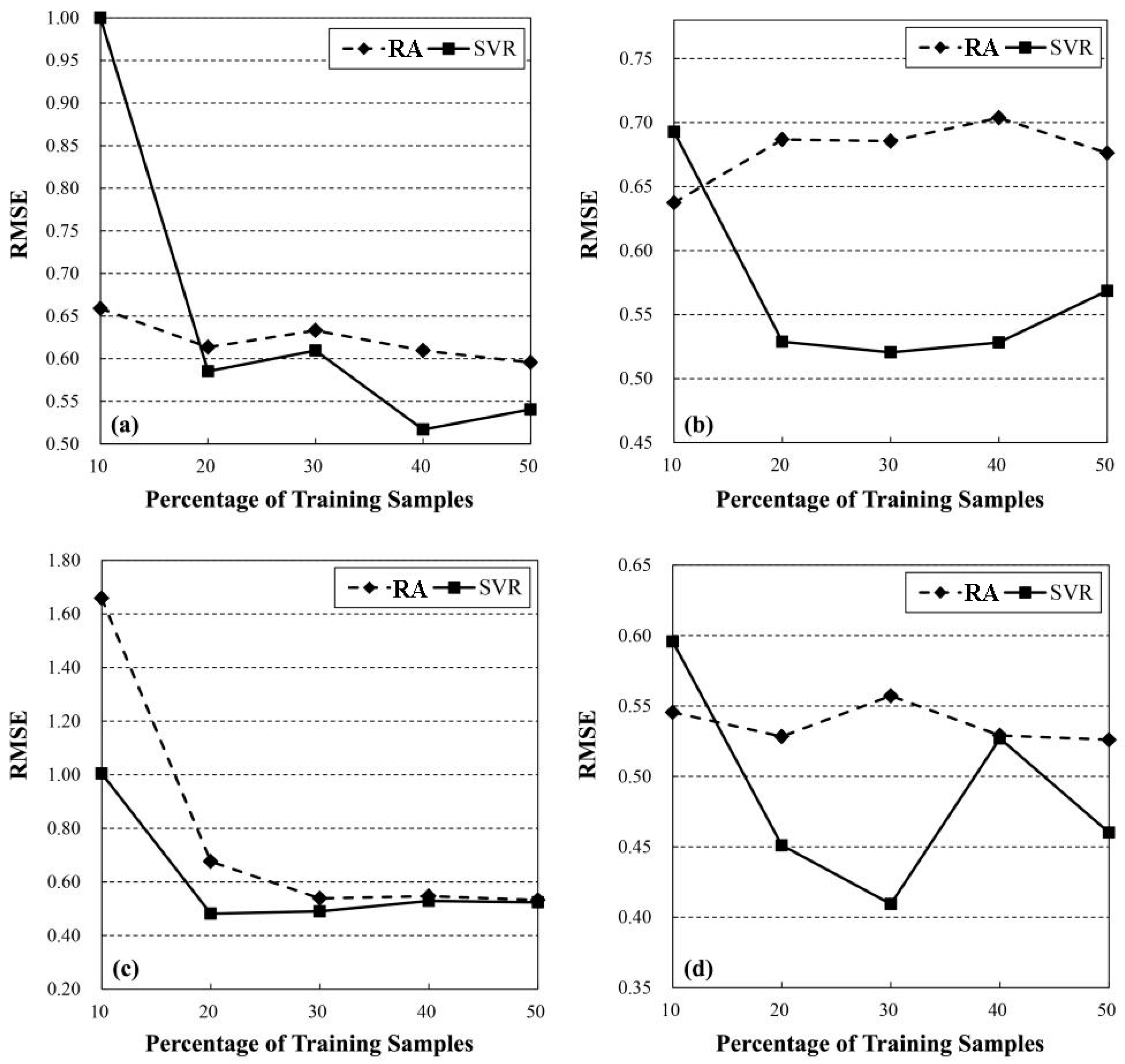
4.2. Burn Severity Mapping Accuracy Sensitivity to Training Samples

Figure 4 shows the generalization performances of both SVR-based and RA methods in the case of small sample size. We find that the accuracy of both methods varies with the reduction of training samples (by 10%). In particular, the overall precision measured by RMSE indicates that SVR outperformed RA during the reduction of training samples size (more details about training samples can be found in

Table 3. Summary of precisions of RA- and SVR-based methods during the reduction of training samples size.

Fire Name	Field Plots Number		RA Precisions		SVR Precisions
	Training Samples	Testing Samples	R	RMSE	R	RMSE
Bear Fire	6	49	0.81	0.66	0.71	1.00
	11	44	0.81	0.61	0.86	0.59
	17	38	0.80	0.63	0.80	0.61
	22	33	0.82	0.61	0.87	0.52
	28	27	0.82	0.60	0.85	0.54
Jasper Fire	8	68	0.73	0.64	0.64	0.69
	15	61	0.73	0.69	0.82	0.53
	23	53	0.72	0.69	0.83	0.52
	30	46	0.72	0.70	0.83	0.53
	38	38	0.73	0.68	0.83	0.57
Mule Fire	6	49	−0.19	1.66	0.00	1.00
	11	44	0.83	0.68	0.89	0.48
	17	38	0.86	0.54	0.88	0.49
	22	33	0.86	0.55	0.87	0.53
	28	27	0.85	0.53	0.87	0.50
Pw03-wolf Fire	8	70	0.78	0.55	0.77	0.60
	16	62	0.78	0.53	0.84	0.45
	23	55	0.77	0.56	0.87	0.41
	31	47	0.78	0.53	0.87	0.53
	39	39	0.78	0.53	0.89	0.46

). This fact is supported by that of previous studies of other fields [35,36].

It is believed that the better performance of SVR on small number of field plots should attribute to its better model generalization in case of limited training samples. As described in Section 2.1, a measurement of model complexity (i.e., ${\Vert w\Vert }^2$) has been introduced into the objective function of the SVR model. It can be reduced by adjusting a specific parameter (i.e., ε). With a bigger ε, more training samples inside ε-insensitive zone will be eliminated, which can result in “less complex” estimates (i.e., better generalization) [54]. This means that only those remaining training samples (i.e., named support vectors) can actually affect the mapping results. If these non-support vectors are eliminated in the training process, the SVR generalization performance will not be affected, which means that the SVR is less sensitive to the reduction of training samples size.

In Figure 4 and Table 3, it can be seen that the SVR performed poorly, when 10% training sets were selected to train it. This could be explained by the fact that the number of training sets is too small (i.e., training field plots number is 6–8). With very few training samples, the Empirical Risk Minimization (ERM) of SVR-based method will be enlarged extremely. Although its effect on model generalization can be adjusted by parameter C, this kind of adjustment will not sufficiently improve the model generalization in this situation. This has reconfirmed an appropriate balance (i.e., C) between the complexity of the model and the ERM is needed during the parameter optimization process of SVR.

Based on above discussion, we can conclude that the SVR can map the burn severity accurately and achieve relatively better generalization performance even with fewer training sets. This method should be recommended in future research.

5. Conclusions

In this study, the SVR-based burn severity mapping method was proposed to accurately obtain the burn severity of forest fires using multi-temporal images. The evaluation of this method was carried out by comparing the predicted and observed CBI values of training sets, and compared with the dNBR-based RA method. The results demonstrated that the performance of the SVR-based mapping method is more accurate than that of the RA method. Even with a smaller number of training sets, it can map the detailed distribution of burn severity of forest fires and achieve relatively better generalization, compared to RA burn severity mapping methods. Therefore, the SVR-based mapping method with better generalization performance should be recommended in future research of burn severity of forest fires.

References

1. Quintano, C.; Fernández-Manso, A.; Roberts, D.A. Multiple endmember spectral mixture analysis (mesma) to map burn severity levels from landsat images in mediterranean countries. Remote Sens. Environ. 2013, 136, 76–88. [Google Scholar] [CrossRef]
2. Veraverbeke, S.; Hook, S.; Hulley, G. An alternative spectral index for rapid fire severity assessments. Remote Sens. Environ. 2012, 123, 72–80. [Google Scholar] [CrossRef]
3. Zheng, Z.; Huang, W.; Li, S.; Zeng, Y. Forest fire spread simulating model using cellular automaton with extreme learning machine. Ecol. Model. 2017, 348, 33–43. [Google Scholar] [CrossRef]
4. Key, C.H.; Benson, N.C. Landscape Assessment (la): Sampling and Analysis Methods; Rocky Mountain Research Station, USDA, Forest Service: Fort Collins, CO, USA, 2006; pp. LA-1–LA-51.
5. Veraverbeke, S.; Verstraeten, W.W.; Lhermitte, S.; Van De Kerchove, R.; Goossens, R. Assessment of post-fire changes in land surface temperature and surface albedo, and their relation with fire-burn severity using multitemporal modis imagery. Int. J. Wildl. Fire 2012, 21, 243–256. [Google Scholar] [CrossRef]
6. Zheng, Z.; Zeng, Y.; Li, S.; Huang, W. A new burn severity index based on land surface temperature and enhanced vegetation index. Int. J. Appl. Earth Obs. Geoinf. 2016, 45, 84–94. [Google Scholar] [CrossRef]
7. Key, C.; Benson, N. Landscape assessment: Ground measure of severity, the composite burn index; and remote sensing of severity, the normalized burn ratio. In FIREMON: Fire Effects Monitoring and Inventory System; Lutes, D.C., Keane, R.E., Caratti, J.F., Key, C.H., Benson, N.C., Gangi, L.J., Eds.; USDA Forest Service, Rocky Mountain Research Station: Fort Collins, CO, USA, 2006; pp. CD:LA1–CD:LA51. [Google Scholar]
8. De Santis, A.; Chuvieco, E. Geocbi: A modified version of the composite burn index for the initial assessment of the short-term burn severity from remotely sensed data. Remote Sens. Environ. 2009, 113, 554–562. [Google Scholar] [CrossRef]
9. Schepers, L.; Haest, B.; Veraverbeke, S.; Spanhove, T.; Vanden Borre, J.; Goossens, R. Burned area detection and burn severity assessment of a heathland fire in belgium using airborne imaging spectroscopy (apex). Remote Sens. 2014, 6, 1803–1826. [Google Scholar] [CrossRef]
10. Montealegre, A.; Lamelas, M.; Tanase, M.; De la Riva, J. Forest fire severity assessment using als data in a mediterranean environment. Remote Sens. 2014, 6, 4240–4265. [Google Scholar] [CrossRef]
11. Parks, S.; Dillon, G.; Miller, C. A new metric for quantifying burn severity: The relativized burn ratio. Remote Sens. 2014, 6, 1827–1844. [Google Scholar] [CrossRef]
12. Kasischke, E.S.; French, N.H. Locating and estimating the areal extent of wildfires in alaskan boreal forests using multiple-season avhrr ndvi composite data. Remote Sens. Environ. 1995, 51, 263–275. [Google Scholar] [CrossRef]
13. Remmel, T.K.; Perera, A.H. Fire mapping in a northern boreal forest: Assessing avhrr/ndvi methods of change detection. For. Ecol. Manag. 2001, 152, 119–129. [Google Scholar] [CrossRef]
14. Edwards, A.C.; Maier, S.W.; Hutley, L.B.; Williams, R.J.; Russell-Smith, J. Spectral analysis of fire severity in north australian tropical savannas. Remote Sens. Environ. 2013, 136, 56–65. [Google Scholar] [CrossRef]
15. George, C.; Rowland, C.; Gerard, F.; Balzter, H. Retrospective mapping of burnt areas in central siberia using a modification of the normalised difference water index. Remote Sens. Environ. 2006, 104, 346–359. [Google Scholar] [CrossRef]
16. Gerard, F.; Plummer, S.; Wadsworth, R.; Ferreruela Sanfeliu, A.; Iliffe, L.; Balzter, H.; Wyatt, B. Forest fire scar detection in the boreal forest with multitemporal spot-vegetation data. IEEE Trans. Geosci. Remote Sens. 2003, 41, 2575–2585. [Google Scholar] [CrossRef] [Green Version]
17. Loboda, T.V.; French, N.H.F.; Hight-Harf, C.; Jenkins, L.; Miller, M.E. Mapping fire extent and burn severity in alaskan tussock tundra: An analysis of the spectral response of tundra vegetation to wildland fire. Remote Sens. Environ. 2013, 134, 194–209. [Google Scholar] [CrossRef]
18. Murphy, K.A.; Reynolds, J.H.; Koltun, J.M. Evaluating the ability of the differenced normalized burn ratio (dnbr) to predict ecologically significant burn severity in alaskan boreal forests. Int. J. Wildl. Fire 2008, 17, 490–499. [Google Scholar] [CrossRef]
19. Wang, L.; Qu, J.J.; Hao, X. Forest fire detection using the normalized multi-band drought index (nmdi) with satellite measurements. Agric. For. Meteorol. 2008, 148, 1767–1776. [Google Scholar] [CrossRef]
20. Weber, K.T.; Seefeldt, S.S.; Norton, J.M.; Finley, C. Fire severity modeling of sagebrush-steppe rangelands in southeastern Idaho. GISci. Remote Sens. 2008, 45, 68–82. [Google Scholar] [CrossRef]
21. Cocke, A.E.; Fulé, P.Z.; Crouse, J.E. Comparison of burn severity assessments using differenced normalized burn ratio and ground data. Int. J. Wildl. Fire 2005, 14, 189–198. [Google Scholar] [CrossRef]
22. Epting, J.; Verbyla, D.; Sorbel, B. Evaluation of remotely sensed indices for assessing burn severity in interior Alaska using Landsat tm and ETM+. Remote Sens. Environ. 2005, 96, 328–339. [Google Scholar] [CrossRef]
23. Escuin, S.; Navarro, R.; Fernandez, P. Fire severity assessment by using NBR (normalized burn ratio) and NDVI (normalized difference vegetation index) derived from Landsat tm/ETM images. Int. J. Remote Sens. 2008, 29, 1053–1073. [Google Scholar] [CrossRef]
24. Garcia, M.L.; Caselles, V. Mapping burns and natural reforestation using thematic mapper data. Geocarto Int. 1991, 6, 31–37. [Google Scholar] [CrossRef]
25. Key, C.H.; Benson, N.C. The Normalized Burn Ratio (NBR): A Landsat tm Radiometric Measure of Burn Severity. Available online: http://www.nrmsc.usgs.gov/research/ndbr.htm (accessed on 22 January 2012).
26. Van Wagtendonk, J.W.; Root, R.R.; Key, C.H. Comparison of aviris and Landsat ETM+ detection capabilities for burn severity. Remote Sens. Environ. 2004, 92, 397–408. [Google Scholar] [CrossRef]
27. Miller, J.D.; Thode, A.E. Quantifying burn severity in a heterogeneous landscape with a relative version of the delta normalized burn ratio (DNBR). Remote Sens. Environ. 2007, 109, 66–80. [Google Scholar] [CrossRef]
28. De Santis, A.; Chuvieco, E. Burn severity estimation from remotely sensed data: Performance of simulation versus empirical models. Remote Sens. Environ. 2007, 108, 422–435. [Google Scholar] [CrossRef]
29. Hudak, A.T.; Morgan, P.; Bobbitt, M.J.; Smith, A.M.S.; Lewis, S.A.; Lentile, L.B.; Robichaud, P.R.; Clark, J.T.; McKinley, R.A. The relationship of multispectral satellite imagery to immediate fire effects. Fire Ecol. 2007, 3, 64–90. [Google Scholar] [CrossRef]
30. Roy, D.P.; Boschetti, L.; Trigg, S.N. Remote sensing of fire severity: Assessing the performance of the normalized burn ratio. IEEE Geosci. Remote Sens. Lett. 2006, 3, 112–116. [Google Scholar] [CrossRef]
31. Wulder, M.A.; White, J.C.; Alvarez, F.; Han, T.; Rogan, J.; Hawkes, B. Characterizing boreal forest wildfire with multi-temporal Landsat and Lidar data. Remote Sens. Environ. 2009, 113, 1540–1555. [Google Scholar] [CrossRef]
32. Patterson, M.W.; Yool, S.R. Mapping fire-induced vegetation mortality using landsat thematic mapper data: A comparison of linear transformation techniques. Remote Sens. Environ. 1998, 65, 132–142. [Google Scholar] [CrossRef]
33. Brewer, C.K.; Winne, J.C.; Redmond, R.L.; Opitz, D.W.; Mangrich, M.V. Classifying and mapping wildfire severity: A comparison of methods. Photogramm. Eng. Remote Sens. 2005, 71, 1311–1320. [Google Scholar] [CrossRef]
34. Quintano, C.; Fernandez-Manso, A.; Roberts, D.A. Burn severity mapping from landsat mesma fraction images and land surface temperature. Remote Sens. Environ. 2017, 190, 83–95. [Google Scholar] [CrossRef]
35. Camps-Valls, G.; Bruzzone, L.; Rojo-Álvarez, J.L.; Melgani, F. Robust support vector regression for biophysical variable estimation from remotely sensed images. IEEE Geosci. Remote Sens. Lett. 2006, 3, 339–343. [Google Scholar] [CrossRef]
36. Shao, Y.; Lunetta, R.S. Comparison of support vector machine, neural network, and cart algorithms for the land-cover classification using limited training data points. ISPRS-J. Photogramm. Remote Sens. 2012, 70, 78–87. [Google Scholar] [CrossRef]
37. Hollander, M.; Wolfe, D.A.; Chicken, E. Nonparametric Statistical Methods; John Wiley & Sons: New York, NY, USA, 2013. [Google Scholar]
38. Sadri, S.; Burn, D.H. Nonparametric methods for drought severity estimation at ungauged sites. Water Resour. Res. 2012, 48, W12505. [Google Scholar] [CrossRef]
39. Huang, C.; Davis, L.S.; Townshend, J.R.G. An assessment of support vector machines for land cover classification. Int. J. Remote Sens. 2002, 23, 725–749. [Google Scholar] [CrossRef]
40. Belayneh, A.; Adamowski, J. Standard precipitation index drought forecasting using neural networks, wavelet neural networks, and support vector regression. Appl. Comput. Intell. Soft Comput. 2012, 2012, 1–13. [Google Scholar] [CrossRef]
41. Osowski, S.; Garanty, K. Forecasting of the daily meteorological pollution using wavelets and support vector machine. Eng. Appl. Artif. Intell. 2007, 20, 745–755. [Google Scholar] [CrossRef]
42. Hultquist, C.; Chen, G.; Zhao, K. A comparison of gaussian process regression, random forests and support vector regression for burn severity assessment in diseased forests. Remote Sens. Lett. 2014, 5, 723–732. [Google Scholar] [CrossRef]
43. Vapnik, V.N. Statistical Learning Theory; Wiley: New York, NY, USA, 1998. [Google Scholar]
44. Vapnik, V.N. The Nature of Statistical Learning Theory; Springer: New York, NY, USA, 2000. [Google Scholar]
45. Perryman, B.L.; Olson, R.A.; Petersburg, S.; Naumann, T. Vegetation response to prescribed fire in Dinosaur National Monument. West. N. Am. Nat. 2002, 62, 414–422. [Google Scholar]
46. Chen, X.; Vogelmann, J.E.; Rollins, M.; Ohlen, D.; Key, C.H.; Yang, L.; Huang, C.; Shi, H. Detecting post-fire burn severity and vegetation recovery using multitemporal remote sensing spectral indices and field-collected composite burn index data in a ponderosa pine forest. Int. J. Remote Sens. 2011, 32, 7905–7927. [Google Scholar] [CrossRef]
47. Brown, P.M.; Sieg, C.H. Historical variability in fire at the ponderosa pine-Northern Great Plains prairie ecotone, southeastern Black Hills, South Dakota. Ecoscience 1999, 6, 539–547. [Google Scholar] [CrossRef]
48. Smith, A.M.S.; Lentile, L.B.; Hudak, A.T.; Morgan, P. Evaluation of linear spectral unmixing and ΔNBR for predicting post-fire recovery in a North American ponderosa pine forest. Int. J. Remote Sens. 2007, 28, 5159–5166. [Google Scholar] [CrossRef]
49. Berg, N.D.; Gese, E.M.; Squires, J.R.; Aubry, L.M. Influence of forest structure on the abundance of snowshoe hares in western Wyoming. J. Wildl. Manag. 2012, 76, 1480–1488. [Google Scholar] [CrossRef] [Green Version]
50. Guarín, A.; Taylor, A.H. Drought triggered tree mortality in mixed conifer forests in Yosemite National Park, California, USA. For. Ecol. Manag. 2005, 218, 229–244. [Google Scholar] [CrossRef]
51. Zhu, Z.; Key, C.; Ohlen, D.; Benson, N.C. Evaluate Sensitivities of Burn-Severity Mapping Algorithms for Different Ecosystems and Fire Histories in the United States; Final Report to the Joint Fire Science Program; Project: JFSP 01-1-4-12; USGS EROS: Sioux Falls, SD, USA, 2006.
52. Shamshirband, S.; Gocic, M.; Petkovic, D.; Saboohi, H.; Herawan, T.; Mat Kiah, L.; Akib, S. Soft-Computing Methodologies for Precipitation Estimation: A Case Study. IEEE J. Sel. Top. Appl. Earth Obs. Remote Sens. 2015, 8, 1353–1358. [Google Scholar] [CrossRef]
53. Chuvieco, E.; Cocero, D.; Riano, D.; Martin, P.; Martınez-Vega, J.; de la Riva, J.; Pérez, F. Combining NDVI and surface temperature for the estimation of live fuel moisture content in forest fire danger rating. Remote Sens. Environ. 2004, 92, 322–331. [Google Scholar] [CrossRef] [Green Version]
54. Cherkassky, V.; Ma, Y. Practical selection of SVM parameters and noise estimation for SVM regression. Neural Netw. 2004, 17, 113–126. [Google Scholar] [CrossRef] [Green Version]
55. Vapnik, V.N. An overview of statistical learning theory. IEEE Trans. Neural Netw. 1999, 10, 988–999. [Google Scholar] [CrossRef] [PubMed]
56. Zhang, X. Introduction to statistical learning theory and support vector machines. Acta Autom. Sin. 2000, 26, 32–42. [Google Scholar]
57. Chang, C.-C.; Lin, C.-J. LIBSVM: A library for support vector machines. ACM Trans. Intell. Syst. Technol. 2011, 2, 27. [Google Scholar] [CrossRef]
58. Mas, J.F.; Flores, J.J. The application of artificial neural networks to the analysis of remotely sensed data. Int. J. Remote Sens. 2008, 29, 617–663. [Google Scholar] [CrossRef]
59. De Santis, A.; Asner, G.P.; Vaughan, P.J.; Knapp, D.E. Mapping burn severity and burning efficiency in California using simulation models and Landsat imagery. Remote Sens. Environ. 2010, 114, 1535–1545. [Google Scholar] [CrossRef]
60. Soverel, N.O.; Perrakis, D.D.B.; Coops, N.C. Estimating burn severity from Landsat dNBR and RdNBR indices across western Canada. Remote Sens. Environ. 2010, 114, 1896–1909. [Google Scholar] [CrossRef]
Figure 1. Study area locations (Landsat TM/ETM+ image, R: R7, G: R4, B: R1). ① is Bear Fire, ② is Jasper Fire, ③ is Mule Fire, and ④ are Pw03 Fire and Wolf Fire.
Forests 09 00608 g001
Figure 2. The flowchart of SVR overall process. (a) Is data collection, (b) are data pre-processing and SVR modeling, and (c) is performance evaluations.
Forests 09 00608 g002
Figure 3. Burn severity maps, expressed as Composite Burn Index (CBI) and calculated by using the RA (based on dNBR) and the SVR in five fires: (a-1) the RA mapping results of the Bear Fire; (a-2) the SVR mapping results of the Bear Fire; (b-1) the RA mapping results of the Jasper Fire; (b-2) the SVR mapping results of the Jasper Fire; (c-1) the RA mapping results of the Mule Fire; (c-2) the SVR mapping results of the Mule Fire; (d-1) the RA mapping results of the Pw03-wolf Fires; and (d-2) the SVR mapping results of the Pw03-Wolf Fires.
Forests 09 00608 g003
Figure 4. Comparison of overall performance for the SVR- and RA-based methods using different percentages of training samples: (a) Bear Fire; (b) Jasper Fire; (c) Mule Fire; and (d) Pw03-wolf Fire. RMSE represents the Root Mean Square Error.
Forests 09 00608 g004