A Comparison of Simulated and Field-Derived Leaf Area Index (LAI) and Canopy Height Values from Four Forest Complexes in the Southeastern USA

Abstract
1. Introduction
2. Materials and Methods
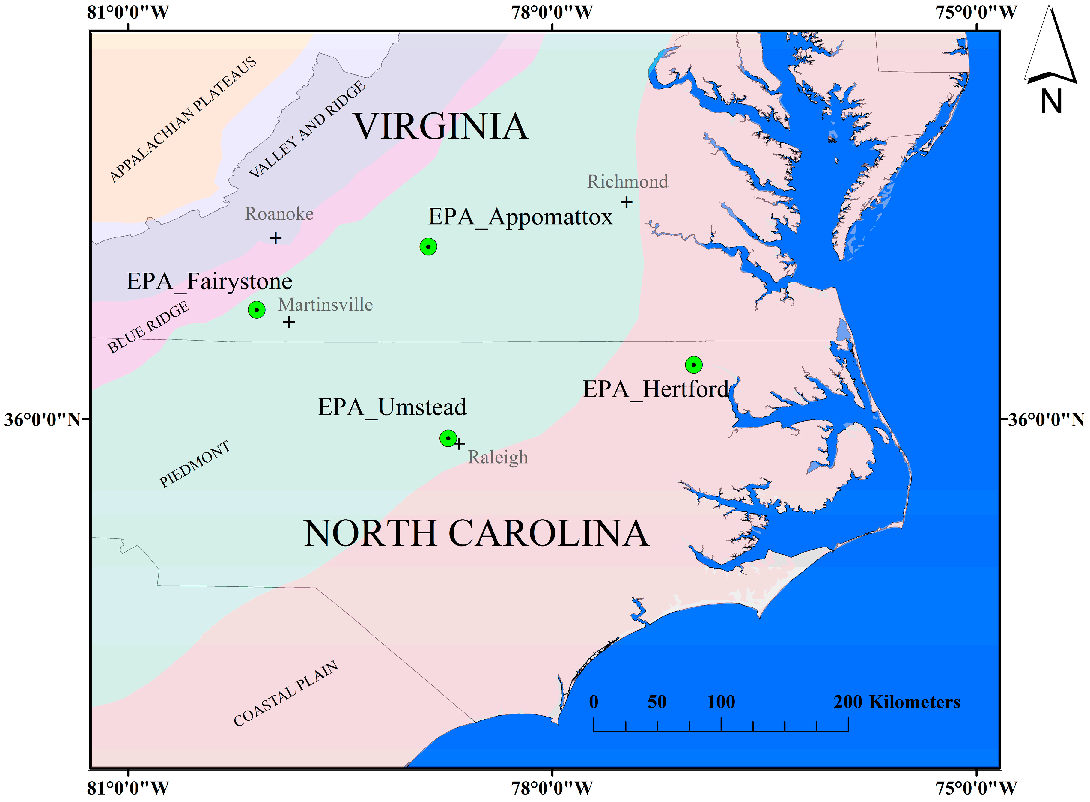
2.1. Site Descriptions
2.1.1. Appomattox
2.1.2. Hertford
2.1.3. Fairystone
2.1.4. Umstead
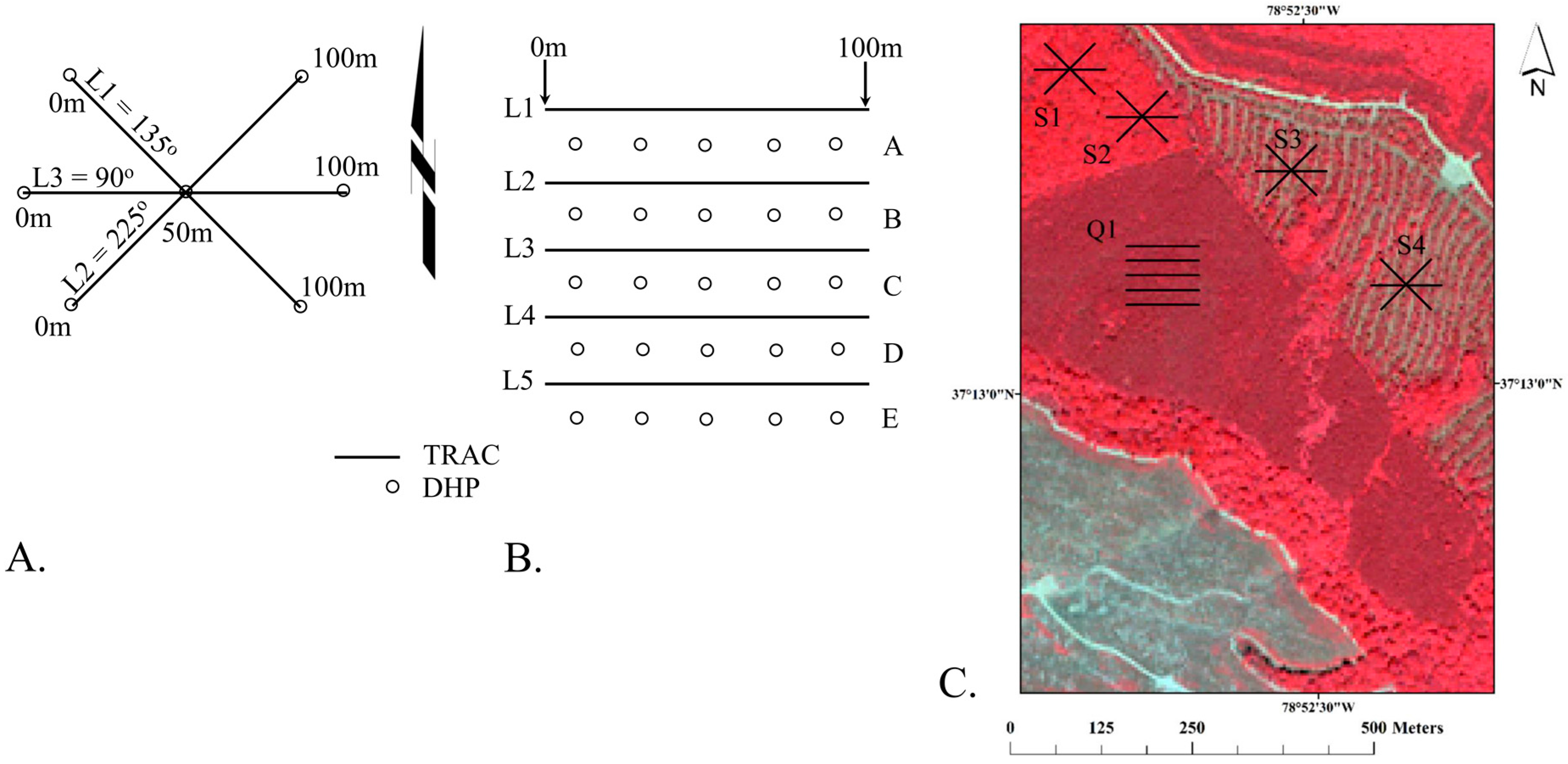
2.2. In Situ Measurements
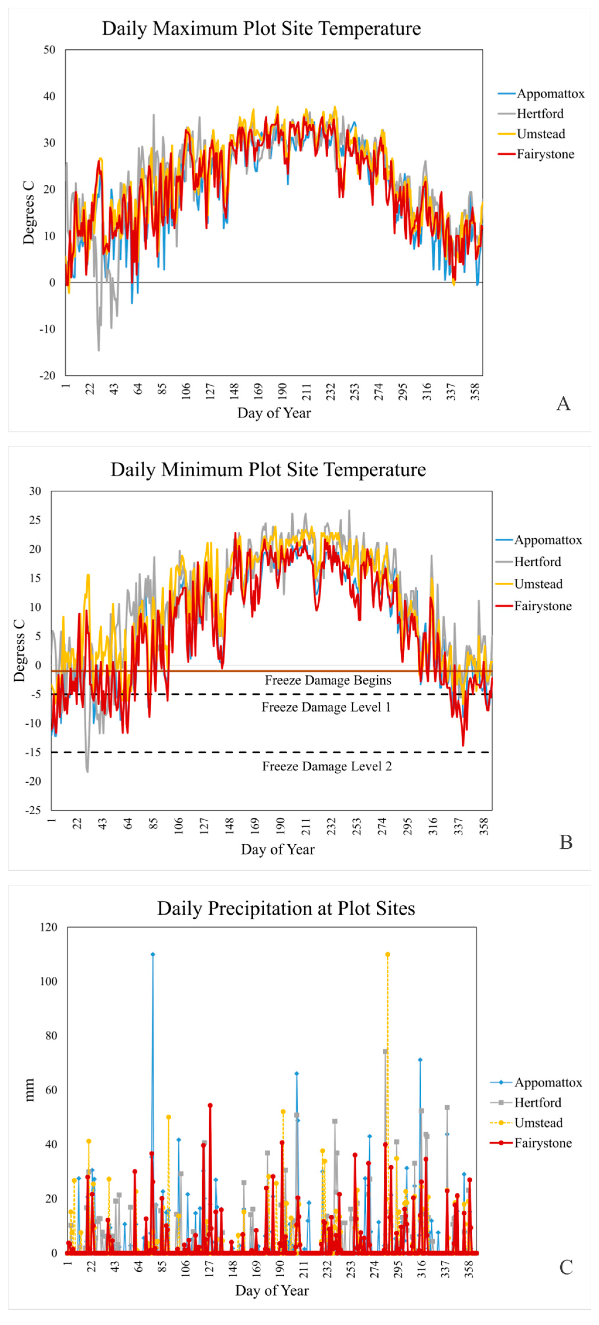
2.3. Soil and Meteorology
2.4. The EPIC Model
3. Results
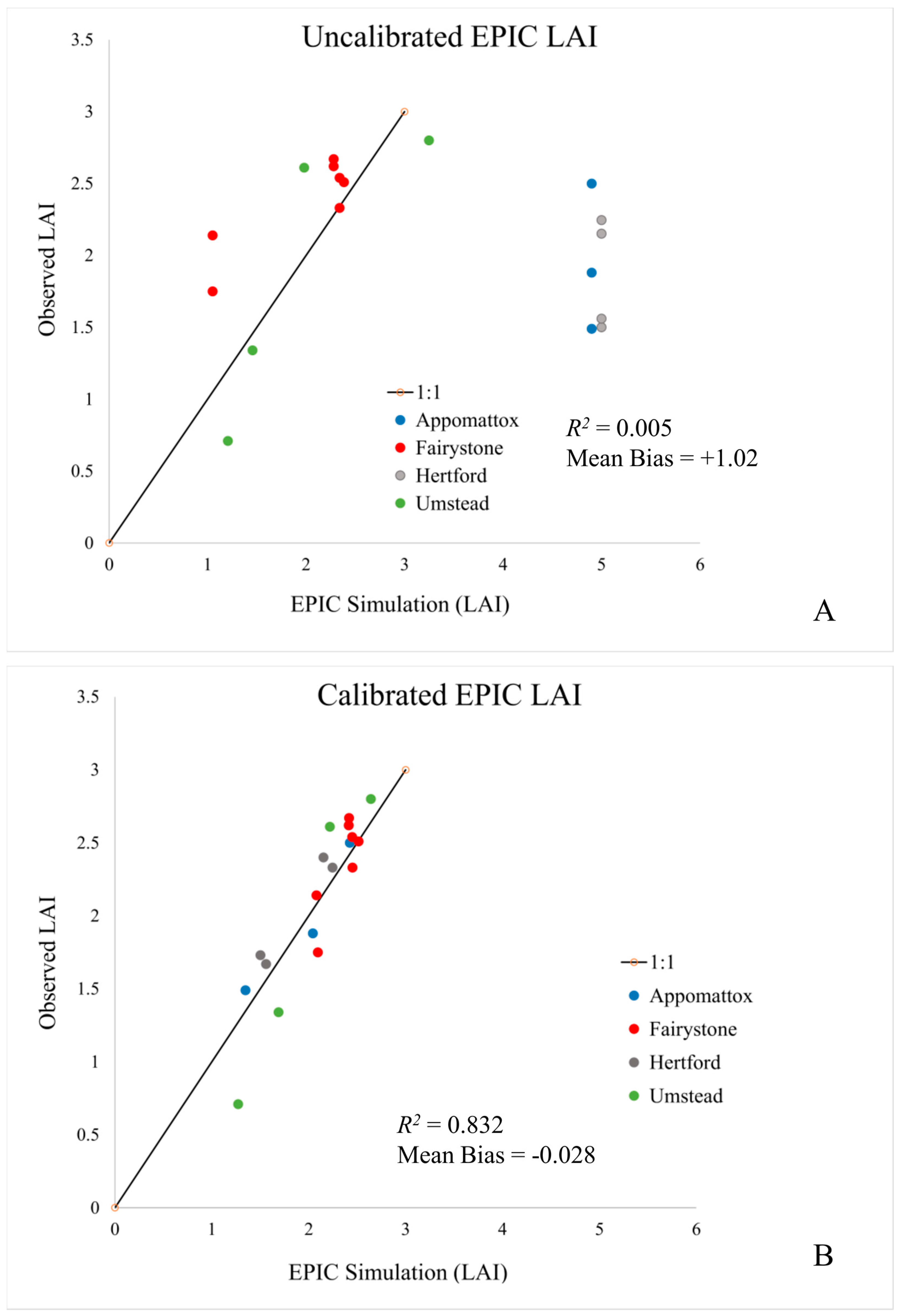
3.1. Model Calibration
3.2. Calibrated Model Results
3.2.1. Appomattox
3.2.2. Hertford
3.2.3. Fairystone
3.2.4. Umstead
4. Discussion
5. Conclusions
Supplementary Materials
Acknowledgments
Author Contributions
Conflicts of Interest
References
- Cooter, E.J.; Rae, A.; Bruins, R.; Schwede, D.; Dennis, R. The Role of the Atmosphere in the Provision of air-Ecosystem Services. Sci. Total Environ. 2013, 448, 197–208. [Google Scholar] [CrossRef] [PubMed]
- Black, T.A.; Chen, W.J.; Barr, A.G.; Arain, M.A.; Chen, Z.; Nesic, Z.; Hogg, E.H.; Neumann, H.H.; Yang, P.C. Increased carbon sequestration by a boreal deciduous forest in years with a warm spring. Geophys. Res. Lett. 2000, 27, 1271–1274. [Google Scholar] [CrossRef]
- Karl, T.; Harley, P.; Emmons, L.; Thornton, B.; Guenther, A.; Basu, C.; Turnipseed, A.; Jardine, K. Efficient atmospheric cleansing of oxidized organic trace gases by vegetation. Science 2010, 330, 816–819. [Google Scholar] [CrossRef] [PubMed]
- Nichol, J.; Wong, M.S. Estimation of ambient BVOC emissions using remote sensing techniques. Atmos. Environ. 2011, 45, 2937–2943. [Google Scholar] [CrossRef]
- Levis, S.; Foley, J.A.; Pollard, D. Potential high-latitude vegetation feedbacks on CO2-induced climate change. Geophys. Res. Lett. 1999, 26, 747–750. [Google Scholar] [CrossRef]
- Stull, R.B. An Introduction to Boundary Layer Meteorology; Kluwer Academic Publishers: Dordrecht, The Netherlands, 1988; pp. 1–665. [Google Scholar]
- Byun, D.W.; Schere, K.L. Review of the governing equations, computational algorithms, and other components of the models-3 Community Multiscale Air Quality (CMAQ) modeling system. Appl. Mech. Rev. 2006, 59, 51–77. [Google Scholar] [CrossRef]
- Meyers, T.P.; Finkelstein, P.; Clarke, J.; Ellestad, T.G.; Sims, P.F. Description and evaluation of a multilayer model for inferring dry deposition using standard meteorological measurements. J. Geophys. Res. 1998, 103, 22645–22661. [Google Scholar] [CrossRef]
- Pleim, J.; Ran, L. Surface Flux Modeling for Air Quality Applications. Atmosphere 2011, 2, 271–302. [Google Scholar] [CrossRef]
- Sickles, J.E.; Shadwick, D.E. Air quality and atmospheric deposition in the eastern US: 20 years of change. Atmos. Chem. Phys. 2015, 5, 173–197. [Google Scholar] [CrossRef]
- Dentener, F.; Vet, R.; Dennis, R.L.; Du, E.; Kulshretha, U.C.; Galy-Lacaus, C. Progress in Monitoring and Modelling Estimates of Nitrogen Deposition at Local, Regional and Global Scales. In Nitrogen Deposition, Critical Loads and Biodiversity; Sutton, M.A., Mason, K.E., Sheppard, L.J., Sverdrup, H., Haeuber, R., Hicks, K.W., Eds.; Springer: Dordrecht, The Netherlands, 2014; pp. 7–22. [Google Scholar]
- Cooter, E.; Schwede, D. Sensitivity of the National Oceanic and Atmospheric Administration multilayer model to instrument error and parameterization uncertainty. J. Geophys. Res. 2000, 105, 6695–6707. [Google Scholar] [CrossRef]
- Skamarock, W.C.; Klemp, J.B.; Dudhia, J.; Gill, D.O.; Barker, D.M.; Duda, M.G.; Huang, X.-Y.; Wang, W.; Powers, J.G. A Description of the Advanced Research WRF Version 3; National Center for Atmospheric Research: Boulder, CO, USA, 2008; p. 125. [Google Scholar]
- Pleim, J.E.; Xiu, A.; Finkelstein, P.L.; Otte, T.L. A coupled land-surface and dry deposition model and comparison to field measurements of surface heat, moisture and ozone fluxes. Water Air Soil Pollut. Focus 2001, 1, 243–252. [Google Scholar] [CrossRef]
- Ran, L.; Gilliam, R.; Binkowski, F.S.; Xiu, A.; Pleim, J.; Band, L. Sensitivity of the WRF/CMAQ modeling system to MODIS LAI, FPAR, and albedo. J. Geophys. Res. Atmos. 2015, 120, 8491–8511. [Google Scholar] [CrossRef]
- Bonan, G.B.; Oleson, K.W.; Fisher, R.A.; Lasslop, G.; Reichstein, M. Reconciling leaf physiological traits and canopy flux data: Use of the TRY and FLUXNET databases in the Community Land Model version 4. J. Geophys. Res. G Biogeosci. 2012, 117. [Google Scholar] [CrossRef]
- Lloyd, J.; Patiño, S.; Paiva, R.Q.; Nardoto, G.B.; Quesada, C.A.; Santos, A.J.B.; Baker, T.R.; Brand, W.A.; Hilke, I.; Gielmann, H.; et al. Optimization of photosynthetic carbon gain and within-canopy gradients of associated foliar traits for Amazon forest trees. Biogeosciences 2010, 7, 1833–1859. [Google Scholar] [CrossRef]
- Mercado, L.; Lloyd, J.; Carswell, F.; Malhi, Y.; Meir, P.; Nobre, A.D. Modelling Amazonian forest eddy covariance data: A comparison of big leaf versus sun/shade models for the C-14 tower at Manaus I. Canopy photosynthesis. Acta Amazon. 2006, 36, 69–82. [Google Scholar] [CrossRef]
- Mercado, L.M.; Lloyd, J.; Dolman, A.J.; Sitch, S.; Patiño, S. Modelling basin-wide variations in Amazon forest productivity—Part 1: Model calibration, evaluation and upscaling functions for canopy photosynthesis. Biogeosciences, 2009, 6, 1247–1272. [Google Scholar] [CrossRef]
- Goto, Y. Improved Vegetation Characterization and Freeze Statistics in a Regional Spectral Model for the Florida Citrus Farming Region. Ph.D. Thesis, The Florida State University, Tallahassee, FL, USA, 2008. [Google Scholar]
- Ran, L.; Pleim, J.; Gilliam, R.; Binkowski, F.S.; Hogrefe, C.; Band, L. Improved meteorology from an updated WRF/CMAQ modeling system with MODIS vegetation and albedo. J. Geophys. Res. 2016, 121, 2393–2415. [Google Scholar] [CrossRef]
- Opie, J.E. Predictability of Individual Tree Growth Using Various Definitions of Competing Basal Area. For. Sci. 1968, 14, 314–323. [Google Scholar]
- Chen, J.M.; Black, T.A. Foliage area and architecture of plant canopies from sunfleck size distributions. Agric. For. Meteorol. 1992, 60, 249–266. [Google Scholar] [CrossRef]
- Iiames, J.S.; Congalton, R.G.; Pilant, A.N.; Lewis, T.E. Validation of an integrated estimation of Loblolly pine (Pinus taeda L.) leaf area index (LAI) utilizing two indirect optical methods in the southeastern United States. South. J. Appl. For. 2008, 32, 101–110. [Google Scholar]
- Leblanc, S.G. DHP-TRACWin Manual; Canada Centre for Remote Sensing, Natural Resources Canada: Ottawa, ON, Canada, 2008.
- Frazer, G.W.; Canham, C.D.; Lertzman, K.P. Gap Light Analyzer (GLA), Version 2.0: Imaging Software to Extract Canopy Structure and Gap Light Transmission Indices from True-Color Fisheye Photographs, User’s Manual and Program Documentation; Simon Fraser University: Burnaby, BC, Canada; The Institute of Ecosystem Studies: Millbrook, New York, NY, USA, 1999. [Google Scholar]
- Kiniry, J.R.; Williams, J.R.; Gassman, P.W.; Debaeke, P. A general, process-oriented model for two competing plant species. Trans. ASAE 1992, 35, 801–810. [Google Scholar] [CrossRef]
- Kiniry, J.R.; Macdonald, J.D.; Kemanian, A.R.; Watson, B.; Putz, G.; Prepas, E.E. Plant growth simulation for landscape-scale hydrological modelling. Hydrol. Sci. J. 2008, 53, 1030–1042. [Google Scholar] [CrossRef]
- MacDonald, J.D.; Kiniry, J.R.; Putz, G.; Prepas, E.E. A multi-species, process based vegetation simulation module to simulate successional forest regrowth after forest disturbance in daily time step hydrological transport models. J. Envrion. Eng. 2008, 7, 127–143. [Google Scholar] [CrossRef]
- Gassman, P.W.; Reyes, M.R.; Green, C.H.; Arnold, J.G. The soil and water assessment tool: Historical development, applications, and future research directions. Trans. ASABE 2007, 504, 1211–1250. [Google Scholar] [CrossRef]
- Putz, G.; Burke, J.M.; Smith, D.W.; Chanasyk, D.S.; Prepas, E.E.; Mapfuma, E. Modelling the effects of boreal forest landscape management upon streamflow and water quality: Basic concepts and considerations. J. Environ. Eng. Sci. 2003, 2, S87–S101. [Google Scholar] [CrossRef]
- Arnold, J.G.; Fohrer, N. SWAT2000: Current capabilities and research opportunities in applied watershed modelling. Hydrol. Process. 2005, 19, 563–572. [Google Scholar] [CrossRef]
- WWilliams, J.W.; Izaurralde, R.C.; Steglich, E.M. Agricultural Policy/Environmental eXtender Model Theoretical Documentation Version 0806; Blackland Research and Extension Center: Temple, TX, USA, 2012; pp. 1–131. Available online: http://epicapex.tamu.edu/files/2014/10/APEX0806-theoretical-documentation.pdf (accessed on 31 October 2017).
- McIntyre, B.D.; Riha, S.J.; Ong, C.K. Light interception and evapotranspiration in hedgerow agroforestry systems. Agric. For. Meteorol. 1996, 81, 31–40. [Google Scholar] [CrossRef]
- Saleh, A.; Willimas, J.R.; Wood, J.C.; Hauck, L.M.; Blackburn, W.H. Application of APEX for Forestry. Trans. ASAE 2004, 47, 751–765. [Google Scholar] [CrossRef]
- Wang, X.; Saleh, A.; McBroom, M.W.; Williams, J.R.; Yin, L. Test of APEX for Nine Forested Watersheds in East Texas. J. Environ. Qual. 2007, 36, 983–995. [Google Scholar] [CrossRef] [PubMed]
- Monsi, M.; Saeki, T. Uber den lichtfaktor in den pflanzengesellschaften und seine bedeutung fur die stoffproduction. Jpn. J. Bot. 1953, 14, 22–52. [Google Scholar]
- United States Department of Agriculture Forest Service. Silvics of North America: 1. Conifers; 2. Hardwoods. Agriculture Handbook 654; U.S. Department of Agriculture, Forest Service: Washington, DC, USA, 1990; Volume 2, pp. 1–877.
- Guo, T.; Engel, A.; Shao, G.; Arnold, J.G.; Srinivasn, R.; Kiniry, J.R. Functional approach to simulating short-rotation woody crops in process-based models. BioEnergy Res. 2015, 8, 1598–1613. [Google Scholar] [CrossRef]
- Loudermilk, E.L.; Hiers, K.; Pokswinski, S.; O’Brian, J.J.; Barnett, A.; Mitchell, R.J. The path back: Oaks (Quercus spp.) facilitate longleaf pine (Pinus Palustris) seedling establishment in xeric sites. Ecosphere 2016, 7, E01361. [Google Scholar] [CrossRef]
- Baker, K.; Woody, M.; Tonnesen, G.; Hutzell, W.; Pye, H.; Beaver, M.; Pouliot, G.; Peirce, T. Contribution of regional-scale fire events to ozone and PM 2.5 air quality estimated by photochemical modeling approaches. Atmos. Environ. 2016, 140, 539–554. [Google Scholar] [CrossRef]
- Cooter, E.J.; Bash, J.O.; Benson, V.; Ran, L. Linking agricultural crop management and air quality models for regional national-scale nitrogen assessments. Biogeosciences 2012, 9, 4023–4035. [Google Scholar] [CrossRef]
- Scheller, R.M.; Mladenoff, D.J. A forest growth and biomass module for a landscape simulation model, LANDIS: Design, validation, and application. Ecol. Model. 2004, 180, 211–229. [Google Scholar] [CrossRef]
- Creutzburg, M.K.; Scheller, R.M.; Lucash, M.S.; LeDuc, S.D.; Johnson, M.G. Forest management scenarios in a changing climate: Trade-offs between carbon, timber, and old forest. Ecol. Appl. 2017, 27, 503–518. [Google Scholar] [CrossRef] [PubMed]
- Morisette, J.; Privette, J.L.; Baret, F.; Myneni, R.B.; Nickeson, J.; Garrigues, S.; Shabanov, N.; Fernandes, R.; Leblanc, S.; Kalacska, M.; et al. Validation of global moderate-resolution LAI products: A framework proposed within CEOS Land Product Validation Subgroup. IEEE Geosci. Remote Sens. 2006, 44, 1804–1817. [Google Scholar] [CrossRef]
- Iiames, J.S.; Congalton, R.G.; Lewis, T.E.; Pilant, A.E. Uncertainty analysis in the creation of a fine-resolution leaf area index (LAI) reference map for validation of moderate resolution LAI products. Remote Sens. 2015, 7, 1397–1421. [Google Scholar] [CrossRef]


| Stand Site | Lat/Long | Elev. (m) | Coop Site | Lat/Long | Elev. (m) | Dist. (km) |
|---|---|---|---|---|---|---|
| Appomattox | 37.22, −78.88 | 200 | Appomattox, VA/51011 | 37.36, −78.83 | 277.4 | 15.8 |
| Hertford | 36.38, −77.00 | 10 | Jackson, NC/374456 | 36.40, −77.42 | 39.6 | 37.9 |
| Fairystone | 36.77, −80.09 | 470 | Martinsville, VA/515300 | 36.71, −79.87 | 231 | 21 |
| Umstead | 35.86, −78.74 | 94 | Raleigh, NC/377079 | 35.79, −78.70 | 121.9 | 8.2 |
| Tree Species | Water (Days) | Nitrogen (Days) | Temperature (Days) |
|---|---|---|---|
| Loblolly pine | 39 | 1 | 125 |
| Sweetgum | 39 | 1 | 190 |
| White oak | 37 | 0 | 208 |
| Red maple | 41 | 0 | 125 |
| Site | Quad | Date | LAI (Mean) | LAI (Std Dev) |
|---|---|---|---|---|
| Fairystone | Q1 | 1-May | 2.14 | 0.24 |
| Q2 | 1-May | 1.75 | 0.35 | |
| Q1 | 25-June | 2.62 | 0.32 | |
| Q2 | 25-June | 2.67 | 0.38 | |
| Q3 | 8-July | 2.33 | 0.41 | |
| Q4 | 8-July | 2.54 | 0.35 | |
| Q4 | 1-September | 2.51 | 0.4 | |
| Umstead | Q1 | 5-April | 0.71 | 0.09 |
| Q1 | 13-April | 1.34 | 0.67 | |
| Q1 | 23-April | 2.61 | 0.49 | |
| Q1 | 21-October | 2.8 | 0.58 | |
| Appomattox | Q1 | 6-March | 1.49 | 0.13 |
| Q1 | 23-May | 1.88 | 0.18 | |
| Q1 | 30-July | 2.5 | 0.25 | |
| Q1 | 6-August * | 2.17 | 0.08 | |
| Hertford | Q1 | 5-March | 1.73 | 0.14 |
| Q1 | 9-April | 1.67 | 0.17 | |
| Q1 | 18-June | 2.4 | 0.32 | |
| Q1 | 25-July | 2.33 | 0.27 | |
| Q1 | 5-August * | 2.11 | 0.24 |
| Loblolly Pine | White Oak | Red Maple | Sweetgum | Chestnut Oak | Pignut Hickory | American Holly | Yellow Poplar | Black Oak | |
|---|---|---|---|---|---|---|---|---|---|
| Appomattox | C | C | C | C | |||||
| Bio Maturity (years) | 55 | 175 | 100 | 60 | |||||
| Normalized | 1246 | 1655 | 1805 | 150 | |||||
| Density (stems) | |||||||||
| Species % | 25.7 | 34.1 | 37.2 | 3 | |||||
| Stand Age | 19 | 19 | 19 | 19 | |||||
| Hertford | V | V | V | C | |||||
| Bio Maturity (years) | 55 | 100 | 60 | 100 | |||||
| Normalized | 1482 | 2862 | 668 | 1626 | |||||
| Density (stems) | |||||||||
| Species % | 22.3 | 43.1 | 10.1 | 24.5 | |||||
| Stand Age | 20 | 20 | 20 | 20 | |||||
| Fairystone | V | C | C | ||||||
| Bio Maturity (years) | 100 | 150 | 100 | ||||||
| Normalized Density (stems) | 120 | 307 | 39 | ||||||
| Species % | 25.7 | 65.9 | 8.4 | ||||||
| Stand Age | 80 | 80 | 80 | ||||||
| Umstead | V | C * | C | ||||||
| Bio Maturity (years) | 175 | 100 | 100 | ||||||
| Normalized | 184 | 1 | 86 | ||||||
| Density (stems) | |||||||||
| Species % | 30.5 | 0.1 | 14.3 | ||||||
| Stand Age | 80 | 80 | 80 |
| Timberland (Ha) | TPH | Age Class | Age Class | Age Class | |
|---|---|---|---|---|---|
| 1–20 year | 21–40 year | 41–60 year | |||
| % | % | % | |||
| Loblolly pine | 14,755 | 931 (52) | 100 | ||
| Virginia Pine | 3726 | 418 (24) | 100 | ||
| Mixed Oak | 12,007 | 90 (5) | 100 | ||
| Mixed upland hardwoods | 14,717 | 339 (19) | 100 | ||
| Total Forested | 18,294 | ||||
| Total Area | 32,170 |
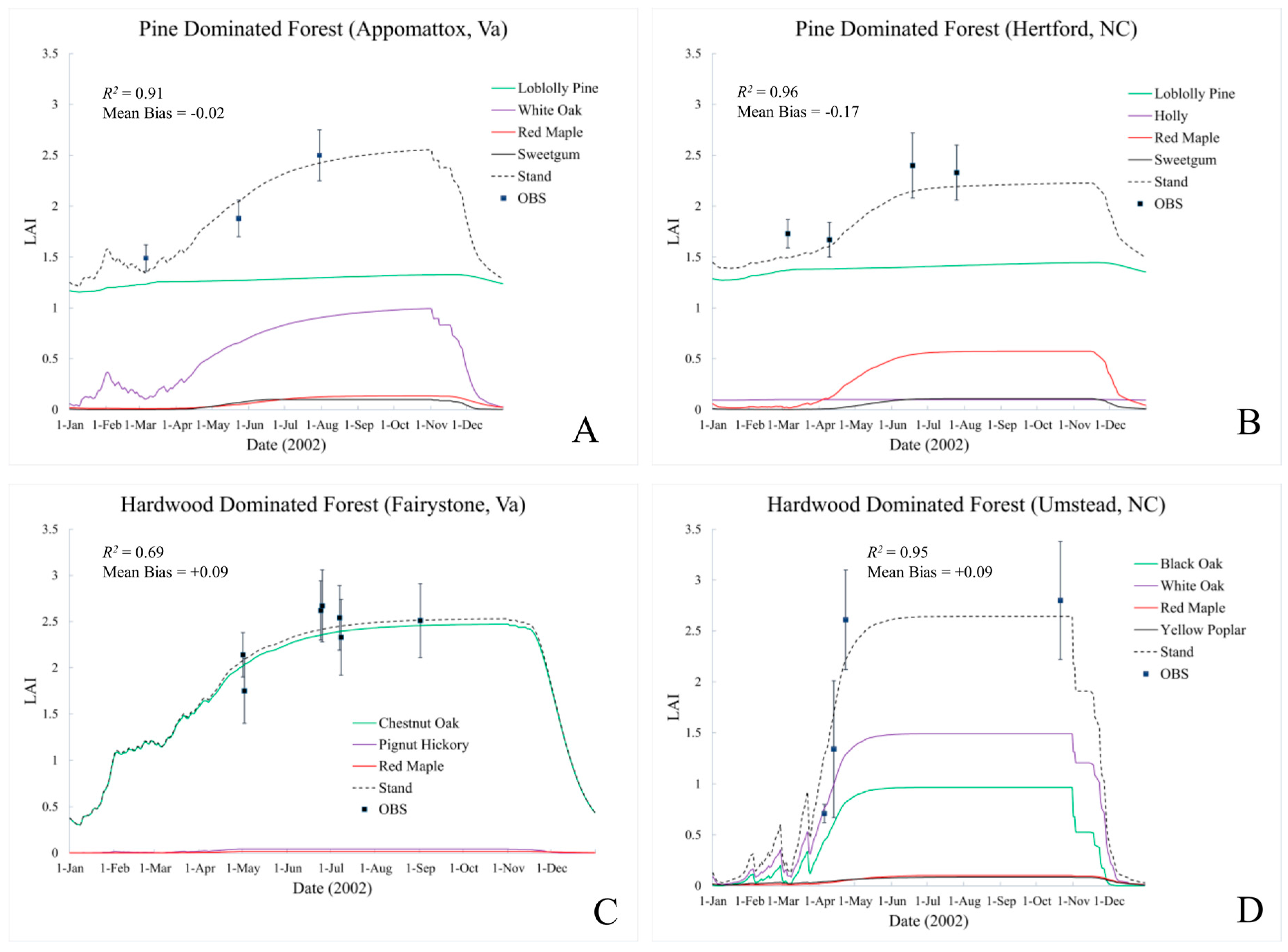
| Stand Site | Obs. | LAI R2 | LAI (Mean Bias) | Obs. Dominant Height (m) | EPIC Dominant Species Height (m) |
|---|---|---|---|---|---|
| Appomattox | 3 | 0.91 | −0.02 | 15.9 | 14.9, Loblolly Pine |
| Hertford | 5 | 0.96 | −0.17 | 14.3 | 17.1, Loblolly Pine |
| Fairystone | 7 | 0.69 | 0.09 | 14.6–22.1 | 18.0, Chestnut Oak |
| Umstead | 4 | 0.95 | 0.09 | 12.8 | 12.3, White Oak |
© 2018 by the authors. Licensee MDPI, Basel, Switzerland. This article is an open access article distributed under the terms and conditions of the Creative Commons Attribution (CC BY) license (http://creativecommons.org/licenses/by/4.0/).
Share and Cite
Iiames, J.S.; Cooter, E.; Schwede, D.; Williams, J. A Comparison of Simulated and Field-Derived Leaf Area Index (LAI) and Canopy Height Values from Four Forest Complexes in the Southeastern USA. Forests 2018, 9, 26. https://doi.org/10.3390/f9010026
Iiames JS, Cooter E, Schwede D, Williams J. A Comparison of Simulated and Field-Derived Leaf Area Index (LAI) and Canopy Height Values from Four Forest Complexes in the Southeastern USA. Forests. 2018; 9(1):26. https://doi.org/10.3390/f9010026
Chicago/Turabian StyleIiames, John S., Ellen Cooter, Donna Schwede, and Jimmy Williams. 2018. "A Comparison of Simulated and Field-Derived Leaf Area Index (LAI) and Canopy Height Values from Four Forest Complexes in the Southeastern USA" Forests 9, no. 1: 26. https://doi.org/10.3390/f9010026
APA StyleIiames, J. S., Cooter, E., Schwede, D., & Williams, J. (2018). A Comparison of Simulated and Field-Derived Leaf Area Index (LAI) and Canopy Height Values from Four Forest Complexes in the Southeastern USA. Forests, 9(1), 26. https://doi.org/10.3390/f9010026