Article

Developing Aboveground Biomass Equations Both Compatible with Tree Volume Equations and Additive Systems for Single-Trees in Poplar Plantations in Jiangsu Province, China

1
Ministry of Education Key Laboratory for Silviculture and Conservation, College of Forestry, Beijing Forestry University, Beijing 100083, China
2
Academy of Forest Inventory and Planning, State Forestry Administration, Beijing 100714, China
*
Author to whom correspondence should be addressed.
Forests 2016, 7(2), 32; https://doi.org/10.3390/f7020032
Submission received: 28 August 2015 / Revised: 22 December 2015 / Accepted: 25 January 2016 / Published: 29 January 2016

Abstract

:
We developed aboveground biomass equations for poplar plantations in Jiangsu Province, China, both compatible with tree volume equations and additive systems. Biomass equations were fitted with 80 selected and previously harvested sample trees. Additivity property was assured by applying a “controlling directly under total biomass proportion function” approach. Weighted regression was used to correct heteroscedasticity. Parameters were estimated using a nonlinear error-in-variable model. The results indicated that (1), on average, stems constituted the largest proportion (71.5%) of total aboveground biomass; (2) the aboveground biomass equations, both compatible with tree volume equations and additive systems, obtained good model fitting and prediction, of which the coefficient of determination ranged from 0.903 to 0.987, and the total relative error and the mean prediction error were less than 2.0% and 10.0%, respectively; (3) adding H and CW into the additive system of biomass equations did not improve model fitting and performance as expected, especially for branches and foliage biomass; and (4) the additive systems of biomass equations presented here provided more reliable and accurate biomass predictions than the independent biomass equations fitted by ordinary least square regression. This system of additive biomass equations will prove to be applicable for estimating biomass of poplar plantations in Jiangsu Province of China.

1. Introduction

The forest ecosystem plays an important role in the global carbon cycle and climate change [1,2]. Forest biomass estimation is an essential aspect of quantifying the carbon budget [3], as well as the changes in the forest ecosystem. There is also an increasing interest globally in forest biomass research. Undoubtedly, the most reliable method to determine tree biomass is harvesting and weighing of all trees or all their parts in the field [3], but it is destructive, time-consuming, costly and laborious, and can only be carried out in small areas [4,5]. A large number of allometric relationships between tree biomass or its components and diameter at breast height (DBH), tree height (H), crown width (CW) and other easily measurable tree variables have been established during the last decades [6,7]. Allometric models are useful for non-destructively predicting biomass, and it is often the preferred approach to accurately estimate biomass of individual trees, plots and even regions [8].
Because of its fast growth, high-yield and strong adaptability to environmental changes [9,10], poplar has become one of the most widely distributed afforestation tree genera in China with a high economic and ecological value. According to the 8th National Forest Inventory (NFI) data, poplar plantations are of high proportion (67.4%) of the total forested area in Jiangsu Province of China. Liu et al. [11] have reported that the carbon sequestration of poplar trees is almost 20 times higher than that of other tree species. So, we believe that poplar plantations can make a considerable contribution to Jiangsu’s terrestrial carbon cycle. Many studies on poplar biomass and carbon storage at different levels have been conducted since the 1980s in China [12,13,14], demonstrating that research on the biomass models of poplar plantations is of great significance to predicting potential biomass accumulation and timber production. A great number of equations for individual tree biomass prediction have been developed for poplar in China, but few studies have been done in Jiangsu Province. These equations are expressed as [12,13,14,15,16]: M = a DBH b H c, lg M = a lg (DBH 2 H) + b, M = a DBH b, M = a (DBH 2 H) b, ln M = a ln (DBH 2 H) + b, ln M = a ln DBH + b and ln M = a ln H + b, which can be classified into nonlinear (power-law relationship) fitting to raw data, and linear fitting to log-transformed data.
A common problem encountered in developing biomass equations is the very small sample size (usually less than 10 trees) used in many previous studies [12,13,15], which may reduce the model precision [17]. In addition, heteroscedasticity in biomass data [18] has frequently been ignored, which would lead to unreliable parameter estimates in biomass modeling. Moreover, previous studies have reported that biomass equations should ensure the biomass additivity; in other words, the sum of the predictions for the tree components equals the prediction for the whole tree [18,19,20]. Unfortunately, little attention has been devoted to the additivity of total biomass and biomass components for poplar trees in China. Since tree volume is available in NFI systems, converting tree volume to biomass through allometric models can be the most convenient and reliable approach to estimating forest biomass over large areas [21].
Therefore, the goals of this study were: (1) to construct one-, two- and three-variable compatible biomass equations with tree volume equations for poplar trees in Jiangsu Province of China; (2) to develop three systems of additive biomass equations for predicting total aboveground biomass and biomass of its components; and (3) to analyze the biomass allocation for different components of a single tree afterward. To achieve better parameter estimates, the weighted regression and the nonlinear error-in-variable simultaneous equations were adopted.

2. Material and Methods

2.1. Site Description

The study was conducted in Jiangsu Province (116°21′–121°55′ E, 30°46′–35°07′ N), which is located on the east coast of China, lying in the lower regions of both the Yangtze River and Huai River. The total area is approximately 102,600 km2. The land of Jiangsu Province is generally flat and low-lying. The elevation ranges from about 2 to 625 m a.s.l. Spanning across the subtropical and warm-temperate climate zones, Jiangsu Province has four distinct seasons with a temperate climate and moderate rainfall. The mean annual temperature is 15.3 °C, and the mean annual precipitation is 1030 mm. According to the reference of GB/T 17296-2009 [22], soil types vary and include brown soil, yellow soil, yellow-brown soil and paddy soil. By the end of 2011, the forest coverage of Jiangsu Province has reached 2,174,500 ha with 1,815,300 ha of woodland.

2.2. Tree Biomass Data

2.2.1. Selection of Sample Trees

The biomass data, consisting of 80 individual poplar trees in Jiangsu Province of China, were derived from destructive harvesting between August and October in 2011, excluding rainy days. These sample trees were selected according to 10 diameter classes of 2, 4, 6, 8, 12, 16, 20, 26, 32, and 38 cm equally. Within each diameter class, sample trees were distributed by 3–5 height classes as evenly as possible. Thus, the sampled trees were representative of poplar in Jiangsu Province. Before conducting the destructive sampling, DBH (i.e., at 1.30 m aboveground) and crown width (CW) were measured in the field. CW was determined by averaging measurements of a north-south axis with a diameter taken at 90 degrees (a west-east axis). Also, the tree height (H) was measured after felling. The aboveground tree material was then divided into stem wood, bark, branches and foliage components.

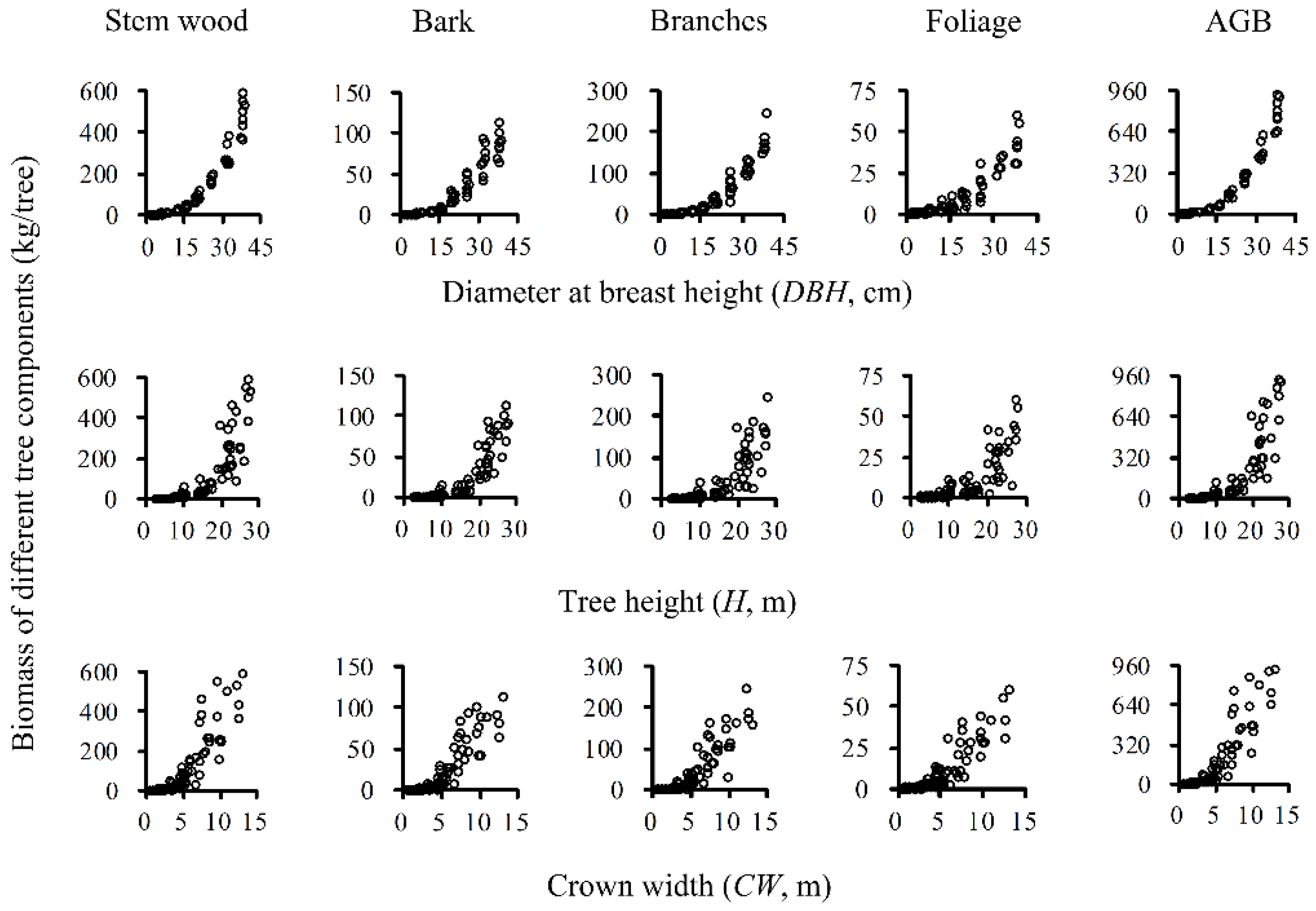
2.2.2. Biomass of Aboveground Tree Components

After removal of dead and living branches, the stem was divided into 11 sections at points corresponding to 0, 0.05, 0.1, 0.2, 0.3, 0.4, 0.5, 0.6, 0.7, 0.8 and 0.9 of tree height. Then, diameter of each section was measured. The top log was treated as a cone and the volume (Vtop) was calculated as 1/3 gl′, where g′ is the basal area of the top log, and l′ is the length of the top log. The remaining logs were treated as a paraboloid frustrum, and the Smalian’s formula was used to calculate the volume. The total tree volume was computed as the sum of the volume of each log. The stem was cut into three sections (top, middle, and bottom) and each section was weighed fresh in the field. Two 3-cm-thick discs were cut from both sides of each stem at a height of 10.0%, 35.0% and 70.0% for stem (stem wood + bark) biomass determination. Sample discs were partitioned into stem wood and bark as subsamples.
The crown (branches + foliage) incorporating branches (dead branches + living branches) and foliage was partitioned into three layers (top, middle and bottom) after felling of sample trees. Dead branches were firstly selected and weighed. Also, fresh weight of living branches for each layer was weighed. For each layer, three branches (with medium size, length and leaves) were selected and all leaves were removed. Branches (without leaves) and foliage within each layer were weighed respectively in the field. Subsamples of living branches without leaves were selected for three layers, while mixed subsamples of foliage were selected from all removed leaves. Besides, subsamples of dead branches were selected from dead sample branches.
Subsamples of different components were weighed fresh in the field. They were stored in plastic bags, and sent to the laboratory to determine the moisture content. Dry weights were obtained by drying subsamples at a temperature of 85 °C until a constant weight was achieved. The dry weights of samples were calculated by multiplying the fresh weight with the dry weight/fresh weight ratios of the corresponding subsamples. According to the ratios of dry weight to fresh weight, the total aboveground biomass was obtained by summing the dry weights of stem wood, bark, branches and foliage. The dry weight of the stem wood, bark, branches and foliage were calculated through fresh weight multiplied by dry weight/fresh weight ratio of the corresponding samples [8]. Total aboveground tree biomass (AGB) was estimated as the sum of the dry weight of stem wood, bark, branches and foliage. Tree variables and biomass of different tree components are summarized in Table 1.
Table 1. Tree characteristics and summary statistics of the aboveground biomass components for poplar (n = 80) in Jiangsu Province of China.
StatisticsTree VariablesBiomass of Different Aboveground Tree Components (kg)
DBH (cm)H (m)CW (m)Stem WoodBarkBranchesFoliageAboveground Tree
Mean16.414.15.0107.022.540.810.9181.1
Min.1.72.60.40.10.00.00.10.3
Max.38.627.613.0591.0113.9245.960.0921.7
S.D.11.77.63.2154.330.958.014.5254.7
Note: Minimum (Min.); maximum (Max.); standard deviation (SD.).

2.3. Independent Biomass Equations Development

Based on the destructively harvested biomass data, we plotted the relationships between biomass of total aboveground tree and its components per tree and tree variables (DBH, H and CW) in Figure 1, showing obvious nonlinear relationships.
Figure 1. The relationships between the biomass components versus tree level variables for poplar in Jiangsu Province of China (n = 80).
Forests 07 00032 g001
Considering our analysis above, we decided to use nonlinear regressions as base models to establish different biomass equations, relating biomass of total aboveground tree or its components to standing tree variables, such as DBH, H and CW [23,24,25] in this study. The base models were written as:
M = β 0 D B H β 1 + ε
M = β 0 D B H β 1 H β 2 + ε
M = β 0 D B H β 1 H β 2 C W β 3 + ε
where M is the biomass of different components of a tree (kg/tree), including stem wood, bark, branches, foliage and total aboveground tree; DBH (cm), H (m) and CW (m) are the independent variables; β0, β1, β2 and β3 are the allometric parameters; and ε is a random error which is assumed to be a normal distribution, N (0, σ2).

2.4. Nonlinear Error-in-Variable Model

Commonly, regression models are fitted by the ordinary least square (OLS), assuming that the independent variables are without errors and the dependent variables are with errors [26,27]. When both independent and dependent variables are assumed to have measurement errors, the OLS method is no longer adequate, and a measurement error model, the error-in-variable method, is introduced to such regressions [28]. According to Tang et al. [29], the nonlinear error-in-variable simultaneous equations can be described as follows:
{ f ( y i , x i , c ) = 0 Y i = y i + e i , i = 1 , 2 , n E ( e i ) = 0 , cov ( e i ) = σ 2 ψ
where xi is the observed value of q-dimensional error-free-variable, Yi is the observed value of p-dimensional error-in-variable, ƒ() is the m-dimensional vector function, yi is the unknown true value of Yi, and E(ei) is the expectation of error ei. The covariance matrix of error ei is denoted as ϕ = σ2ψ, where ψ is the structure matrix of error ei, and σ2 is the error of the estimate.

2.5. Compatible Biomass Equations Establishment

The compatible regression models [2] were used to determine the total aboveground biomass in this study. Firstly, one- and two-variable tree volume equations were fitted by the following regression functions:
V = α 0 D B H α 1 + ε
V = α 0 D B H α 1 H α 2 + ε
where V is the tree volume (m3), α0, α1 and α2 are parameters.
On this basis, the compatible regression models, reflecting relationships between tree volume and biomass, can then be expressed as follows:
M = γ 0 D B H γ 1 V + ε
M = γ 0 D B H γ 1 H γ 2 V + ε
M = γ 0 D B H γ 1 H γ 2 C W γ 3 V + ε
Here, M is the total aboveground biomass (kg/tree); γ0, γ1, γ2 and γ3 are parameters for the conversion function from tree volume to biomass. It should be noted that, in Equation (9), V is still the two-variable tree volume equation instead of the three-variable tree volume equation. Accordingly, we can yield the following relations:
β 0 = α 0 × γ 0 , β 1 = α 1 + γ 1 , β 2 = α 2 + γ 2 , β 3 = γ 3
To assure the regression parameter compatibility between total aboveground biomass and tree volume equations, i.e., Equation (10) is true, the nonlinear error-in-variable method was applied to develop three sets of nonlinear equations based on Equations (5) and (7) for one-variable models, Equations (6) and (8) for two-variable models, and Equations (6) and (9) for three-variable models, respectively, where DBH, H and CW were regarded as error-free-variables, and M and V as error-in-variables. Based on the tree volume and total aboveground biomass data of 80 sample poplar trees, three sets of compatible biomass equations were fitted by nonlinear error-in-variable simultaneous equations in the ForStat 2.1 [29].

2.6. Additive Biomass Equations Construction

A “controlling directly under total biomass by proportion function” approach, which separates total biomass from component biomass (stem wood, bark, branches and foliage) and satisfies the additivity property (i.e., the predictions of four components biomass sum to the total biomass), was presented to design the additive system of biomass equations [30]. Firstly, the nonlinear biomass equations for four tree components (stem wood, bark, branches and foliage) were fitted independently, and the weighting factor of each component was adopted in the additive systems. Then, let f0(x) represent the total aboveground biomass of a tree (kg/tree), which was fitted independently of this system by modeling compatible biomass equations with tree volume equations. f0(x) for one-, two- and three-variable models can be written as:
f 0 ( x ) = a 0 D B H b 0
f 0 ( x ) = a 0 D B H b 0 H c 0
f 0 ( x ) = a 0 D B H b 0 H c 0 C W d 0
where a0, b0, c0 and d0 are the parameters for f0(x), and a0 = β0, b0 = β1, c0 = β2 and d0 = β3.
Next, it is assumed that the relative proportions of stem wood, bark, branches and foliage to total biomass are g1(x), g2(x), 1 and g3(x), respectively. The relative proportion function gi(x) for one-, two- and three-variable models can be determined as:
g i ( x ) = a i D B H b i
g i ( x ) = a i D B H b i H c i
g i ( x ) = a i D B H b i H c i C W d i
where ai, bi, ci and di (i = 1, 2, 3) are the parameters for gi(x).
Finally, the structural equations for the system of additive biomass models can be specified as:
{ y 1 = g 1 ( x ) 1 + g 1 ( x ) + g 2 ( x ) + g 3 ( x ) × f 0 ( x ) y 2 = g 2 ( x ) 1 + g 1 ( x ) + g 2 ( x ) + g 3 ( x ) × f 0 ( x ) y 3 = 1 1 + g 1 ( x ) + g 2 ( x ) + g 3 ( x ) × f 0 ( x ) y 4 = g 3 ( x ) 1 + g 1 ( x ) + g 2 ( x ) + g 3 ( x ) × f 0 ( x )
where y1, y2, y3, y4 are the biomass of stem wood, bark, branches and foliage of a tree (kg/tree); x are DBH, H and CW.
Parameters of the system were estimated simultaneously by applying the nonlinear error-in-variable method in Forstat 2.1 [29]. Hence, we can guarantee that (i) the tree volume and aboveground biomass equations were compatible and (ii) the additive system of biomass equations meet the biomass “additivity” requirement.
Noting that, in the additive system of biomass equations, the relative ratio of branches’ biomass to total aboveground biomass was assumed to be 1. Why did we choose branches rather than stem wood, bark or foliage? If we assumed the relative proportion of stem wood (or bark, or foliage) biomass to total aboveground biomass was 1, did it make any difference? To make comparisons with the “branches”, actually, we established another three structural systems of additive biomass equations, and denoted as the “stem wood system”, “bark system” and “foliage system”, respectively. Also, the goodness-of-fit statistics for different systems of additive biomass equations were computed subsequently.

2.7. Heteroscedasticity Correction

As Parresol [18] discusses, normally biomass and volume data exhibit obvious heteroscedasticity; hence, it is necessary to take some countermeasures to eliminate the impact of heteroscedasticity. So far, the use of logarithmic transformation and weighted regression are two common approaches to calculate the model parameters in forest science [23,25]. In this paper, we applied weighted regression to correct bias in parameter estimates. Initially, the nonlinear regression models were fitted independently by the OLS method. Then, the weight factor of each model was determined as w = 1/DBH q, deriving from the regression relationship between DBH and residual squares (e2) of the OLS estimates, e2 = p × DBH q, where p, q are parameters. Finally, we fitted the nonlinear models by multiplying the weight factor (w = 1/DBH q) to both sides of the models.

2.8. Model Evaluation

The best-fit models were selected based on four goodness-of-fit statistics, the coefficient of determination (R2), standard error of estimate (SEE), total relative error (TRE), and mean prediction error (MPE) [18,31].
The coefficient of determination:
R 2 = 1 i = 1 n ( y i y ^ i ) 2 / i = 1 n ( y i y ¯ )
Standard error of estimate:
S E E = i = 1 n ( y i y ^ i ) 2 / ( n p )
Total relative error:
T R E = i = 1 n ( y i y ^ i ) / i = 1 n y ^ i × 100 %
Mean prediction error:
M P E = t α × ( S E E / y ¯ ) / n × 100 %
where y i is the observed value, y ^ i is the value calculated with the model, y ¯ is the mean observed value for one sample, n is the number of sample trees, p is the number of parameters, and tα is the t value at confidence level α with np degrees of freedom (tα ≈ 1.98 for α = 0.05).
To the best of our knowledge, ideally, an independent dataset is required to further evaluate the accuracy or applicability of the final biomass models [25]. Traditionally, a split-sample approach, which partitions the dataset into two portions, was applied for model assessment. In recent years, however, some researches have argued and claimed that the split-sample method did not provide any additional information about the parameter estimate and is a waste of money [32,33]. Therefore, it is strongly recommended that, in current study, we develop biomass models of the total tree and its components utilizing the full dataset, instead of splitting the dataset into a “fit dataset” and “validation dataset”. Additionally, to see whether the additive system of biomass equations is superior to independent equations, ratios of R2, SEE, TRE and MPE of system equation to that of the independent equation were calculated for each tree component and total aboveground biomass [17,20].

3. Results

3.1. Sample Tree Characterization

According to the mean biomass values of different tree components (Table 1), we computed the proportion of biomass of different tree components to total aboveground tree biomass. Accordingly, 59.1% of total aboveground biomass was allocated to the stem wood, 12.4% to the bark, 22.5% to the branches and 6.0% to the foliage. The ratio of stem biomass to total aboveground biomass was 71.5%.

3.2. Independent Biomass Equations

Parameters and goodness-of-fit statistics of one-, two- and three-variable biomass equations for different tree components are described in Table 2. In general, R2 values were above 0.90 for all biomass models. For total aboveground tree and stem wood, SEE and MPE generally decreased with the addition of variables H and CW. However, for bark, SEE and MPE decreased with the addition of H and showed a small increase with the inclusion of CW. On the contrary, for branches and foliage, SEE and MPE increased with the addition of H while there was a small decrease with the inclusion of CW. The total relative errors (TRE, in %) were less than 2.0% for all tree components, while the mean prediction errors (MPE, in %) ranged from 3.7% to 9.6%.
Table 2. Parameters and goodness-of-fit statistics for the biomass of different components estimated for an individual tree (n = 80).
ComponentsModelsParameters (p < 0.05)Goodness-of-Fit Statistics
β0β1β2β3R2SEE (kg)TRE (%)MPE (%)
M0One-variable0.0532.637//0.97641.21.55.0
Two-variable0.0242.4290.490/0.98631.0−0.03.7
Three-variable0.0212.4800.521−0.0640.98730.60.03.7
M1One-variable0.0222.752//0.96431.60.66.2
Two-variable0.0082.3630.743/0.97924.00.04.7
Three-variable0.0062.4900.784−0.1280.98123.20.04.6
M2One-variable0.0072.611//0.9149.0−0.39.0
Two-variable0.0042.0600.775/0.9427.41.87.4
Three-variable0.0042.1100.766−0.0540.9427.51.97.5
M3One-variable0.0072.784//0.96110.9−0.56.3
Two-variable0.0113.159−0.569/0.95012.4−0.77.1
Three-variable0.0103.170−0.505−0.0790.95212.2−0.47.0
M4One-variable0.0172.133//0.9054.50.39.2
Two-variable0.0242.407−0.402/0.9004.70.19.6
Three-variable0.0302.147−0.4060.3020.9024.60.29.5
Note: M0, M1, M2, M3, M4 are respectively the biomass of total aboveground tree, stem wood, bark, branches and foliage. The coefficient of determination (R2); standard error of estimate (SEE); total relative error (TRE); mean prediction error (MPE). For one-variable equations, the weight factors were 1/DBH2.14, 1/DBH2.03, 1/DBH1.82, 1/DBH2.05 and 1/DBH1.28 for M0–M4, respectively; for two-variable equations, the weight factors were 1/DBH1.51, 1/DBH1.61, 1/DBH2.35, 1/DBH2.15 and 1/DBH1.18 for M0–M4, respectively; for three-variable equations, the weight factors were 1/DBH1.42, 1/DBH1.45, 1/DBH2.35, 1/DBH1.99 and 1/DBH1.20 for M0–M4, respectively.

3.3. Compatible Biomass Equations

Parameters and goodness-of-fit statistics of three sets of equations for compatible tree volume and aboveground biomass are given in Table 3 and Table 4. As shown in Table 4, R2 values were all above 0.97 for biomass and volume equations. TRE and MPE values for all biomass and volume equations were both less than 5.0%. For two- and three-variable biomass equations, the four goodness-of-fit statistics were not very different, which provided slightly better results than one-variable equations, with higher R2 and lower SEE, TRE and MPE values.
Table 3. Parameters for compatible tree volume and aboveground biomass equations.
ModelsVolume ParametersBiomass ParametersConversion Functions
α0α1α2β0β1β2β3γ0γ1γ2γ3
One-variable0.1412.473/0.0522.642//0.3690.169//
Two-variable0.0552.0040.8230.0242.4220.499/0.4340.418−0.324/
Three-variable ///0.0222.4300.529−0.0200.4080.429−0.302−0.020
Note: The significant level (p < 0.05). The weight factors were 1/DBH2.43 and 1/DBH1.36 for one- and two-variable tree volume equations. The weight factors for total aboveground biomass were the same with Table 2. α0, α1 and α2 are parameters for tree volume equations; β0, β1, β2 and β3 are parameters for compatible biomass equations; γ0, γ1, γ2 and γ3 are parameters for conversion functions. For the three-variable compatible model, the two-variable tree volume equation instead of the three-variable tree volume equation was used here.
Table 4. Goodness-of-fit statistics for compatible tree volume and aboveground biomass equations.
ModelsTree VolumeAboveground Biomass
R2SEE (m3)TRE (%)MPE (%)R2SEE (kg)TRE (%)MPE (%)
One-variable0.9740.060.64.80.97641.01.34.9
Two-variable0.9910.040.02.90.98630.90.03.7
Three-variable////0.98730.60.03.7
Note: the coefficient of determination (R2); standard error of estimate (SEE); total relative error (TRE); mean prediction error (MPE). For the three-variable compatible model, the two-variable tree volume equation instead of the three-variable tree volume equation was used here.

3.4. Additive Biomass Equations

Four systems of additive biomass equations—the “stem wood system”, “bark system”, “branches system” and “foliage system”—were constructed and compared according to the goodness-of-fit statistics (Table 5). We found that the values of the goodness-of-fit statistics of the “stem wood system” and “bark system” of additive biomass equations were exactly the same, while those of the remaining two systems of additive biomass equations were also the same. To sum up, the “branches system” or “foliage system” performed a little better than the “stem wood system” or “bark system”. Therefore, using either the “branches system” or “foliage system” can obtain the best results.
Table 5. Goodness-of-fit statistics for different systems of additive biomass equations.
ComponentsModelsBranches or Foliage SystemStem Wood or Bark System
R2SEE (kg)TRE (%)MPE (%)R2SEE (kg)TRE (%)MPE (%)
M1One-variable0.96132.61.96.40.96132.61.96.4
Two-variable0.97924.20.04.80.97824.6−0.04.9
Three-variable0.98023.80.04.70.97924.20.04.8
M2One-variable0.9178.80.78.80.9178.80.78.8
Two-variable0.9457.30.67.30.9467.20.67.2
Three-variable0.9447.40.17.40.9457.30.17.3
M3One-variable0.96210.80.26.20.96210.80.26.2
Two-variable0.95611.7−0.46.70.95611.6−0.46.7
Three-variable0.95711.6−0.06.70.95811.5−0.06.6
M4One-variable0.9034.50.29.30.9034.50.29.3
Two-variable0.9034.60.09.40.9104.40.59.0
Three-variable0.9034.60.09.40.9094.50.19.1
Note: “Branches or Foliage System” assumed the relative ratio of branches or foliage biomass to total aboveground biomass was 1; while “Stem Wood or Bark System” assumed the relative ratio of stem wood or bark biomass to total aboveground biomass was 1.
To be consistent with the methods section, only the “branches system” of additive biomass equations was analyzed in detail. Parameters for the “branches system” of additive biomass equations with one, two and three independent variables are shown in Table 6. In practice, however, parameters for f0(x) were directly sourced from the compatible biomass equations as shown in Table 3. It can be seen from Table 6 that the addition of H has no effect on g3(x), and the inclusion of CW has no effect on gi(x) (i = 1, 2, 3).
Table 6. Parameters for the “branches system” of additive biomass equations.
Modelsf0(x)gi(x)Parameters (p < 0.05)
a1b1c1d1a2b2c2d2a3b3c3d3
One-variable(11)(14)3.434−0.054//1.118−0.198//2.484−0.647//
Two-variable(12)(15)0.970−0.7151.136/0.432−1.0611.246/1.778−0.549//
Three-variable(13)(16)0.837−0.6671.133/0.437−1.0161.194/1.761−0.545//
Note: f0(x) was the total aboveground biomass equation; gi(x) was the proportion function, g1(x), g2(x) and g3(x) were defined as the relative proportions of stem wood, bark and foliage to total biomass; a1, b1, c1, d1 are the parameters for g1(x), a2, b2, c2, d2 are the parameters for g2(x) and a3, b3, c3, d3 are the parameters for g3(x); the weight factors for total aboveground biomass and each component biomass were the same as in Table 2.
The goodness-of-fit statistics of the “branches system” of additive biomass equations are shown in Table 5. All biomass equations performed well (R2 ≥ 0.90). Compared to one-variable models, for stem wood and bark, R2 values of two- and three-variable models improved slightly; while for branches and foliage, there was no significant difference for R2 values of one-, two- and three-variable models. For all models, TRE values were less than 2.0%, and MPE values ranged from 4.7% to 9.4%. For stem wood, SEE and MPE generally decreased with the addition of variable H and CW; on the contrary, for foliage, the trend was that of an increase. Unlike with stem wood and foliage, for bark, SEE and MPE decreased with the addition of H and showed a small increase with the inclusion of CW; but the trend for branches was exactly opposite to bark.
In comparison to the independent equations which separately fit the biomass equations for the total tree and its components using OLS and weighted regression, the additive system of biomass equations provided a slight improvement in most of the goodness-of-fit statistics (Table 7). Values of the R2 ratio were generally greater than 1 for all components, excluding one- and three-variable biomass equations for stem wood (0.998 and 0.999) and one-variable equations for foliage (0.998); while the SEE, TRE and MPE ratios were generally less than 1, except in a few cases, such as the one-variable equation for stem wood and bark with a TRE ratio of 2.902 and 2.310. Therefore, the system of additive biomass equations resulted in smaller SEE, TRE, and MPE and better fit to the data.
Table 7. The R2, SEE, TRE and MPE ratios for comparing prediction accuracy of the system of additive biomass equations and the independent biomass equations.
ComponentsModelsR2 RatioSEE RatioTRE RatioMPE Ratio
M0One-variable1.0000.9950.8590.995
Two-variable1.0000.9970.2030.997
Three-variable1.0001.0000.0331.000
M1One-variable0.9981.0322.9021.032
Two-variable1.0001.0050.1251.005
Three-variable0.9991.0250.1411.025
M2One-variable1.0030.9822.3100.982
Two-variable1.0020.9800.3040.980
Three-variable1.0030.9790.0270.979
M3One-variable1.0010.9890.3460.989
Two-variable1.0060.9460.5610.946
Three-variable1.0050.9480.0240.948
M4One-variable0.9981.0110.9161.011
Two-variable1.0050.9790.1660.979
Three-variable1.0020.9920.0030.992
Note: M0, M1, M2, M3, M4 are respectively the biomass of total aboveground tree, stem wood, bark, branches and foliage. “TRE ratio” here was the absolute value.

4. Discussion

4.1. Biomass Allocation

In the present study, the stem components allocated more biomass than the crown components. Ding [34] reported that component biomass accounted for about 77.1% (stem), 21.0% (branches) and 1.9% (foliage) of total aboveground biomass for individual poplar trees in the north of Jiangsu Province of China, which was consistent with our results. Sun et al. [35] compared the biomass structure of four poplar species in Xinyi city of Jiangsu Province, and found that around 65.9%–73.8% of total aboveground biomass came from the stems, while 9.7%–12.6% could be attributed to the foliage. Tang et al. [13] reported a similar biomass distribution pattern for poplar trees in Lixiahe Region of Jiangsu Province; about 74.8% of the aboveground biomass was stem, 22.4% branches and 2.8% foliage components. Wu et al. [15] found that the percentage of stem biomass (75.2%) was higher than that of branches (21.1%) and foliage (3.7%) for poplar trees on beach land in Yangtze River in Anhui province of China. Globally, the percentage of stem biomass of poplar was the greatest while the lowest was found in foliage biomass, verifying its high-yield and deciduous characteristics [10]. For this reason, poplars are selected as the primary timber producer in Jiangsu Province or other regions lacking natural forests. With the rapid increase of poplar plantations, a thriving timber-based economy has formed in Jiangsu Province, which is currently the leading timber producing region in China. In addition, poplar is a fast-growing and high yield species which has a great ability to immobilize carbon [10,13], so the development of poplar plantations presents great value for the carbon cycle and carbon mitigation in Jiangsu Province. More recently, the use of woody biomass from managed forests as a renewable, low-carbon energy source has also been highlighted. Biomass and gross calorific value of plants are two key factors in selecting plants. In this sense, poplar plantations are more than adequate for forest management and biomass production because of their fast growth, relatively short harvest cycles and strong adaptability to environmental changes.

4.2. Independent Biomass Equations at Tree Level

There is limited research about the biomass models for poplar plantation trees in Jiangsu Province of China. Tang et al. [13] developed biomass regression models for 10-year-old poplar plantation trees in Lixiahe Region of Jiangsu Province, and in a linear form of lg M = b + a lg (DBH 2 H) (n = 7, R2 > 0.90), where M denoted the biomass of stem, branches, foliage and root components. The total tree biomass was calculated by summing the biomass of four components estimated with the logarithmic equations. In comparison with the independent biomass equations presented in this study, most reported biomass equations for poplar trees in the literature shared two problems: (1) the bias in biomass estimation introduced by the use of log transformation [13,16] and (2) the small number of sample trees (n < 10) [12,13,15] because of the time-consuming nature of destructive biomass measurements [21]. Generally, the logarithmic regression can simplify the nonlinear models, but the bias introduced by log transformation should be corrected properly [36,37,38]. Indeed, to obtain more efficient parameter estimates, we used the weighted regression to overcome heteroscedasticity in this study. Previous studies have demonstrated that an adequate number of sample trees can probably improve the prediction accuracy in biomass modeling and reduce the uncertainties [5,8,25]. Our results are consistent with this finding, showing that model fits for stem wood, bark, branches, foliage and total aboveground biomass were generally good (i.e., n = 80, R2 = 0.90–0.99, TRE < 3.0%, MPE < 10.0%), and could accurately predict the biomass of the felled trees. Overall, the model using DBH as the independent variable performed the best for branches and foliage biomass, while the model combining DBH, H and CW as the independent variables was the best for stem wood, bark and total aboveground biomass. In general, it seemed that DBH explained a large part of the biomass variation, confirming the previous works of others [3,16,31,36].
Moreover, most reported biomass equations for poplar trees are valid over a narrow DBH [12,13,14,15,16], and the minimum value of DBH is usually greater than 5.0 cm. For instance, Li et al. [14] developed biomass equations of different tree components for poplar trees, M = a DBH b (n = 23, R2 = 0.84–0.97), where DBH ranged from 12.0 to 36.0 cm. Liu et al. [16] constructed single-tree biomass equations of poplar plantations in Heze, Shandong Province, China, and selected ln M = a ln DBH + b (n = 20, R2 = 0.879, p < 0.05) as the optimal model for predicting biomass of poplars, where DBH ranged from 6.0 to 25.0 cm. In contrast, the independent biomass equations developed in this study for poplar trees are valid over a wider DBH range, from 1.7 to 38.6 cm, suggesting that the sample trees are relatively more representative over large areas than other reported works [12,13,14,15,16].

4.3. Biomass Additivity

Considering additivity within a system of biomass equations can ensure consistency among the components [37,38,39]. In this study, the process of additivity was realized with the nonlinear error-in-variable models and by applying a “controlling directly under total biomass by proportion function” approach. Results have indicated that the sum of predictions for the tree components is relatively in line with the prediction for the total aboveground biomass. In the present work, the additive systems of biomass equations outperformed the independent biomass equations (Table 7), providing more consistent and precise models to estimate biomass, which was in accordance with the results of others [17,20,40]. In this study, we applied four additive systems (i.e., the “stem wood system”, “bark system”, “branches system” and “foliage system”) of biomass equations to our data and demonstrated their differences (Table 5). Our results indicated that using either the “branches system” or the “foliage system” can obtain the best results. In comparison with the additive system of biomass equations, the compatible single-tree biomass equations for Masson pine (Pinus massoniana) of southern China developed by Zeng et al. [30] used the “branches system” approach, while Liu et al. [41] used the “stem wood system” to develop an additive system of biomass equations for spruce (Picea asperata) in northeastern China. They found that the predictive precisions of different components biomass estimates were ranked as: total aboveground tree > stem wood > bark > branches > foliage, which was very similar to our results excluding the reversed order of bark and branches.
Despite the fact that the best-fit models to estimate stem wood and total aboveground biomass were three-variable biomass equations, and that the two-variable biomass equation for bark performed the best, we recommend the use of models relying solely on DBH to predict tree biomass, which has a practical advantage because most of the inventories include DBH measurements [21,36,38]. Besides, results of this study verified that biomass equations with DBH alone can be used to get satisfactory estimates of individual tree biomass, and DBH is easy to measure accurately in the field. Models that incorporate H and CW can usually improve performance [17,30,38,41], but in this study, the inclusion of H and CW only slightly improved model fitting for stem wood and bark, while for branches and foliage biomass models, the performance worsened. Although tree height has been measured (usually 3–5 dominant sample trees) in each plot since the 7th NFI, sufficient tree height data is still unavailable in China. Moreover, the measurements of H and CW are often difficult and time-consuming [31,36]. In light of the issues described above, we recommend a DBH-based additive system of biomass equations to be selected as the best model in estimating biomass of individual trees for poplar plantations in Jiangsu Province, China.

5. Conclusions

For the one-variable compatible equations, the prediction precisions of tree volume and biomass equations were 97.4% and 97.6%. For the two-variable compatible equations, the prediction precisions of tree volume and biomass equations were 1.7% and 0.8% higher than those of one-variable equations. However, for the three-variable biomass equations, the prediction precision was only 0.3% higher than that for the two-variable biomass equations.
Regarding the “branches system”, one-, two- and three-variable biomass equations were used in three systems of additive biomass equations that allowed us to accurately predict biomass of stem wood, bark, branches, foliage and total aboveground tree at the tree level for poplar trees. As expected, the accuracy of the biomass component equations differed for three additive systems of biomass equations, and the results show that (1) R2 were generally above 0.90 for all components, and were ranked as stem wood > branches > bark > foliage; (2) Biomass equations with DBH alone can be used to get satisfactory biomass estimates, and adding H and CW into the additive system of biomass equations did not improve R2 as much as we expected, especially for branches and foliage biomass. We recommend a one-variable additive system of biomass equations to be selected as the best model to estimate biomass of single trees for poplar plantations in Jiangsu Province of China. The established biomass equations or the estimation procedure might be extrapolated to other study sites of China, with a slight variation. In later studies, it will be interesting to validate the equations fitted in the study in different locations. In order to replicate the results obtained in this work concerning the statistical analysis, the methodology used in this study is highly recommended to set biomass equations for poplars species in other locations.
Moreover, we analyzed the biomass allocation of aboveground components for poplar trees. Our results were consistent with previous studies in that the stem biomass accounted for the largest proportion of total aboveground biomass.

Acknowledgments

The study is co-supported by the “948” Project of the State Forestry Administration of China (2015-4-32) and the National Science and Technology Basic Research Project of China (2013FY111600-1).We thank the Academy of Forest Inventory and Planning, State Forestry Administration, China for providing us the secure laboratory and the raw data for the development of biomass equations. We thank all those who involved for the hard work in field data collection and who helped us in the paper written.

Author Contributions

Chao Zhang analyzed the data and wrote the manuscript. Dao-Li Peng and Guo-Sheng Huang assisted in data analysis, Dao-Li Peng and Wei-Sheng Zeng assisted in discussion and paper revision.

Conflicts of Interest

The authors declare no conflict of interest.

References

  1. Dixon, R.K.; Solomon, A.M.; Brown, S.; Houghton, R.A.; Trexier, M.C.; Wisniewski, J. Carbon pools and flux of global forest ecosystems. Science 1994, 263, 185–190. [Google Scholar] [CrossRef] [PubMed]
  2. Zeng, W.S.; Tang, S.Z. Modeling compatible single-tree aboveground biomass equations for masson pine (Pinus massoniana) in southern China. J. For. Res. 2012, 23, 593–598. [Google Scholar] [CrossRef]
  3. Xiao, C.W.; Ceulemans, R. Allometric relationships for below- and aboveground biomass of young Scots pines. For. Ecol. Manag. 2004, 203, 177–186. [Google Scholar] [CrossRef]
  4. Repola, J. Biomass equations for Birch in Finland. Silva Fenn. 2008, 42, 605–624. [Google Scholar] [CrossRef]
  5. Rutishauser, E.; Noor’an, F.; Laumonier, Y.; Halperin, J.; Hergoualch, K.; Verchot, L. Generic allometric models including height best estimate forest biomass and carbon stocks in Indonesia. For. Ecol. Manag. 2013, 307, 219–225. [Google Scholar] [CrossRef]
  6. Enquist, B.J.; Niklas, K.J. Global allocation rules for patterns of biomass partitioning in seed plants. Science 2002, 295, 1517–1520. [Google Scholar] [CrossRef] [PubMed]
  7. Alvarez, E.; Duque, A.; Saldarriaga, J.; Cabrera, K.; de Las Salas, G.; del Valle, I.; Lema, A.; Moreno, F.; Orrego, S.; Rodríguez, L. Tree above-ground biomass allometries for carbon stocks estimation in the natural forests of Colombia. For. Ecol. Manag. 2012, 267, 297–308. [Google Scholar] [CrossRef]
  8. Basuki, T.M.; van Laake, P.E.; Skidmore, A.K.; Hussin, Y.A. Allometric equations for estimating the above-ground biomass in tropical lowland Dipterocarp forests. For. Ecol. Manag. 2009, 257, 1684–1694. [Google Scholar] [CrossRef]
  9. Cervera, M.T.; Storme, V.; Ivens, B.; Gusmao, J.; Liu, B.H.; Hostyn, V.; Slycken, J.V.; Montagu, M.V.; Boerjan, W. Dense genetic linkage maps of three Populus species (Populus deltoides, P. nigra and P. trichocarpa) based on AFLP and microsatellite markers. Genetics 2001, 158, 787–809. [Google Scholar] [PubMed]
  10. Liang, W.J.; Hu, H.Q.; Liu, F.J.; Zhang, D.M. Research advance of biomass and carbon storage of poplar in China. J. For. 2006, 17, 75–79. [Google Scholar] [CrossRef]
  11. Liu, W.G.; Zhang, X.D.; Huang, L.L.; Liu, L.; Zhang, P. Research progress on physiologic and ecologic characteristics of poplar. World For. Res. 2010, 23, 50–55. [Google Scholar]
  12. Zhu, C.Q.; Liu, X.D.; Zhang, Q.; Lei, J.P.; Wang, S.J. The biomass of intensive and extensive cultured Poplar plantation. J. Northeast For. Univ. 1997, 25, 53–56. [Google Scholar]
  13. Tang, L.Z.; Haibara, K.; Huang, B.L.; Toda, H.; Yang, W.Z.; Arai, T. Storage and dynamics of carbon in a poplar plantation in Lixiahe region, Jiangsu province. J. Nanjing For. Univ. 2004, 28, 1–6. [Google Scholar]
  14. Li, J.H.; Li, C.J.; Peng, S.K. Study on the biomass expansion factor of poplar plantation. J. Nanjing For. Univ. 2007, 31, 37–40. [Google Scholar]
  15. Wu, Z.M.; Sun, Q.X.; Chen, M.G. Biomass and nutrient accumulation of poplar plantation on beach land in Yangtse River in Anhui province. Chin. J. Appl. Ecol. 2001, 12, 806–810. [Google Scholar]
  16. Liu, S.Q.; Jia, L.M.; Yang, J.; Xin, J.H. Estimation of carbon storage of regional poplar plantations based on Landsat thematic mapper image in Heze of Shandong Province, eastern China. J. Beijing For. Univ. 2013, 35, 36–41. [Google Scholar]
  17. Bi, H.Q.; Turner, J.; Lambert, M.J. Additive biomass equations for native eucalypt forest trees of temperate Australia. Trees 2004, 18, 467–479. [Google Scholar] [CrossRef]
  18. Parresol, B.R. Assessing tree and stand biomass: A review with examples and critical comparisons. For. Sci. 1999, 45, 573–593. [Google Scholar]
  19. Parresol, B.R. Additivity of nonlinear biomass equations. Can. J. For. Res. 2001, 31, 865–878. [Google Scholar] [CrossRef]
  20. Ruiz-Peinado, R.; Montero, G.; Rio, M.D. Biomass models to estimate carbon stocks for hardwood tree species. For. Syst. 2012, 21, 42–52. [Google Scholar] [CrossRef]
  21. Bi, H.Q.; Birk, E.; Turner, J.; Lambert, M.; Jurskis, V. Converting stem volume to biomass with additivity, bias correction, and confidence bands for two Australian tree species. N. Z. J. For. Sci. 2001, 31, 298–319. [Google Scholar]
  22. China’s National Standard (GB/T 17296-2009). In Classification and Codes for Chinese Soil; Standards Press of China: Beijing, China, 2009.
  23. Wagner, R.G.; Ter-Mikaelian, M.T. Comparison of biomass component equations for four species of northern coniferous tree seedlings. Ann. For. Sci. 1999, 56, 193–199. [Google Scholar] [CrossRef]
  24. Zianis, D.; Mencuccini, M. On simplifying allometric analyses of forest biomass. For. Ecol. Manag. 2004, 187, 311–332. [Google Scholar] [CrossRef]
  25. Zou, W.T.; Zeng, W.S.; Zhang, L.J.; Zeng, M. Modeling crown biomass for four pine species in China. Forests 2015, 6, 433–449. [Google Scholar] [CrossRef]
  26. Wang, Y.H.; Huang, S.M.; Yang, R.C.; Tang, S.Z. Error-in-variable method to estimate parameters for reciprocal base-age invariant site index models. Can. J. For. Res. 2004, 34, 1929–1937. [Google Scholar] [CrossRef]
  27. Zhang, W.H.; Ke, Y.H.; Quackenbush, L.J.; Zhang, L.J. Using error-in-variable regression to predict tree diameter and crown width from remotely sensed imagery. Can. J. For. Res. 2010, 40, 1095–1108. [Google Scholar] [CrossRef]
  28. Tang, S.Z.; Li, Y.; Wang, Y.H. Simultaeous equations, error-in-variable models, and model integration in systems ecology. Ecol. Model. 2001, 142, 285–294. [Google Scholar] [CrossRef]
  29. Tang, S.Z.; Lang, K.J.; Li, H.K. Statistics and Computation of Biomathematical Models (ForStat Course); Science Press: Beijing, China, 2008. [Google Scholar]
  30. Zeng, W.S.; Tang, S.Z. Using measurement error modeling method to establish compatible single-tree biomass equations system. For. Res. 2010, 23, 797–802. [Google Scholar]
  31. Mate, R.; Johansson, T.; Sitoe, A. Biomass equations for tropical forest tree species in Mozambique. Forests 2014, 5, 535–556. [Google Scholar] [CrossRef]
  32. Castedo-Dorado, F.; Gómez-García, E.; Diéguez-Aranda, U.; Barrio-Anta, M.; Crecente-Campo, F. Aboveground stand-level biomass estimation: A comparison of two methods for major forest species in northwest Spain. Ann. For. Sci. 2012, 69, 735–746. [Google Scholar] [CrossRef]
  33. Kozak, A.; Kozak, R. Does cross validation provide additional information in the evaluation of regression models? Can. J. For. Res. 2003, 33, 976–987. [Google Scholar] [CrossRef]
  34. Ding, Y. Biomass and Carbon Storage in Poplar Plantations in the North of Jiangsu Province; Nanjing Forestry University: Nanjing, China, 2008. [Google Scholar]
  35. Sun, D.; Ding, Y.X.; Jiang, S.R.; Li, Q.S. The vertica biomass structure of poplar clones in the protection forest network for farmland in xinyi city. J. Jiangsu For. Sci. Technol. 1995, 22, 4–6. [Google Scholar]
  36. Chave, J.; Andalo, C.; Brown, S.; Cairns, M.A.; Chambers, J.Q.; Eamus, D.; Yamakura, T. Tree allometry and improved estimation of carbon stocks and balance in tropical forests. Oecologia 2005, 145, 87–99. [Google Scholar] [CrossRef] [PubMed]
  37. Carvalho, J.P.; Parresol, B.R. Additivity in tree biomass components of Pyrenean oak (Quercus pyrenaica Willd.). For. Ecol. Manag. 2003, 179, 269–276. [Google Scholar] [CrossRef]
  38. Dong, L.H.; Zhang, L.J.; Li, F.R. Developing additive systems of biomass equations for nine hardwood species in Northeast China. Trees 2015, 29, 1–15. [Google Scholar] [CrossRef]
  39. Zheng, C.H.; Mason, E.G.; Jia, L.M.; Wei, S.P.; Sun, C.W.; Duan, J. A single-tree additive biomass model of Quercus variabilis Blume forests in North China. Trees 2015, 29, 705–716. [Google Scholar] [CrossRef]
  40. Ma, W.; Lei, X.D. Nonlinear simultaneous equations for individual-tree diameter growth and mortality model of natural mongolian oak forests in northeast China. Forests 2015, 6, 2261–2280. [Google Scholar] [CrossRef]
  41. Liu, Q.G.; Peng, D.L.; Huang, G.S.; Zeng, W.S.; Wang, X.J. Compatible standing tree volume and above-ground biomass equations for spruce (Picea asperata) in northeastern China. J. Beijing For. Univ. 2015, 37, 8–15. [Google Scholar]

