Effects of Topographical and Edaphic Factors on Tree Community Structure and Diversity of Subtropical Mountain Forests in the Lower Lancang River Basin

Abstract

We investigated community structure and tree species diversity of six subtropical mountain forests in relation to 11 topographical and edaphic factors in Lower Lancang River Basin, Yunnan Province, China, based on a census of all trees with diameter at breast height ≥5 cm in 45 0.06-ha plots. The forests were as follows: a river valley monsoon forest, semi-humid evergreen broad-leaved forest, monsoon evergreen broad-leaved forest, mid-mountain humid evergreen broad-leaved forest, summit mossy dwarf forest, and warm needle-leaved forest. Owing to the variation in microenvironment, forest structure (tree density, mean height, mean diameter at breast height, mean basal area at breast height) and tree diversity indices (the number of species, Margalef richness, Shannon-Wiener diversity, Simpson’s index, and Pielou’s evenness) differed significantly among forest types but did not differ among sites. We recorded a total of 5155 canopy trees belonging to 204 tree species, 104 genera, and 50 families at three sites, and the co-occurrence of tree species between adjacent communities was higher. A clear forest community distribution along an altitudinal gradient suggested that elevation was important in tree species distribution. Ordination identified elevation, slope degree, slope position, soil pH, organic matter, total nitrogen, and available nitrogen as significant explanatory variables of tree species distribution and showed that elevation was more important than the rest of the environmental variables in affecting local woody plant distribution. Understanding relationships between tree species distribution and environmental factors in subtropical mountain forests of the Lower Lancang River Basin would enable us to apply these findings to forest management and vegetation restoration.

1. Introduction

Ascertaining the relative contribution of the factors influencing the structure and diversity of ecological communities along environmental gradients has been a persistent theme in ecology [1,2], and is crucial for informed vegetation restoration and biodiversity protection practices such as selection of forest degraded areas. In order to solve this scientific problem, numerous mechanisms of species coexistence were proposed by ecologists, including the niche theory, neutral theory, and negative density dependence mechanisms [3]. In addition, plant ecologists have been successful in defining the variations in species composition of communities along environmental gradients at different spatial scales. At regional and global scales, plant community responses are well related to climate factors [4,5,6], whereas at local or plot scales, topographic and edaphic factors play a critical role in controlling community structure and species distribution [7,8,9,10,11]. Therefore, environmental variables are important not only in verifying plant community structure and species distribution variability at a spatial scale but also in providing insight into the environmental requirements of the tree species needed for successful ecological restoration and biodiversity protection [2,12,13].

Although the effects of topographical and edaphic factors on community traits, diversity, and species distribution have been reported in the Lower Lancang River Basin (LLRB) [14,15,16,17], most such studies either focused on tropical forests or were conducted near the river banks of cascading dams. There are few special studies on tree community structure, tree composition, and tree distribution for subtropical mountain forests in the LLRB, while many such studies have been conducted in this basin, such as An Abstract of the Survey of Plant Communities for the Establishment of the Nature Conservation Stations in the Tropical and Subtropical Regions of Yunnan Province, China [18], Reports on A Comprehensive Survey of the Xishuangbanna Nature Reserve [19], Forest in Western Sichuan and Northern Yunnan in China [20], and The Vegetation of Yunnan [21]. Among these studies, The Vegetation of Yunnan was surely the most influential, as it not only revealed the forest community types and their distribution patterns along the elevation gradient, but also established a three-class vegetation classification system according to vegetation type, formation, and association (e.g., evergreen broad-leaf forests can be divided into monsoon evergreen broad-leaved forests (MEBF), semi-humid evergreen broad-leaved forests (SEBF), mid-mountain humid evergreen broad-leaved forests (MHEBF), montane mossy evergreen broad-leaved forests (MMEBF), and summit dwarf forests (SDF) in Yunnan, and SDF can be further divided into summit mossy dwarf forests (SMDF) and summit mossy evergreen broad-leaved forests (SMEBF)). The warm needle-leaved forest (WNF) and river valley monsoon forest (RVMF) were the other two subtropical mountain forests in the LLRB. Such a vegetation classification system served as a basis for later study; for example, according to this system, a series of studies on forest structure, species composition, and tree distribution was carried out in Yunnan Province [14,15,22], and a series of scientific investigations on nature reserves has been reported in the LLRB [23,24,25].

Nowadays, community structure and biodiversity are strongly affected by human activities in the LLRB, such as by dam construction [20], developing rubber plantations [21], and developing eucalyptus plantations [22]. Therefore, protection or restoration interventions are urgently needed to mitigate the risk of vegetation damage in the LLRB. How does the structure and diversity of forest communities in subtropical montane forests vary along topographic and edaphic gradients? How do patterns of tree distribution vary with those environmental factors? These studies are rather descriptive and little is known for subtropical mountain forests in the LLRB.

To resolve the above scientific problems, we analyzed the ecological relationships between the distribution of tree communities and their environmental variables in subtropical mountain forests in the LLRB. Thus, the main objectives of the present study were: (1) to quantify and compare forest structure, tree composition, and tree species diversity among different subtropical mountain forests; (2) to examine the relations between environmental factors (e.g., topographical and edaphic parameters) and forest structure and species diversities; and (3) to reveal the relationships between dominant tree species and major environmental factors, and ascertain the major environmental factors that control the distributions of dominant tree species in subtropical mountain forests in the LLRB.

2. Materials and Methods

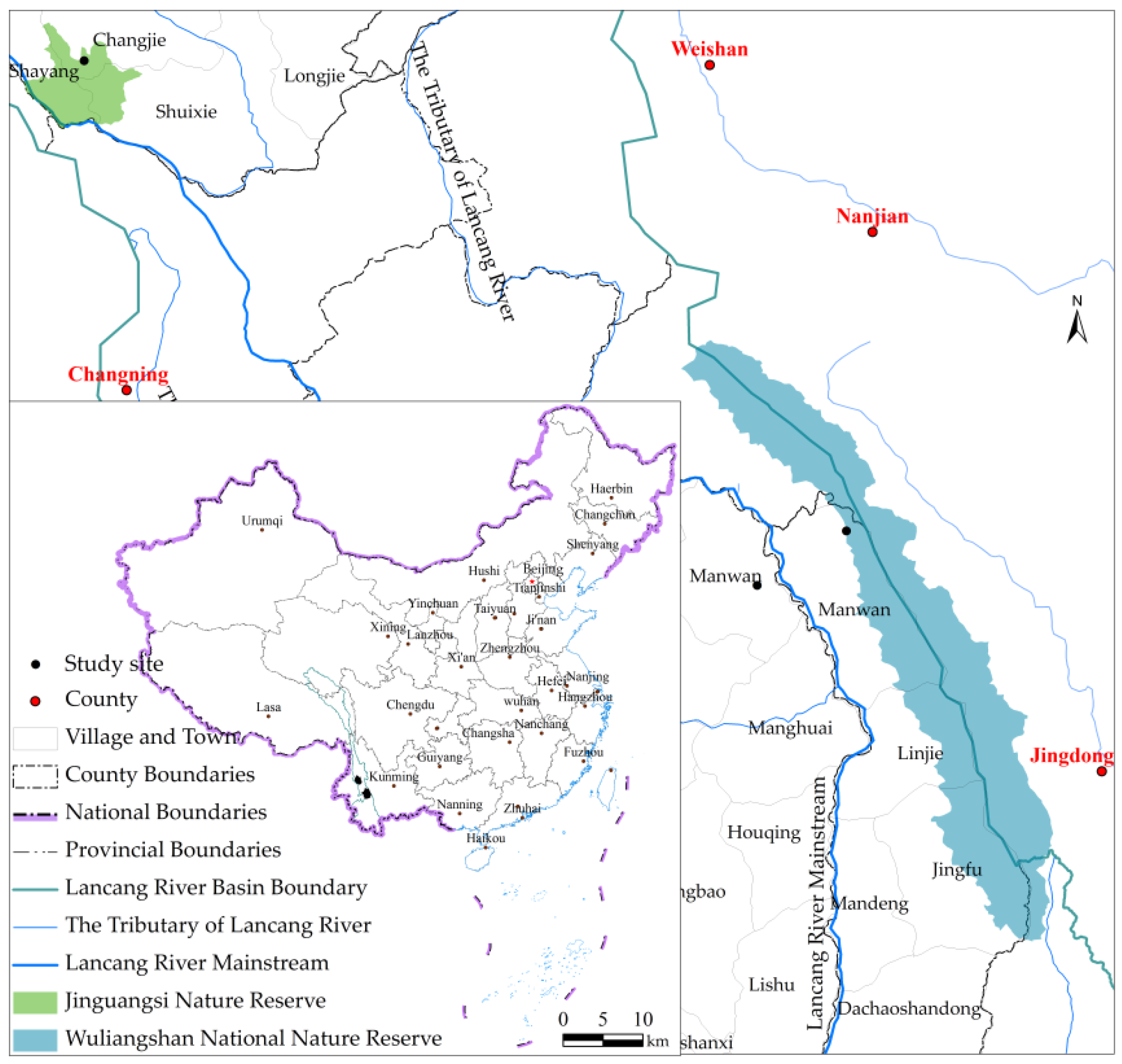
2.1. Study Site

The study was sampled at three sites in a subtropical mountain forest along the lower reach of Lancang River, and the northernmost site was located in the Jinguangsi Nature Reserve (25°7′18″–25°13′44″ N, 99°27′26″–99°36′07″ E) in Yongping County (YP), which is famous for being the best-preserved original semi-humid evergreen broad-leaved forest in Yunnan Province (Figure 1). This nature reserve is typical of mountain landscapes with an altitude ranging from 1150 to 2913 m above sea level. It lies within a mid-subtropical monsoon climate. The annual mean air temperature is about 13 °C, with a mean monthly minimum temperature of 2 °C in January and maximum temperature of 16 °C in June. Mean annual precipitation is 1100–1200 mm. The main soil type is designated as well-drained clay loam mountain red yellow soil developed on slate and shale rock, which is classified as an Alliti-Udic Ferrosol. The vegetation can be divided into semi-evergreen monsoon forest (e.g., Ficus altissima Bl., Bauhinia variegeta Linn.), evergreen broadleaf forest (e.g., Lithocarpus variolosus (Franchet) Chun, Lithocarpus hancei (Benth. ) Rehd.), deciduous broadleaf forest (e.g., Quercus variabils Blume, Alnus nepalensis D. Don), coniferous forest (e.g., Pinus yunnanensis Franch., Pinus armandi Franch.), savanna shrub vegetation (e.g., Woodfordia fruticosa (Linn.) Kurz, Heteropogon contortus (Linn.) P. Beauv. ex Roem. et Schult.), and shrub (e.g., Vaccinium delavayi (Hayata) R. C. Fang, Rhododendron irroratum Franch.) [26].

The second site was Manwan Town (24°37′—24°41′ N, 100°46′—100°32′ E), which stands on the western bank of Lancang River in Yunxian County (YX). Its altitude ranges from 891 to 2834 m above sea level; the mean annual air temperature is about 20 °C, and the average annual precipitation is about 1269 mm. A homonymic town (24°30′—24°44′ N, 100°24′—100°37′ E) is located across the Lancang River in Jingdong County (JD), which was the third site (Figure 1). It is also a typical mountain landscape with an altitude ranging from 885 to 2889 m above sea level, with a mean annual air temperature of about 18 °C, average annual precipitation of about 1087 mm, average annual sunshine time of 2132 h, and average frost-free period of about 355 days. It is located on the western slope of Wuliangshan, covering a 42 km² area in Wuliangshan national nature reserve, which has abundant plant species and communities. The vegetation types from low to high elevation can be divided into the river-valley deciduous monsoon forest, the warm needle-leaved forest (Pinus kesiya Royle ex Gordon var. langbianensis (A.Chev) Gaussen)/monsoon evergreen board-leaved forest (e.g., Castanopsis fleuryi Hickel et A. Camus, Lithocarpus truncates (King ex J. D. Hooker) Rehder et E. H. Wilson, Anneslea fragrans Wall. var. fragrans), the semi-humid evergreen broad-leaved forest (e.g., Castanopsis orthacantha Franch, Schima argentea Pritz. ex Diels, Cyclobalanopsis delavayi (Franchet) Schottky), the mid-mountain humid evergreen broad-leaved forest (e.g., Lithocarpus echinophorus (Hickel et A. Camus) A. Camus, Lithocarpus hancei, Castanopsis wattii (King ex Hook. f.) A. Camus, Lithocarpus xylocarpus (Kurz) Markgraf), and the low mountaintop moss forest (e.g., Rhododendron faceteum Balf. F. et K. Ward, Rhododendron edgeworthii Hook. f., Rhododendron siderophyllum Franch., V. delavayi) [27]. Those two homonymic towns have similar vegetation and similar climate, geographic, and geomorphic conditions. The vegetation in the three study sites is of typical vertical mountain type in mid-subtropical and southern subtropical zones in the LLRB and is as complex as that under natural conditions.

2.2. Field Sampling and Laboratory Methods

To minimize anthropogenic interference at each study site, we established one study strip in natural forest areas in Yunxian County and Jingdong County (March 2010), and Jinguangsi Nature Reserve in Yongping County (August 2011). To exclude the edge effects caused by different types of neighboring forests, we randomly established sample plots within each strip. Forty-five 0.06 ha plots were established in different forests. All individual trees in the plots with diameter at breast height (DBH) ≥5 cm were surveyed. The scientific name, DBH, and height of each tree were recorded during the growing season.

Each plot was characterized by four topographic variables: mean elevation (El), slope degree (Sl), slope aspect (As), and slope position (Po). Mean elevation (m) was the average value of the altitudes of the four corners and the center of each plot, and elevation was estimated by a portable altimeter (Thommen Classic, Switzerland). Slope degree and aspect were measured by a compass and clinometers, respectively. Aspect may be a poor variable for quantitative analysis because 1° is adjacent to 360—the numbers are obviously different, while their aspects are about the same. Thus, the aspect here was transformed to a folded aspect [28]. Slope position was estimated as the bottom, middle, mid-upper part, and top of a slope.

At the four corners and the center of each plot, soil samples were collected randomly from the 0–20 cm depth using a soil corer. If a tree stump or rock occurred at the sampling point, a slightly off-center sampling point was selected when collecting the soil sample. A total of 225 soil samples were collected and transported to the laboratory for the measurements of soil pH and the concentrations of organic matter (OM), total nitrogen (TN), available nitrogen (AN), available phosphorus (AP), and available potassium (AK). After manually removing non-soil materials (e.g., large pieces of plant material, gravel, earthworms), and milling and sieving the soil through a 2-mm mesh, we thoroughly mixed the five selected soil cores from each plot and obtained a representative soil sample for each plot after quartering. Each composite soil sample was stored in an airtight plastic bottle for soil property analysis.

We milled and sieved some of the air-dried soil samples through a 0.149-mm mesh and used the soil for further analysis of OM, TN, AN, AP, and AK. We measured soil OM using potassium dichromate oxidation, TN and AN using the micro diffusion method, AP using the molybdenum blue method, and AK using ammonium acetate extraction-flame photometry. We measured soil pH in water and in a 1.0 M KCl solution using a soil:liquid volume ratio of 1:2, and measured the soil moisture content by means of oven-drying at 105 °C for 24 h. All laboratory procedures followed are outlined in the Analysis Methods of Forest Soil [29].

2.3. Data Analysis

Tree density, mean height, mean DBH, and mean basal area at breast height (BA) were calculated for each tree species, each plot, and each forest type. The dominance (D_i) of each tree in the plot was estimated following the formula: $D_i=\frac{\left(N_i/N+B{A}_i/BA\right)}{2} \times 100$, where N_i is the number of individuals of the i-th tree species in the plot, N is the total number of the individuals in the plot; BA_i is the total basal area at breast height of the individuals of the i-th tree species, and BA is the total basal area at breast height of the individuals of all species in the plot [30].

The four species diversity indices adopted in this paper are Margalef richness (R), which represents the transformed number of species recorded in a plot, the Shannon-Wiener index (H′), the complement of Simpson’s index (D), and Pielou’s evenness index (E) [31,32]. The formulas for the calculation of these indices are outlined in

Table 1. Formulas for calculation of tree species diversity.

Formulas	Note
$R=\left(S-1\right)/\ln N$	S: the number of tree species recorded in the plot; N: the total number of individuals in the plot.
$H^{\prime }=-{\displaystyle \sum }\text{}{P}_i\ln P_i$	Pi: the proportional abundance of the i-th tree species for N individuals of S species in the plot (i.e., $P_i=N_{\mathrm{i}}/N$).
$D=1-{\displaystyle \sum }\text{}{P}_{\mathrm{i}}^2$
$E=H\prime /\ln S$

. We chose these four indices since they have low or moderate sensitivity to plot size and have been widely applied [31].

One-way analysis of variance (ANOVA; with post hoc Tukey’s honestly significant difference test with a probability p ≤ 0.05 or p ≤ 0.01) was used in analyzing the differences in tree structural characteristics, species diversity, and soil variables among study forests or sites, and Pearson’s correlations of environmental variables with forest structure and tree species diversity were calculated. Prior to the ANOVA and Pearson’s correlation analysis, all structural characteristics, species diversity, and soil data were tested for normality with the Shapiro-Wilk W test and for homogeneity of variance with the Levene test, and the non-normal data were log transformed. The statistical software package used here was SPSS, Version 16.0 [33].

To quantify the relationships between tree species abundance and environmental factors, a canonical correspondence analysis (CCA) was employed using the software CANOCO (Version 4.51 for Windows, Microcomputer Power, Ithaca, NY, USA) [34]. In order to perform CCA, we split the data into two distinct matrices: the tree species matrix and the environmental factors matrix. The species matrix consisted of the tree counts per species, per plot. Because rare species have little or no effect on the results of ordination techniques and their elimination reduces the amount of calculations and meaningless results [35], species with relative dominance less than 10% were deleted here, resulting in 59 dominant species in the 46 plot-matrix. The dominance values were transformed by the arcsine (p^1/2) expression prior to the ordination in order to lessen the effects of the few larger values [34]. The environmental factors matrix contained the topographical variables (mean elevation, mean slope degree, aspect, and position) and soil variables (soil pH, OM, TN, AN, AP, and AK). The slope degree was set to range from 1 to 6, being: when Sl were (0°, 8°], (8°, 15°], (15°, 25°], (15°, 25°], (25°, 35°], (35°, 45°] and > 45°, the Sl values were respectively 1, 2, 3, 4, 5 and 6. The slope aspect (in radians) was transformed into two orthogonal variables indicating “northness” (No) and “eastness” (Ea) using SIN(aspect) and COS(aspect), and the slope position was set to range from 1 to 4, being: 1 = bottom slope, 2 = middle slope, 3 = mid-upper slope, and 4 = top slope. All values shown as a percentage were transformed by the arcsine (p^1/2) expression. Elevation and pH were transformed by (X_i − X_mean)/SD (X_mean and SD are the mean and standard deviation of X_i, respectively). After a preliminary CCA analysis, we eliminated four poorly correlated variables, namely No, Ea, AP, and AK. The seven variables remaining in the final CCA were El, Sl, Po, pH, OM, TN, and AN. The correlation significance between matrices was tested with Monte-Carlo permutation with 1000 iterations [36].

3. Results

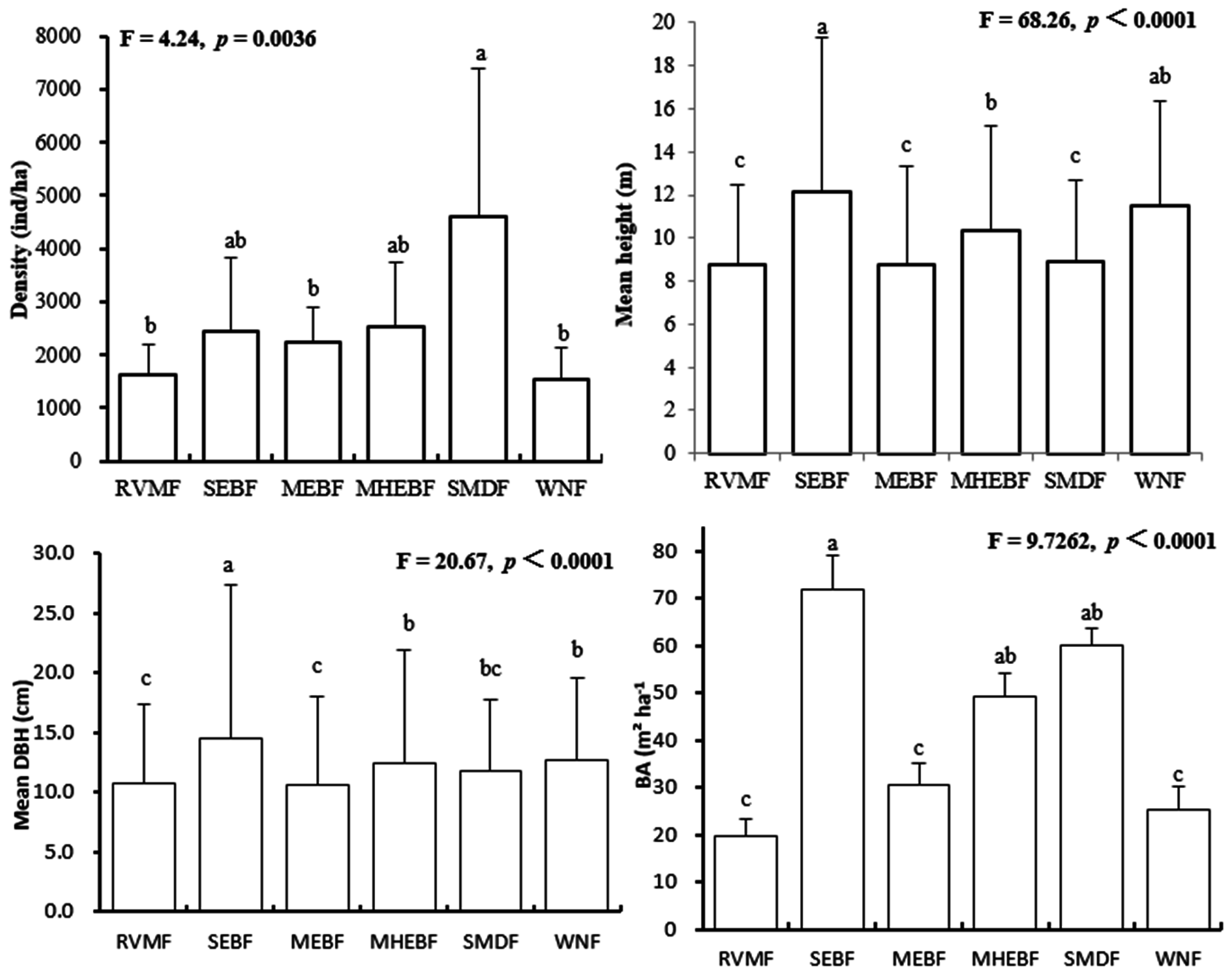
3.1. Forest Structure and Floristic Composition

The vegetation structure of the subtropical mountain forest in the LLRB was demonstrated by forest types of the plots (Table 1). Aspect was not significantly different among forest types (Kruskal-Wallis ANOVA p > 0.05), neither was the soil concentrations of total nitrogen, or available nitrogen and available phosphorus, but for the other measured forest structural characteristics (e.g., topographic, edaphic, and community height), there were marked differences among forest types (

Table 2. Summary statistics of forest plots in six subtropical mountain forests in the LLRB, Yunnan.

Indices	RVMF	SEBF	MEBF	MHEBF	SMDF	WNF
El (m) **	1057 (33.3)c	2414 (98.7)a	1597 (135.3)b	2286 (73.8)a	2396 (155.7)a	1358 (76.1)bc
Sl (°) **	40.8 (2.47)a	28.6 (2.1)ab	30.2 (2.0)ab	30.0 (2.0)a	33.4 (4.2)a	27.3 (2.3)b
As(°) N.S.	130.0 (32.7)	221.9 (25.5)	282.5 (40.2)	233.2 (29.7)	202.0 (45.7)	190.1 (31.6)
pH **	5.9 (0.1)a	4.9 (0.2)b	5.2 (0.1)ab	5.0 (0.1)b	4.7 (0.2)b	5.7 (0.1)a
OM (%) **	2.58 (0.58)b	8.41 (1.51)a	2.14 (0.27)b	7.73 (1.09)a	9.01 (1.80)a	2.16 (0.53)b
TN (g·kg−1) N.S.	3.43 (0.84)	3.71 (0.38)	3.97 (1.16)	10.89 (4.49)	14.59 (4.86)	1.93 (0.38)
AN (mg·kg−1) N.S.	400.49 (219.86)	135.51 (51.72)	248.03 (58.28)	350.26 (109.37)	192.89 (24.36)	41.00 (11.37)
AP (mg·kg−1) N.S.	4.10 (1.10)	4.95 (0.95)	2.44 (0.23)	5.04 (1.53)	6.49 (1.67)	5.36 (1.84)
AK (mg·kg−1) *	20.62 (3.11)b	44.24 (7.68)a	14.47 (3.99)b	28.07 (4.25)ab	28.29 (7.48)ab	25.26 (2.45)ab

The significance levels for ANOVA (parametric or nonparametric) across topographical and edaphic factors are indicated beneath each variable. N.S. = not significant at p = 0.05; * p < 0.05; ** p < 0.01. The values listed in all columns are means and standard errors (SE, in parentheses). Different letters after values indicate significant differences based on t-tests (p < 0.01) among the six forest types.

). Altitude was significantly increased from RVMF to SEBF, and there were no marked differences among SEBF, MHEBF, and SMDF, or among RVMF and WNF, and WNF and MEBF (one-way ANOVA p < 0.01). Slope was lowest in WNF, and no obvious differences existed among other forest types (one-way ANOVA p < 0.01).

Soil pH was not significantly different among SEBF, MEBF, MHEBF, and SMDF, and among RVMF, MEBF, and WNF, while it was markedly highest in RVMF and WNF, and lowest in SEBF, MHEBF, and SMDF (Table 1, Kruskal-Wallis p < 0.01). The soil concentration of available potassium in SENF was obviously higher than that of MEBF and RVMF, and there were no differences among other forest types (Table 2, Kruskal-Wallis p < 0.05).

For all subtropical mountain forests here, the forests had an average basal area of 42.3 (se = 3.8) m²/ha, tree density of 2399 (225) individuals/ha, and mean tree height and mean DBH were 10 (0.1) and 12.1 (0.1) m, respectively. The results of the ANOVAs indicated that tree structural characteristics were significantly different among forest types (Table 2, Kruskal-Wallis p < 0.01). Tree density was obviously higher in SMDF, and there were no differences among the other forests, while mean height, mean DBH, and BA were all significantly highest in SEBF, and lowest in RVMF and MEBF (Figure 2).

We recorded a total of 5155 canopy trees belonging to 204 tree species, 104 genera, and 50 families in 45 plots surveyed across the three sites. Fagaceae, Theaceae, and Lauraceae were the three most diverse families, with 27, 24, and 17 tree species, respectively, and accounted for 33.3% of the tree species identified. The genera Camellia, Castanopsis, Cinnamomum, Cyclobalanopsis, Elaeocarpus, Eurya, Lithocarpus, Rhododendron, Schima, and Symplocos had more species (four or more species each) than those of the other genera.

Table 3. Summary of tree composition in terms of mean basal area at breast height (BA, m²·ha⁻¹) for six studied forests in the LLRB, Yunnan.

Species	Family	Abbreviation	RVMF	SEBF	MEBF	MHEBF	SMDF	WNF
Acer heptalobum Diels	Aceraceae	Ah	-	-	-	0.55	-	-
Acer pubipetiolatum Hu et Cheng	Aceraceae	Ap	-	-	-	0.58	-	-
Albizia odoratissima (Linn. f.) Benth.	Leguminosae	Ao	0.29	-	0.06	-	-	-
Alnus nepalensis	Betulaceae	An	-	0.98	1.08	-	-	-
Ardisia japonica (Thunberg) Blume	Myrsinaceae	Aj	-	0.33	0.73	0.01	-	-
Bauhinia acuminata Linn.	Leguminosae	Ba	3.07	-	-	-	-	-
Bauhinia variegata Linn.	Leguminosae	Bv	2.38	-	-	-	-	-
Castanopsis delavayi Franch.	Fagaceae	Cad	-	5.62	1.95	0.06	-	-
Castanopsis ferox (Roxb.) Spach	Fagaceae	Cfx	-	-	-	0.57	-	-
Castanopsis fleuryi	Fagaceae	Cfi	-	-	1.36	0.20	-	0.03
Castanopsis orthacantha	Fagaceae	Co	-	35.85	-	0.95	-	-
Cinnamomum mollifolium H. W. Li	Lauraceae	Cm	0.04	-	1.18	0.03	-	-
Cipadessa cinerascens (Pell.) Hand.-Mazz.	Meliaceae	Cc	0.84	-	-	-	-	-
Clethra delavayi Franch.	Clethraceae	Cld	-	-	-	-	1.91	-
Cyclobalanopsis delavayi	Fagaceae	Cyd	0.39	-	-	-	-	-
Cyclobalanopsis glaucoides Schotky	Fagaceae	Cg	-	-	0.63	-	-	-
Cyclobalanopsis kontumensis (A. Camus) Y. C. Hsu et H. W. Jen	Fagaceae	Ck	-	-	-	2.24	-	-
Dalbergia obtusifolia (Baker) Prain	Leguminosae	Do	1.37	-	0.09	-	0.06	0.88
Elaeocarpus sylvestris (Lour.) Poir.	Elaeocarpaceae	Els	-	-	-	0.37	-	-
Engelhardia spicata Lesch.	Juglandaceae	Ens	0.5	-	0.23	0.01	-	0.17
Eriolaena kwangsiensis Hand.-Mazz.	Sterculiaceae	Ek	0.34	-	-	-	-	-
Eriolaena spectabilis (DC.) Planchon ex Mast.	Sterculiaceae	Ers	2.39	-	-	-	-	-
Ficus semicordata Buch.-Ham. ex J. E. Smith	Moraceae	Fs	0.37	-	-	-	-	-
Gordonia axillaris (Roxb.) Dietr.	Theaceae	Ga	-	-	-	2.41	0.02	-
Hartia sinensis Dunn	Theaceae	Hs	-	-	-	1.55	0.02	-
Juglans regia Linn.	Juglandaceae	Jr	-	-	0.83	-	-	-
Ilex gingtungensis H. W. Li ex Y. R. Li	Aquifoliaceae	Ig	0.08	-	-	-	2.22	-
Illicium verum Hook. f	Illiciaceae	Iv	-	0.01	-	0.71	-	-
Lannea coromandelica	Anacardiaceae	Lac	0.21	-	-	-	-	-
Lindera communis Hemsl.	Lauraceae	Lic	-	-	0.80	-	-	-
Lithocarpus confinis C. C. Huang ex Y. C. Hsu et H. W. Jen	Fagaceae	Lc	-	-	-	1.42	-	-
Lithocarpus fenestratus (Roxburgh) Rehd. var. brachycarpus A.Camus	Fagaceae	Lf	-	-	0.01	0.11	1.72	-
Lithocarpus glaber (Thunb.) Nakai	Fagaceae	Lg	0.8	4.38	0.89	2.43	2.6	-
Lithocarpus hancei	Fagaceae	Lh	-	-	0.22	1.64	3.03	-
Lithocarpus mairei (Schottky) Rehder	Fagaceae	Lm	-	0.09	-	2.69	1.27	-
Lithocarpus polystachyus	Fagaceae	Lp	-	0.94	-	3.24	-	-
Lithocarpus variolosus	Fagaceae	Lv	0.44	-	4.57	-	-	-
Lyonia ovalifolia (Wall.) Drude	Ericaceae	Lo	-	1.06	0.27	1.74	3.17	0.03
Mallotus yunnanensis Pax et Hoffm.	Euphorbiaceae	My	0.18	-	1.28	-	-	-
Melia azedarach Linn.	Meliaceae	Ma	0.37	-	-	-	-	-
Myrica esculenta Buch.-Ham.	Myricaceae	Me	-	0.17	0.23	0.63	-	-
Neocinnamomum delavayi (Lec.) Liou	Lauraceae	Nd	0.06	-	0.54	1.64	0.03	-
Olea yuennanensis Hand.-Mazz.	Oleaceae	Oy	0.05	-	0.48	0.03	-	-
Phyllanthus emblica Linn.	Euphorbiaceae	Pk	0.55	-	-	-	-	0.14
Pinus kesiya	Pinaceae	Ph	0.18	-	0.34	-	-	21.78
Pinus yunnanensis	Pinaceae	Py	-	6.12	-	0.15	-	-
Quercus acutissima Carr.	Fagaceae	Qa	-	-	2.46	0.83	-	0.01
Quercus kingiana Craib	Fagaceae	Qk	0.45	-	-	-	-	-
Rhododendron delavayi	Ericaceae	Rd	-	3.33	-	1.43	16.98	-
Rhododendron simsii Planch.	Ericaceae	Rs	-	-	-	0.16	16.78	-
Schima argentea	Theaceae	Sa	-	-	1.41	2.75	0.15	0.02
Schima khasiana Dyer	Theaceae	Sk	-	-	0.94	-	-	-
Schima noronhae Reinw. ex Bl. Bijdr.	Theaceae	Sn	-	-	0.95	-	-	0.13
Schima superba Gardn. et Champ.	Theaceae	Ss	<0.01	3.79	0.75	1.11	1.21	0.73
Symplocos hookeri Clarke	Symplocaceae	Sh	0.26	-	-	-	-	-
Toona ciliata Roem.	Meliaceae	Tc	0.32	-	-	-	-	-
Vaccinium bracteatum Thunb.	Ericaceae	Vb	-	0.87	0.18	2.26	0.3	-
Vaccinium duclouxii	Ericaceae	Wd	-	0.77	0.55	5.19	0.01	0.02
Wendlandia scabra Kurz	Rubiaceae	Ws	0.71	0.02	-	-	-	0.03
The others 145	-	-	3.11	7.37	4.91	9.57	6.32	1.29

lists the 59 (out of 204) most dominant tree species recorded in the total sample with average BA and D_i for mountain forests. In subtropical mountain forests in the LLRB, Yunnan, the dominant family in these 59 most dominant species (relative density or relative basal area ≥10) was the Fagaceae (16 tree species), the second (6 species) was the Theaceae, the third (5 species) was the Ericaceae, and they varied with forest type. The dominant genus in those 59 most dominant species was Lithocarpus (7 species), the second was Castanopsis and Schima (each had 4 species), and the third was Cyclobalanopsis (3 species), and they also varied with forest type. For SEBF, SMDF, and WNF, the value of BA for the first dominant tree was significantly higher than that of the second. C. orthacantha, Rhododendron delavayi Franch., and P. kesiya were their main dominant trees, which contributed 50.0%, 30.7%, and 75.8% of their forest tree BA, respectively. On the contrary, the main dominant tree was less obvious for RVMF, MEBF, and MHEBF; their main dominant trees, Bauhinia acuminate Linn., L. variolosus, and Vaccinium duclouxii (Levl.) Hand.-Mazz., only had values of 3.07, 4.57, and 5.19 m²·ha⁻¹, respectively, which were about 15.6%, 15.3%, and 10.5% of their respective forest tree BA values.

3.2. Tree Species Diversity

Table 4. Richness and diversity of six subtropical mountain forests and study sites in the LLRB, Yunnan.

Indexes	Forest Types **						Study Sites N.S.
	RVMF	SEBF	MEBF	MHEBF	SMDF	WNF	YP	YX	JD
S	14.0 (1.2)ab	11.4 (1.3)abc	18.0 (1.4)a	16.0 (1.0)ab	10.0 (1.5)bc	6.4 (1.2)c	11.8 (1.2)	12.9 (1.3)	13.3 (1.3)
R	2.89 (0.22)ab	2.30 (0.28)abc	3.56 (0.32)a	3.15 (0.21)a	1.77 (0.30)bc	1.22 (0.23)c	2.40 (0.23)	2.49 (0.24)	2.63 (0.29)
H	2.13 (0.12)a	1.83 (0.14)a	2.30 (0.12)a	2.10 (0.10)a	1.35 (0.24)ab	0.85 (0.24)b	1.90 (0.12)	1.71 (0.15)	1.79 (0.19)
D	0.83 (0.02)a	0.77 (0.04)a	0.85 (0.02)a	0.81 (0.02)a	0.57 (0.09)ab	0.37 (0.11)b	0.68 (0.07)	0.79 (0.03)	0.69 (0.05)
E	0.81 (0.02)a	0.75 (0.04)a	0.80 (0.03)a	0.77 (0.03)a	0.58 (0.07)ab	0.43 (0.09)b	0.78 (0.03)	0.67 (0.04)	0.70 (0.03)

The significance level for ANOVA (parametric or nonparametric) is indicated. N.S. = not significant at p = 0.05; ** p < 0.01. S, the number of tree species recorded in the plot; R, Margalef richness; H′ the Shannon-Wiener index; D, the complement of Simpson’s index; and E, Pielou’s evenness index. Different letters after values indicate significant differences based on t-tests (p < 0.01) among the six forest types.

shows the species diversities of tree populations in these six mountain forest types and three sites. Overall, the tree species diversities per plot are not statistically significant between sites (p > 0.05), while there are significant differences between the species diversities of different forest types (p < 0.01, Table 4). The tree species diversity per plot of the total sample, measured by the number of species, Margalef richness, Shannon-Wiener diversity, Simpson’s index, and Pielou’s evenness was 12.8, 2.53, 1.78, 0.71, and 0.70, respectively. Although the differences in species diversities is not statistically significant between sites, based on a comparison with subtropical mountain forests in YP and YX, JD mountain forests display a slightly higher number of species and Margalef richness, and YP forests display slightly higher Shannon-Wiener diversity and Pielou’s evenness values.

The Margalef richness and Shannon-Weiner diversity indices of the six mountain forests were significantly different, with a lower value for WNF, which was also associated with lower Pielou’s evenness (0.43) that reflected large tree species dominance in WNF. Therefore, the highest species diversity occurred in MEBF, the lowest species diversity occurred in WNF, and the differences were not significant between SMDF and WNF, and the others forest types (p > 0.01, Table 4). The greatest similarity in dominant tree species composition among the forest types was observed between MEBF and MHEBF; they shared 13 of the most abundant tree species, such as A. japonica, Castanopsis delavayi, C. fleuryi, L. glaber, L. hancei, L., N. delavayi, Q. acutissima, S. argentea, S. superba, V. bracteatum, and V. duclouxii, and RVMF was the least similar to those two in terms of tree species composition (Table 3).

3.3. Relationships among Environmental Factors, Forest Structure, and Tree Species Diversity Indices

Stand structure and tree species diversity were strongly related to topographical and edaphic factors in the Pearson’s correlation analysis. The mean tree height, DBH, and BA of forests were positively correlated with elevation and negatively correlated with soil pH, and tree species diversity indices were positively associated with AN, and S and R were also closely associated with AP. AN, AP, and AK were significantly associated with mean tree height; Po, pH, and AK were significantly correlated with mean DBH and BA; and pH and OM were closely associated with the mean tree density of the stand (

Table 5. Correlation coefficients between environmental variables and stand structure and tree diversity.

	Mean height	DBH	Tree density	Mean BA	S	R	H	D	E
El	0.3002 *	0.4285 **	0.2745	0.7098 **	−0.0003	−0.0117	0.0582	0.1258	0.1071
Sl	−0.1309	−0.1048	0.0901	−0.0481	0.1814	0.1638	0.2307	0.2150	0.2168
Po	−0.2733	−0.3114 *	−0.1657	−0.4250 **	0.1703	0.2011	0.0954	0.0478	0.0381
No	0.0451	0.0664	−0.0239	−0.0077	−0.1409	−0.1386	−0.0604	0.0155	0. 0103
Ea	−0.0736	−0.1242	−0.0008	0.0015	0.1669	0.1606	0.1401	0.0946	0.1018
pH	−0.3065 *	−0.3420 *	−0.3277 *	−0.6497 **	−0.1453	−0.1128	−0.1879	−0.2089	−0.2021
OM	0.0624	0.2926	0.3120*	0.5710 **	0.0941	0.0558	0.1307	0.2068	0.1760
TN	0.0997	−0.0136	0.2524	0.2112	0.2952 *	0.2768	0.2198	0.1675	0.1468
AN	−0.3182 *	−0.0736	−0.0298	−0.0215	0.4562 **	0.4265 **	0.3947 **	0.3839 **	0.3335 *
AP	0.4094 **	0.2745	−0.0704	0.0775	−0.3472 *	−0.3059 *	−0.2420	−0.2384	−0.1737
AK	0.5362 **	0.4050 **	−0.0375	0.3108 *	−0.0859	0.0135	0.1234	0.1460	0.2313

* p < 0.05; ** p < 0.01.

).

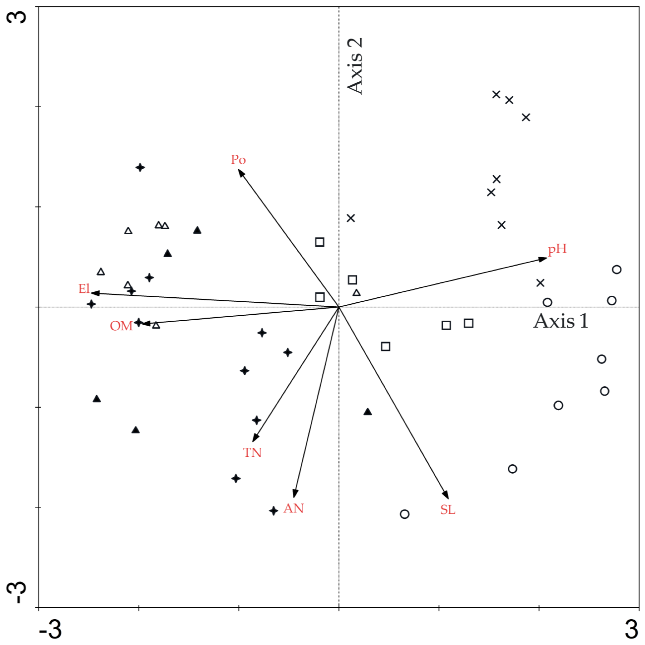
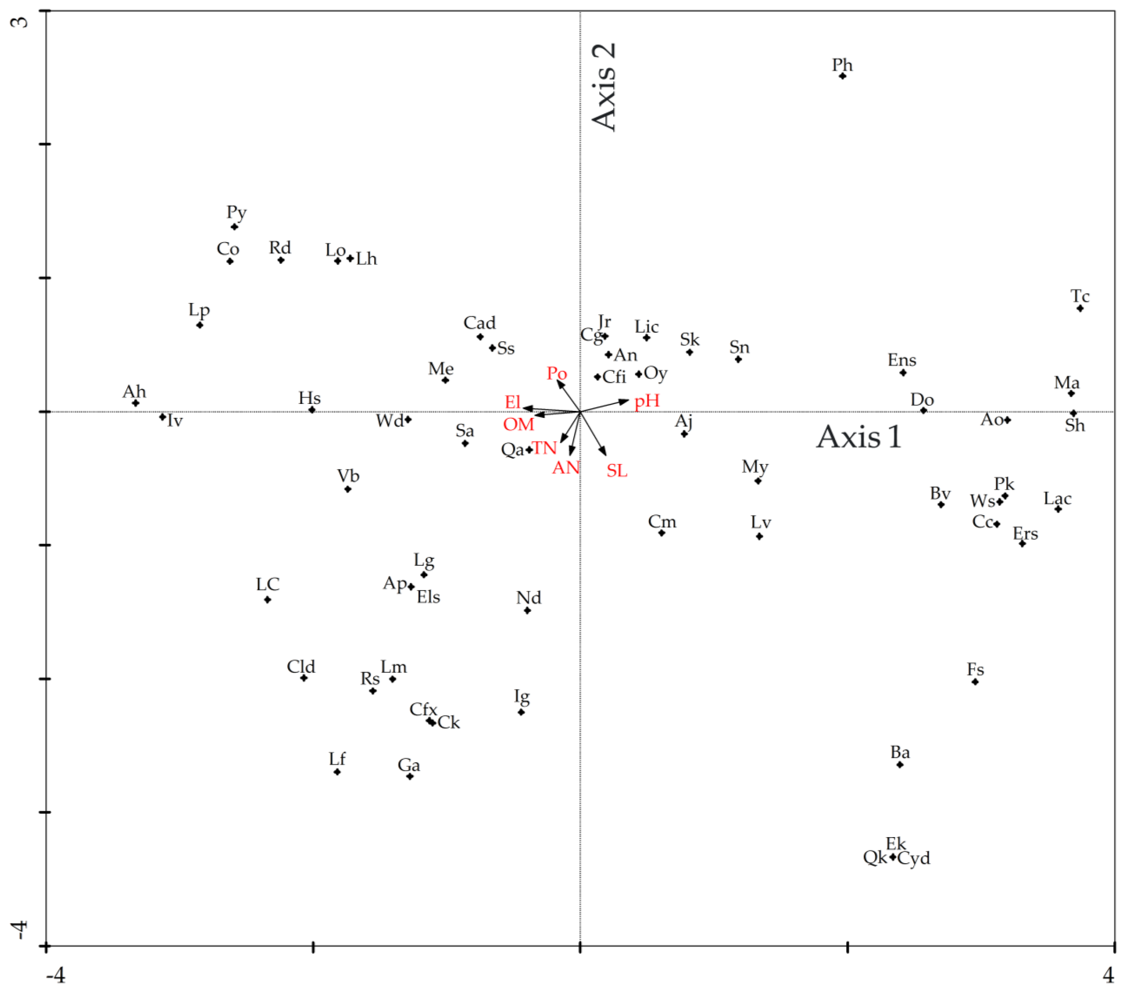
3.4. Direct Gradient Ordination Analysis

The CCA was carried out for 45 plots and dominant trees (59 species) with seven explanatory variables. For dominant trees here, the eigenvalues obtained for the first and second axes were 0.742 and 0.485, respectively. The species-environment correlations coefficients were 0.957 for axis1 and 0.872 for axis2. The cumulative percentage of variance explained by the first four axes accounted for 19.0% of the species data variation and 74.6% of the species-environment variation. The Monte-Carlo test indicated that all ordination axes were marked (p < 0.01) (

Table 6. Eigenvalues and cumulative percentage variance of canonical correspondence analysis (CCA) ordination.

Axes	1	2	3	4
Eigenvalues	0.774	0.485	0.404	0.331
Species-environment correlations	0.957	0.872	0.833	0.857
Cumulative variance of species	7.2	11.9	15.8	19.0
Cumulative variance of species-environment relation	28.2	46.7	62.0	74.6

).

The first axis was significantly positively correlated with the slope and soil pH (p < 0.01), markedly negatively correlated with elevation, slope position, and OM (p < 0.01), and obviously negatively correlated with TN (p < 0.05). The second axis was positively associated with slope position, TN, and AN (p < 0.01), and negatively correlated with slope degree (p < 0.01). The third axis was associated with position, TN, and AN. The fourth axis was correlated with TN and AN (p < 0.01), and significantly positively correlated with OM (Table 6). Significant correlations were found between topographic and soil factors. Elevation was significantly correlated with soil pH, OM, and total N (p < 0.01), and slope position was obviously correlated with soil available N (p < 0.05) (

Table 7. Correlation coefficients between CCA axes and environmental variables, and soil and topographical variables.

Factors	Axis 1	Axis 2	Axis 3	Axis 4	Sl	Po	pH	OM	TN	AN
El	−0.9334 **	0.0427	0.0669	0.1393	−0.4227 **	0.4877 **	−0.7786 **	0.7639 **	0.4266 **	0.0204
Sl	0.4127 **	−0.5769 **	−0.1549	0.0795	-	−0.4662 **	0.1610	−0.2045	0.0204	0.2160
Po	−0.3789 **	0.4155 **	0.5545 **	−0.0442		-	−0.2054	0.0721	0.1721	−0.3387 **
pH	0.7844 **	0.1484	−0.0861	0.0433			-	−0.6502 **	−0.4275 **	−0.1628
OM	−0.7416 **	−0.0507	−0.2292	0.3278 *				-	0.3574 *	0.2427
TN	−0.3249 *	0.4050 **	0.4621 **	0.4805 **					-	0.0326
AN	−0.1692	0.5729 **	−0.1447	−0.4317 **						-

* p < 0.05, ** p < 0.01.

).

As shown in the CCA ordination diagram based on the first two axes, all of the forest communities generated by the vegetation classification system proposed by Wu et al. [21] had their own distribution ranges and limits (Figure 3). RVMF was distinct for the lowest elevation and OM, bottom slope, higher pH, a greater slope degree, and poor soil fertility and contained mostly light-demanding and drought-tolerant species such as B. acuminata, E. spectabilis, B. variegata, D. obtusifolia, C. cinerascens, and L. glaber. WNF was mainly distributed in the low elevation, middle slope habitats, with low slope degree and poor soil fertility. With the elevation increasing, MEBF occurred and were located at medium elevation with moderate soil fertility and slope degree. SEBF, SMDF, and MHEBF seemed to have a similar distribution gradient; they were distributed across higher elevations with lower pH and rich soil fertility and were comprised of shade-tolerant species like C. orthacantha, V. duclouxii, L. glaber, and R. delavayi, etc.

Figure 4 reveals that Acer heptalobum, Illicium verum, Myrica esculenta, Schima argentea, Wendlandia scabra, Hartia sinensis, A. japonica, Albizia odoratissima, Dalbergia obtusifolia, Melia azedarach, and Symplocos hookeri are closely associated with elevation and soil OM in both directions, whereas Lithocarpus fenestratus, Gordonia axillaris, Castanopsis ferox, Cyclobalanopsis kontumensis, Cyclobalanopsis delavayi, Eriolaena kwangsiensis, and Quercus kingiana did not show significant associations with these factors. On the other hand, E. kwangsiensis, Q. kingiana, Cyclobalanopsis delavayi, Cinnamomum mollifolium, Castanopsi delavayi, and S. superba are highly associated with slope degree and slope position, whereas Toona ciliata, M. azedarach, S. hookeri, Engelhardia spicata, and Vaccinium bracteatum are unaffected by these factors, but they are associated closely with the soil pH value. Further, on the left hand side of this figure, soil TN shows a clear association with a number of tree species such as Lindera communis, Olea yuennanensis, Elaeocarpus sylvestris, L. mairei, and Rhododendron simsii, whereas, C. fleuryi, Alnus nepalensis, C. glaucoides, Neocinnamomum delavayi, and Ilex gingtungensis are associated closely with soil AN.

4. Discussion

4.1. Variation in Stand Structure and Tree Diversity among Forests

Both forest structure and tree diversity varied across the subtropical mountain forest in the LLRB. The subtropical mountain forest investigated in 45 plots in this study had 5155 stems (DBH ≥ 5 cm) from 204 species of 104 genera and 50 families, which supports reports that subtropical mountain forests contain a higher diversity of tree species [37,38,39]. The warm needle-leaved forest contained a significant lower diversity of tree species and lower Pielou’s evenness in the LLRB, which was consistent with a previous suggestion by Wang et al. (i.e., that its species parabolic low and species richness are extremely low) [23]. Previous studies have demonstrated that there were no significant differences in tree species diversities, viz. S, H’, D, and E, between WNF and MEBF in Xishuangbanna, while their values of tree species number were significantly higher than those of the WNF [23]. By contrast, Peng and Wu found that the tree species composition of SEBF was obviously lower than MHEBF in Wuliangshan National Nature Reserve [40]; similar conclusions were reported by Tian et al. for Wuliang Mountain [41] and Wang et al. for Gaoligong mountains [42]. Tang suggested that the MEBF yielded the highest indices of H’, E, D, and Fisher’s alpha, followed by the mid-montane moist evergreen broad-leaved forest, and the semi-humid forest for Yunnan subtropical montane evergreen broad-leaved forests [43]. However, Cao et al. found that there were no significant differences in tree species number among RVMF, MEBF, and WNF in the Nuozhadu nature reserve [44].

The above studies indicate that the results varied with different study objectives or study sites. Our study showed that MEBF yielded the highest tree diversity indices of S, R, H’, D, and E, followed by MHEF, then by RVMF and SEBF, and were lowest in WNF, while no significant differences in tree diversity indices were found among MEBF, MHEF, RVMF, and SEBF. Therefore, in view of the differences in the flora of subtropical mountain forests, our results were good compared with the previous reports for the Lancang’s lower reaches and its adjacent area.

4.2. Topographical and Edaphic Impact on Forest Structure and Tree Diversity Indices

Forest structure and tree diversity were strongly related to topography and soil properties in the Pearson’s correlation analysis. The elevation was the foremost topographical factor influencing stand structure of the subtropical mountain forest in the LLRB, followed by slope position. Elevation was significantly associated with the mean height, DBH, and BA, and Po was negatively correlated with DBH and BA, while forest structure was not related to Sl, No, and Ea (Table 5). For elevation, Wilcke et al. found that forest stature, tree basal area, and tree height decreased significantly with elevation in Ecuadorian tropical mountain forest, and the concentrations of all nutrients except Ca in the A horizons correlated significantly negatively with altitude [45]. By contrast, Zheng et al. reported that the largest maximum tree height and maximum DBH were found at middle elevations, but not at upper or lower elevations for subtropical evergreen broad-leaved forests in Wuyi Mountains, Fujian, China [46]. As for the relationship between elevation and tree diversity, some previous studies showed that S and H’ were markedly negatively correlated with elevation [46,47]. On the contrary, Xian found these two parameters were significantly positively associated with elevation [48], while Wang et al. reported that the tree species richness increased rapidly first and then decreased with increasing elevation, peaking at about 1600 m for mountain forest in Gaoligong Mountains near our study site [49]. Therefore, the relationships between elevation and stand structure and tree species diversity might be complex. Other authors reported contrasting results on the elevation-stand structure/tree diversity relationship, which may have several reasons, such as differences in research objects, study site, and forest succession stage.

As for the relationship between stand structure and soil properties, we found significant correlations between tree height, DBH, tree density, and BA, and several parameters characterized the soil properties. The closest correlation with stand structure was found for soil pH and AK; the tree height, DBH, and BA were all influenced by soil pH and AK, and soil pH also influenced the tree density. In contrast, the nutrient concentrations of soil OM, AN, and AP were found to be much less influential, and soil TN had no influence (Table 5). The dominant role of soil properties matches previous findings, for instance, Tateno and Takeda found that soil pH was significantly associated with tree density, mean height, and mean DBH [49], and Xu et al. also found a role of pH as a prominent soil property influencing forest structure [50]. For soil nutrients, Unger revealed that BA and DBH varied primarily with AK [51], and Vitousek reported the role of AP as a prominent soil nutrient influencing stand structure [52]. However, in contrast to our results, Xu et al. found no stronger correlation between soil nutrients and stand structure (BA, tree density, mean DBH, and mean height) in an Okinawan subtropical forest [50]. Other authors reported contrasting results on the soil property-stand structure correlation, which may have several reasons, among them the regional contrasts in the spatial variability of soil fertility in the study region, different methods applied by the authors in characterizing soil nutrient availability, or different experimental subjects under different human-caused disturbance and different climate zones.

In regards to the relationship between soil property and tree species diversity, significant correlations were found between soil nutrient and tree diversity here. AN was markedly associated with all tree species diversity indices, and significant correlations were found between TN and S, AP and S, and AP and R, therefore AN plays a role as a prominent soil property influencing tree diversity in subtropical mountain forests in the LLRB. Our results contrast with the previous findings in, or nearby, the LLRB; for example, Xu et al. found that total K was the prominent soil factor influencing tree diversity in Xishuangbanna tropical seasonal rainforests, while the AP influence was not significant [17]. Xu et al. reported that AK was one of the prominent soil chemical properties influencing tree diversity in an Okinawan subtropical forest, and also found that tree diversity was obviously correlated with AP, OM, and TN, but not with soil pH [50]. Further, Xian revealed that soil pH, OM, TN, AN, and AK were significantly associated with S and H’, OM and TN were also related to E, and AK correlated with D, while the AP influence was not significant for vegetation on the eastern slope of Gaoligong Mountains [48]. Therefore, the relationships between soil properties and tree species may be very complex and may be influenced by study site, dominant community, elevation gradient, and climatic type.

4.3. Topographical and Edaphic Impact on Tree Species Distribution

We found that the most important environmental factor determining the distribution of tree community was elevation, as found previously in the middle-low reach of Lancang-Mekong River [4,15,53,54]. Previous studies have also shown that tree species are more sensitive to elevation than soil fertility or nutrient levels [2,55,56]. Elevation is also known to decrease soil acidity and increase OM and TN [48,52,57]. Thus nitrogen-fixing woody plants, especially Bauhinia acuminata and B. variegata, were only found in RVMF, which was distinct for having the lowest elevation, higher pH, and poor soil fertility, and some woody legumes, such as A. odoratissima and D. obtusifolia, had higher BA in RVMF than other forests.

The other topographic factors, such as Po and Sl, seemed to be related to tree species distribution, as found previously [58,59]. Shade-tolerant trees, such as Bauhinia acuminata, Ficus semicordata, and L. variolosus [23] grew in the valley with a high slope degree, and intolerant tree species, such as C. orthacantha, Pinus yunnanensis, and Rhododendron delavayi often formed abundant patches in the upper slope with gentle incline, just as Yu et al. found in Wuliangshan National nature reserve [60].

Soil pH and OM were the second most important environmental factors associated with the distribution of vegetation in subtropical mountain forests, as found previously [61,62,63]. Acid trees, such as V. bracteatum, L. confinis, and H. sinensis [20] formed abundant patches in plots with a low pH value and high OM value, and acidulous trees, such as M. azedarach, S. hookeri, and Toona ciliata were found in RVMF with a high dominance value and a low OM value.

Soil TN and AN were other important soil nutrient factors controlling the distribution of dominant tree species [64,65]. The ordination analyses emphasized that TN and AN have an impact on the distribution of dominant tree species in subtropical mountain forests in the LLRB. Therefore, our result was similar to the previous reports in the LLRB [14]. However, Zhang et al. found TN and AN were not significantly correlated to any of the first three species axes for subtropical Karst forests on top of the mountain [2], and this difference could be ascribed to the differences in physiognomy, climate, and plant species.

The cumulative percentage of variance explained by the first four axes accounted for 19.0% of the species data variation and 74.6% of the species-environment variation here, so at a stand scale, topographic and soil factors are the important drivers determining the distribution of the dominant tree species in subtropical mountain forests of the LLRB, and the topographical factors were more important than edaphic factors in this study. Understanding the relative importance of the local environmental factors determining tree community compositions can improve the efficiency of future vegetation restoration and biodiversity protection measures [2,66]. Results from this study suggested that tree species used in vegetation construction and stand conversion should be carefully selected according to local environmental characteristics in complex subtropical mountainous vertical climatic zones in the LLRB. For example, the light-demanding and drought-tolerant species B. acuminata, B. variegata, D. obtusifolia, E. spectabilis, and P. kesiya should be planted or restored mainly on lower slopes, while R. delavayi, R. simsii, L. hancei, L. ovalifolia, L. mairei, and Cyclobalanopsis delavayi are better selections for the upper and middle slopes.

5. Conclusions

The results from this present study indicated that tree species diversity was higher in forest communities at higher elevation and with lower pH and higher TN and AN; stand structure and tree species distribution were significantly influenced by topographical and soil variables, and elevation was the most important environmental factor in determining tree structure and tree species distribution of subtropical mountain forests in the lower reach of Lancang River, while AN was the most important environmental factor influencing tree species diversities. Except for topographical and edaphic variables, tree physiological characteristics, such as shade-tolerance, acid-tolerance, and reproductive strategy of the tree species, may have more influence than environmental factors. This information concerning tree species distribution in subtropical mountain forests of the LLRB could help decision-makers to design appropriate strategies for vegetation restoration and forest management. In practice, tree species selection for mixed plantation establishment and tree species structural adjustment of low yielding forests, planting site selection for main indigenous tree species, and selective cutting for artificially promoted regeneration are essential for forest management and biodiversity protection.

References

1. Liu, J.; Tan, Y.; Slik, J.W.F. Topography related habitat associations of tree species traits, composition and diversity in a Chinese tropical forest. For. Ecol. Manag. 2014, 330, 75–81. [Google Scholar] [CrossRef]
2. Zhang, Z.; Hu, G.; Ni, J. Effects of topographical and edaphic factors on the distribution of plant communities in two subtropical karst forests, Southwestern China. J. Mt. Sci. 2013, 10, 95–104. [Google Scholar] [CrossRef]
3. Jia, H.R.; Chen, Y.; Yuan, Z.L.; Ye, Y.Z.; Huang, Q.C. Effects of environmental and spatial heterogeneity on tree community assembly in Baotianman National Nature Reserve, Henan, China. Pol. J. Ecol. 2015, 63, 175–183. [Google Scholar] [CrossRef]
4. Liu, Y.; Zhang, Y.; He, D.; Cao, M.; Zhu, H. Climatic control of plant species richness along elevation gradients in the Longitudinal Range-Gorge Region. Chin. Sci. Bull. 2007, 52, 50–58. [Google Scholar] [CrossRef]
5. Barni, E.; Bacaro, G.; Falzoi, S.; Spanna, F.; Siniscalco, C. Establishing climatic constraints shaping the distribution of alien plant species along the elevation gradient in the Alps. Plant Ecol. 2012, 213, 757–767. [Google Scholar] [CrossRef]
6. Woodward, F.I.; Williams, B.G. Climate and plant distribution at global and local scales. Vegetatio 1987, 69, 189–197. [Google Scholar] [CrossRef]
7. Katabuchi, M.; Kurokawa, H.; Davies, S.J.; Tan, S.; Nakashizuka, T. Soil resource availability shapes community trait structure in a species-rich dipterocarp forest. J. Ecol. 2012, 100, 643–651. [Google Scholar] [CrossRef]
8. Baldeck, C.A.; Harms, K.E.; Yavitt, J.B.; John, R.; Turner, B.L.; Valencia, R.; Navarrete, H.; Davies, S.J.; Chuyong, G.B.; Kenfack, D.; et al. Soil resources and topography shape local tree community structure in tropical forests. Proc. R. Soc. B Biol. Sci. 2013, 280, 323–326. [Google Scholar] [CrossRef] [PubMed]
9. Laurance, S.G.W.; Laurance, W.F.; Andrade, A.; Fearnside, P.M.; Harms, K.E.; Vicentini, A.; Luizão, R.C.C. Influence of soils and topography on Amazonian tree diversityA landscape-scale study. J. Veg. Sci. 2010, 21, 96–106. [Google Scholar] [CrossRef]
10. Odgaard, M.; Bøcher, P.; Dalgaard, T.; Moeslund, J.; Svenning, J.C. Human-driven topographic effects on the distribution of forest in a flat, lowland agricultural region. J. Geogr. Sci. 2014, 24, 76–92. [Google Scholar] [CrossRef]
11. Fadrique, B.; Homeier, J. Elevation and topography influence community structure, biomass and host tree interactions of lianas in tropical montane forests of southern Ecuador. J. Veg. Sci. 2016, 27, 958–968. [Google Scholar] [CrossRef]
12. Toledo, M.; Peña-Claros, M.; Bongers, F.; Alarcón, A.; Balcázar, J.; Chuviña, J.; Leaño, C.; Licona, J.C.; Poorter, L. Distribution patterns of tropical woody species in response to climatic and edaphic gradients. J. Ecol. 2012, 100, 253–263. [Google Scholar] [CrossRef]
13. Xiu, Y.; Ma, K.M.; Wang, D. Partitioning the effects of environmental and spatial heterogeneity on distribution of plant diversity in the Yellow River Estuary. Sci. China Life Sci. 2012, 55, 542–550. [Google Scholar]
14. Li, J.; Dong, S.; Yang, Z.; Peng, M.; Liu, S.; Li, X. Effects of cascade hydropower dams on the structure and distribution of riparian and upland vegetation along the middle-lower Lancang-Mekong River. For. Ecol. Manag. 2012, 284, 251–259. [Google Scholar] [CrossRef]
15. Li, J.; Dong, S.; Peng, M.; Li, X.; Liu, S. Vegetation distribution pattern in the dam areas along middle-low reach of Lancang-Mekong River in Yunnan Province, China. Front. Earth Sci. 2012, 6, 283–290. [Google Scholar] [CrossRef]
16. Zhu, H.; Wang, H.; Li, B. Plant diversity and physiognomy of a tropical montane rain forest in Mengsong, southern Yunnan, China. Acta Phytoecol. Sin. 2004, 28, 351–360. [Google Scholar]
17. Xu, W.; Song, C.; Li, Q. Relationship between soil resource heterogeneity and tree diversity in Xishuangbanna Tropical Seasonal Rainforest, Southwest China. Acta Ecol. Sin. 2015, 35, 7756–7762. [Google Scholar]
18. Department of Biology, Yunnan University. An abstract of the survey of plant communities for the establishment of the nature conservation stations in the tropical and subtropical regions of Yunnan Province, China. J. Yunnan Univ. Nat. Sci. 1960, 3, 1–166. [Google Scholar]
19. Survey Croup of Xishuangbanna Nature Reserve. Reports on A Comprehensive Survey of the Xishuangbanna Nature Reserve; Yunnan Science and technology Press: Kunming, China, 1987. [Google Scholar]
20. Integrated survey of west line project of waters transfer from south to north in China, Chinese Academy of Sciences. In Forest in Western Sichuan and Northern Yunnan in China; Science Press: Beijing, China, 1966.
21. Wu, Z.; Zhu, Y.; Jiang, H. The Vegetation of Yunnan; Science Press: Beijing, China, 1987. [Google Scholar]
22. Lü, X.; Yin, J.; Tang, J. Structure, tree species diversity and composition of tropical seasonal rainforests in Xishuangbanna, south-west China. J. Trop. For. Sci. 2010, 22, 260–270. [Google Scholar]
23. Wang, Z.; Xiong, Y.; Huang, J.; Yang, S.; Li, H.; Yang, H. Xishuangbanna National Nature Reserve; Yunnan Education Press: Kunming, China, 2006. [Google Scholar]
24. Wang, J.; Du, F.; Yang, Y.; Tian, K.; Wang, Y. Scientific Investigation and Research of Lancangjiang Nature Reserve; Science Press: Beijing, China, 2010. [Google Scholar]
25. Li, H.; Jiangcunxiluo; Li, H.; Xiao, L.; Li, C.; Fan, Z.; He, X.; Shen, Y.; Zhong, T.; Zhang, H. Baimaxueshan National Nature Reserve; The Nationalitiies Publishing House of Yunnan: Kunming, China, 2003. [Google Scholar]
26. Zhang, Y.; Shi, H. Status of Jinguangsi nature reserve and the countermeasures for development. For. Invent. Plan. 2007, 32, 76–78. [Google Scholar]
27. Peng, H. The endemism in the flora of seed plants in MT. Wuliangshan. Acta Bot. Yunnan 1997, 19, 1–14. [Google Scholar]
28. Mccune, B.; Keon, D. Equations for potential annual direct incident radiation and heat load. J. Veg. Sci. 2002, 13, 603–606. [Google Scholar] [CrossRef]
29. State Forestry Administration of China. LY/T 1210~1275—1999 Foresty Industry Standards of China: Analysis Methods of Forest Soil; Standards Press of China: Beijing, China, 1999.
30. Cao, M.; Zhang, J.H. Tree species diversity of tropical forest vegetation in Xishuangbanna, SW China. Biodivers. Conserv. 1997, 6, 995–1006. [Google Scholar] [CrossRef]
31. Magurran, A.E. Ecological Diversity and Its Measurement; Princeton University Press: Princeton, NJ, USA, 1988. [Google Scholar]
32. Shannon, C.E. A mathematical theory of communication. In The Mathematical Theory of Communication; Shannon, C., Weaver, W., Eds.; University of Illinois Press: Urbana, IL, USA, 1949; pp. 29–125. [Google Scholar]
33. Zhou, Y.; Deng, W. SPSS16.0 and Statistical Data Analysis; Southwestern University of Finance and Economics Press: Chengdu, China, 2002. [Google Scholar]
34. LepŠ, J.; Šmilauer, P. Multivariate Analysis of Ecological Data Using CANOCO; Cambridge University Press: New York, NY, USA, 2003. [Google Scholar]
35. Causton, D.R. An Introduction to Vegetation Analysis, Principles, Practice and Interpretation; Unwin Hyman: London, UK, 1988. [Google Scholar]
36. Ter Braak, C.J. The analysis of vegetation-environment relationships by canonical correspondence analysis. Vegetatio 1987, 69, 69–77. [Google Scholar] [CrossRef]
37. Li, L.; Huang, Z.; Ye, W.; Cao, H.; Wei, S.; Wang, Z.; Lian, J.; Sun, I.F.; Ma, K.; He, F. Spatial distributions of tree species in a subtropical forest of China. Oikos 2009, 118, 495–502. [Google Scholar] [CrossRef]
38. Bruelheide, H.; Böhnke, M.; Both, S.; Fang, T.; Assmann, T.; Baruffol, M.; Bauhus, J.; Buscot, F.; Chen, X.Y.; Ding, B.Y. Community assembly during secondary forest succession in a Chinese subtropical forest. Ecol. Monogr. 2011, 81, 25–41. [Google Scholar] [CrossRef] [Green Version]
39. Zhao, L.; Xiang, W.; Li, J.; Lei, P.; Deng, X.; Fang, X.; Peng, C. Effects of topographic and soil factors on woody species assembly in a Chinese subtropical evergreen broadleaved forest. Forests 2015, 6, 650–669. [Google Scholar] [CrossRef]
40. Peng, H.; Wu, Z. The preliminary floristical study on mid-montane humid evergreen broad-leaved forest in Mt. Wuliangshan. Acta Bot. Yunnanica 1998, 20, 12–22. [Google Scholar]
41. Tian, C.; Jiang, X.; Peng, H.; Fan, P.; Zhou, S. Tree species diversity and structure characters in the habitats of black-crested gibbons (Nomascus concolor). Acta Ecol. Sin. 2007, 27, 4002–4010. [Google Scholar]
42. Wang, Z.; Chen, A.; Piao, S.; Fang, J. Pattern of species richness along an altitudinal gradient on Gaoligong Mountains, Southwest China. Biodivers. Sci. 2004, 12, 82–88. [Google Scholar]
43. Tang, C.Q. Subtropical montane evergreen broad-leaved forests of Yunnan, China: Diversity, succession dynamics, human influence. Front. Earth Sci. China 2010, 4, 22–32. [Google Scholar] [CrossRef]
44. Cao, S.; Yu, Q.; Qian, D.; Gu, X. Nuozhadu Nature Reserve; Yunnan Science and Technology Press: Kunming, China, 2004. [Google Scholar]
45. Wilcke, W.; Oelmann, Y.; Schmitt, A.; Valarezo, C.; Zech, W.; Homeier, J. Soil properties and tree growth along an altitudinal transect in Ecuadorian tropical montane forest. J. Plant Nutr. Soil Sci. 2008, 171, 220–230. [Google Scholar] [CrossRef]
46. Zheng, C.; Liu, Z.; Fang, J. Tree species diversity along altitudinal gradient on southeastern and north-western slopes of Mt. Huanggang, Wuyi Mountains, Fujian, China. Biodivers. Sci. 2004, 12, 63–74. [Google Scholar]
47. Zhao, S.; Fang, J.; Zong, Z.; Zhu, B.; Sehn, H. Composition, structure and species diversity of plant communities along an altitudinal gradient on the northern slope of Mt. Changbai, Northeast China. Biodivers. Sci. 2004, 12, 164–173. [Google Scholar]
48. Xian, Y. The Study on Soil Property and Its Correlation with Species Diversity of Vegetation in Eastern Slope of Gaoligong Mountains; Southwest Forestry University: Kunming, China, 2014. [Google Scholar]
49. Tateno, R.; Takeda, H. Forest structure and tree species distribution in relation to topography-mediated heterogeneity of soil nitrogen and light at the forest floor. Ecol. Res. 2003, 18, 559–571. [Google Scholar] [CrossRef]
50. Xu, X.N.; Wang, Q.; Hideaki, S. Forest structure, productivity and soil properties in a subtropical ever-green broad-leaved forest in Okinawa, Japan. J. For. Res. 2008, 19, 271–276. [Google Scholar] [CrossRef]
51. Unger, M.A. Relationships between Soil Chemical Properties and Forest Structure, Productivity and Floristic Diversity along an Altitudinal Transect of Moist Tropical Forest in Amazonia, Ecuador; Georg-August-Universität Göttingen: Göttingen, Germany, 2010. [Google Scholar]
52. Vitousek, P.M. Litterfall nutrient cycling, and nutrient limitation in tropical forests. Ecology 1984, 65, 285–298. [Google Scholar] [CrossRef]
53. Li, W.; Zhang, Y. Vertical Climate and Its Effect on Forest Distribution in the Hengduan Mountains; China Meteorological Press: Beijing, China, 2010. [Google Scholar]
54. Jin, Z. The types and characteristics of evergreen broad-leaf forests in Yunnan. Acta Bot. Yunnan 1979, 1, 90–105. [Google Scholar]
55. Budke, J.C.; Jarenkow, J.A.; de Oliveira-Filho, A.T. Relationships between tree component structure, topography and soils of a riverside forest, Rio Botucaraí, Southern Brazil. Plant Ecol. 2007, 189, 187–200. [Google Scholar] [CrossRef]
56. Takahashi, K.; Murayama, Y. Effects of topographic and edaphic conditions on alpine plant species distribution along a slope gradient on Mount Norikura, central Japan. Ecol. Res. 2014, 29, 823–833. [Google Scholar] [CrossRef]
57. Chen, Z.; Hsieh, C.; Jiang, F.; Hsieh, T.; Sun, I. Relations of soil properties to topography and vegetation in a subtropical rain forest in southern Taiwan. Plant Ecol. 1997, 132, 229–241. [Google Scholar] [CrossRef]
58. Do, T.V.; Sato, T.; Saito, S.; Kozan, O.; Yamagawa, H.; Nagamatsu, D.; Nishimura, N.; Manabe, T. Effects of micro-topographies on stand structure and tree species diversity in an old-growth evergreen broad-leaved forest, southwestern Japan. Glob. Ecol. Conserv. 2015, 4, 185–196. [Google Scholar] [CrossRef] [Green Version]
59. Basnet, K. Effect of topography on the pattern of trees in Tabonuco (Dacryodes excelsa) dominated rain forest of Puerto Rico. Biotropica 1992, 24, 31–42. [Google Scholar] [CrossRef]
60. Yu, Q.; Cao, S.; Qian, D.; Gu, X. Wuliangshan National Nature Reserve; Yunnan Science and Technology Press: Kunming, China, 2004. [Google Scholar]
61. Zhang, Z.; Hu, G.; Zhu, J.; Ni, J. Spatial heterogeneity of soil nutrients and its impact on tree species distribution in a karst forest of Southwest China. Chin. J. Plant Ecol. 2011, 35, 1038–1049. [Google Scholar]
62. Hokkanen, P.J. Environmental patterns and gradients in the vascular plants and bryophytes of eastern Fennoscandian herb-rich forests. For. Ecol. Manag. 2006, 229, 73–87. [Google Scholar] [CrossRef]
63. Spielvogel, S.; Prietzel, J.; Leide, J.; Riedel, M.; Zemke, J.; Kögel-Knabner, I. Distribution of cutin and suberin biomarkers under forest trees with different root systems. Plant Soil 2014, 381, 95–110. [Google Scholar] [CrossRef]
64. Gilliam, F.S. Response of the herbaceous layer of forest ecosystems to excess nitrogen deposition. J. Ecol. 2006, 94, 1176–1191. [Google Scholar] [CrossRef]
65. Gilliam, F.S. The Ecological Significance of the Herbaceous Layer in Temperate Forest Ecosystems. Bioscience 2007, 57, 845–858. [Google Scholar] [CrossRef]
66. King, R.S.; Richardson, C.J.; Urban, D.L.; Romanowicz, E.A. Spatial dependency of vegetation—Environment linkages in an anthropogenically influenced wetland ecosystem. Ecosystems 2004, 7, 75–97. [Google Scholar] [CrossRef]
Figure 1. Location of the three study sites in Jinguangsi Nature reserve, Manwan Town in Yunxian County, and Manwan Town in Jingdong County, Yunnan Province, China.
Forests 07 00222 g001
Figure 2. Vegetation structure of six subtropical mountain forests in the LLRB. Different letters after values indicate significant differences based on t-tests (p < 0.01) among the six forest types.
Forests 07 00222 g002
Figure 3. CCA ordination diagram of 45 plots in subtropical mountain forests of the LLRB. The significant explanatory variables were: El, elevation; Sl, slope degree; Po, slope position; pH, soil pH; OM, soil organic matter; TN, soil total nitrogen; AN, soil available nitrogen. Graphic symbols represent plots of different forests: ⚪, River valley monsoon forest; ×, Warm needle-leaved forest; ▲, Summit mossy dwarf forest; ☐, Monsoon evergreen broad-leaved forest; △, Semi-humid evergreen broad-leaved forest; ✦ Mid-mountain humid evergreen broad-leaved forest.
Forests 07 00222 g003
Figure 4. CCA ordination diagram of the first two axes shows the distribution of the dominant tree species and environmental factors (represented by arrows).
Forests 07 00222 g004