Article

Has China’s Natural Forest Protection Program Protected Forests?—Heilongjiang’s Experience

1
Department of Forestry, Michigan State University, East Lansing, MI 48824, USA
2
Center for Global Change and Earth Observations, Michigan State University, East Lansing, MI 48824, USA
3
College of Economics and Management, Northwest A&F University, Yangling 712100, China
*
Author to whom correspondence should be addressed.
Forests 2016, 7(10), 218; https://doi.org/10.3390/f7100218
Submission received: 21 July 2016 / Revised: 18 September 2016 / Accepted: 21 September 2016 / Published: 29 September 2016

Abstract

:
Since the late 1990s, China has been implementing one of the largest ecological restoration initiatives in not only the country but also the world—the Natural Forest Protection Program (NFPP). An overarching question is how severe the regional deforestation had become before the NFPP was initiated and whether the forest condition in the protected area has significantly improved afterwards. The goal of this study was to assess the land use and land cover changes (LULCC) and the interplays between different land uses in northeast China from the late 1970s to 2013. Classification results were validated through accuracy assessments using the rule-based rationality evaluation scheme and the spatially balanced sampling method. It was found that the regional forestland suffered significant and persistent decline, about 20.4% loss, before 2000 when the NFPP was launched; thereafter, however, the forestland became gradually stabilized and reforestation became more prevalent. Further examination based on extended conversion matrixes revealed that the largest proportional decline came from wetland, instead of forestland, due to farmland encroachment.

1. Introduction

Before the turn of the 21st century, China’s economic development along with its population expansion, put great pressure on its natural resources and ecosystems. Deforestation, desertification, wetland destruction, and farmland degradation caused severe environmental problems such as soil erosion, water shortages, dust storms, and habitat losses [1,2,3]. To deal with these problems, the Chinese government launched several large ecological restoration programs in the late 1990s. Of these programs, the Natural Forest Protection Program (NFPP) is recognized as one of the largest in terms of geographic scope, public investment, and the number of people impacted [4,5,6]. Thus, it has been viewed as a far-reaching step toward protecting forest ecosystems and promoting sustainable resource management [7].
Launched in the wake of the huge 1998 floods in the Yangtze River basin and some other major waterways in the northeast [2], the NFPP covers 17 provinces with an initial investment of 96.4 billion Yuan (≈US$14.1 billion) during its first phase (2001–2010) [8]. Its primary goals have been to conserve and expand natural forests for long-term ecosystem services and human wellbeing. Specifically, during the first phase commercial logging was completely banned in the upper and middle reaches of the Yellow River and the upper reaches of the Yangtze River, while timber production in the northeast was substantially reduced. Meanwhile, about 94.2 million ha of natural forests were under strict conservation and an additional 31.0 million ha were targeted for reforestation or revegetation by various means [3,9]. Multiple measures, such as resettlement of redundant staff of state-owned forest enterprises and improved forest patrol and monitoring, have also been taken [10,11].
Now the NFPP is deep into its second phase (2011–2020), with a total budget of 244.0 billion Yuan (≈US$38.5 billion). According to the State Council, 219.5 Yillion yuan would be invested by the central government and 24.5 billion Yuan by local governments to ban commercial logging and strengthen forest management across all areas under the NFPP coverage (NFPP Management Center 2011). Further, more extensive and effective stand treatment and other steps of forest management have been implemented. It is hoped that by 2020, the forestland, stock volume, and carbon sequestration will increase, respectively, by 5.2 million ha, 1.1 billion cubic meters, and 416 million tons [12].
An overarching question that has not been carefully examined is whether the forest condition in the protected area has significantly improved since the NFPP’s initiation. To answer this question, it is essential to know how severe the regional deforestation and forest degradation had become before the NFPP was launched. Therefore, the goal of this study was to address these two questions in a coherent manner, using adequate data and tools. Its main task was to detect the land use and land cover (LULCC) changes in northeast China by interpreting satellite images with ERDAS IMAGINE. In addition to examining the general LULCC trends, we assessed the interactions between different land uses. Studying the forestland dynamics, which is our focus, in conjunction with other relevant and important land uses is of vital importance in improving our knowledge of the changes in resource condition and environmental consequences, and the effectiveness of policy making and implementation. We paid particular attention to the LULCC since the late 1990s when the NFPP, as well as other similar but smaller ecological restoration programs such as the Wetland Conservation Program [13], was launched. At the same time, we traced the regional LULCC back to the late 1970s. By doing so, it was expected that we would be able to obtain a much longer LULCC series and thus place the earlier deforestation and forest degradation and the recent conservation and restoration in an appropriate historical context.
There have been studies of the effectiveness and impact of the NFPP. Most research findings indicate that the NFPP has made positive impacts on improving the local environment [2,10,14,15,16]. Notably, many studies are based on the national forest inventory or survey data, while efforts of assessing the NFPP from the LULCC perspective are limited and long-term comparisons of the forest dynamics induced by policy and other forces are even rarer. Among the existing LULCC studies in the northeast, the main focus has generally been placed on the wetland loss and agricultural expansion. Tang, et al. [17] employed Landsat images of three points of time (1990, 1996, and 2000) to capture the LULCC trajectory of Daqing, Heilongjiang. Findings indicated that the most significant change was wetland degradation and fragmentation, whereas grassland was converted to agriculture. Wang, et al. [18] used Landsat MSS and TM imagery for two periods of time (1980–1996 and 1996–2000) to estimate the transitions of land-use types in the Sanjiang Plain, concluding that farmland expansion was at the cost of wetland loss. The authors also assessed the impact of land-use change on the variation of ecosystem services. Their results demonstrated that the total annual ecosystem service value in the Sanjiang Plain declined by 40% between 1980 and 2000, primarily due to the 53.4% loss of wetland. A follow-up paper by the same team [19] estimated the impacts of land-use change on regional vegetation productivity in the area, revealing that the considerable increase of cropland area had resulted from the reclamation of forestland, grassland, and wetland between 2000 and 2005. Okamoto and Kawashima [20], using Landsat TM and ETM+ data after rice planting, discovered that the total paddy area there was 19,425 km2 in 2000—17.7% more than the amount reported in the official statistics. A recent study of Naoli River Basin in the Sanjiang Plain region further discovered that wetland decreased from 45.8% in 1954 to only 9.8% in 2010, while cropland increased from 8.2% to 58.0% [21].
Despite the advances in improving our understanding of the recent regional LULCC dynamics, previous analyses have some salient shortcomings. First, most study areas are selected in the alluvial lowland and the main attention is paid to the wetland and farmland, while other crucial or iconic land-use categories in this region, especially forestland, which possibly experienced more dramatic changes, have not been carefully examined. As a result, these earlier works are not necessarily comprehensive with respect to the important roles and interlinkages of different land uses. Second, most of the existing studies have dealt with the LULCC before 2000 [17,18,20,22], with the regional situation thereafter having been seldom investigated. On the other hand, the NFPP and other conservation efforts could have exerted a significant influence on LULCC in the region after 2000. Therefore, it is crucial to detect the land cover change induced by these initiatives in a timely and more thorough manner. In this study, we decided to cover a much longer time period by going back to the late 1970s when continuously archived Landsat images became available and considering data until as recently as 2013. This temporal coverage enabled us to present a clearer and more systematic view of the regional LULCC trajectory. Of course, as discussed below, using this strategy implies that we cannot cover a study site that is very large—close to 30,000 square kilometers (km2)—because of the tremendous amount of image processing and ground-truth work that it would entail.
This paper is organized as follows. In Section 2, the data source and study region are described. Also, we present our analytical methods briefly, with additional details given in Appendix A and Appendix B. Section 3 reports our main findings. Discussion and conclusions follow in Section 4.

2. Materials and Methods

2.1. Study Area

Considering both the relevance and feasibility of the LULCC detection work, we selected ten adjacent counties in Heilongjiang province for this study (see Figure 1). They are: Fangzheng, Yilan, Huachuan, Huanan, Jixian, Shuangyashan, Qitaihe, Suibin, Youyi, and Boli. The whole area amounts to 29,029 km2, ranging from 128.15°–132.33° E to 45.32°–47.45° N. With a relatively flat landmass and low altitude, this area covers a large part of the Sanjiang Plain, which consists of alluvial deposits from the Amur, Sungari, and Ussuri rivers. The Sanjiang Plain has been a hot spot for studying LULCC dynamics, partly because it is endowed with the world's rare fertile black soils for farming and freshwater marshes and large tracks of primary natural forests for wildlife habitat [23]. However, there have been intense human activities in the region, including reclamation, deforestation, and infrastructure expansion over the past several decades [24,25]. Together, these factors have made the region an ideal place for studying land-use changes.
Like all other natural forests in China, forests in this region have undergone tremendous changes over time. According to Yin [26], large tracts of primary natural forests still remained after the People’s Republic of China was established in 1949, but in order to spur the young economy, over-cutting became prevalent without enough incentive and autonomy from local forest farms to manage and utilize the resources efficiently. In the meantime, population and employment expansion in the region led to more fuelwood consumption, housing construction, and land clearing. Yamane [4] estimated that timber extraction from northeast China accounted for more than 40% of the total national log production in the 1970s and over 20% thereafter.

2.2. Methods

Landsat images for eight periods were acquired, including two sets of MSS images for 1977 and 1984; five sets of TM images for 1993, 2004, 2007, 2010, and 2013; and one set of ETM+ images for 2000. The images for 2004 were ordered from the China Remote Sensing Satellite Ground Station [27], and those for the other periods were downloaded from the United States Geological Survey website [28]. At each point of time, three scenes were required to cover the whole study area. Notably, due to quality concerns, images for a given year may not be available or useable, in which case we adopted the common practice of assembling images around that given year as closely as possible [29].
The acquired images were georeferenced to UTM projection zone 52 and WGS84 datum. Based on the image-to-image registration method, the 1977 and 1984 MSS images were manually geo-encoded and matched to the 2004 ETM+ images one by one using a second order polynomial transformation with an average root mean square error of less than 0.5 pixel units. Since atmospheric influences are acute to multi-temporal studies of land cover change, the cosine approximation model was employed to correct the ETM+ and TM images [30,31], and the Dark-Object-Subtraction method was used to correct the MSS images [30]. Then, the geometrically corrected and radiometrically calibrated images were cropped to the extent of the study area.
Our analytic approach includes two steps—classification of different categories of land covers using relevant geospatial tools and estimation of the conversion matrixes between these detected categories of land covers. Therefore, in this section we first provide an overview of the general process of land cover classification, together with the algorithms used; then, we illustrate the determination of conversion matrixes of specific gains and losses for each land-use category. To save space and maintain focus, we put the supporting accuracy assessment in appendixes. As validating classification results for long-time series of images is always a problem due to the inadequacy of reference data availability, we developed a rule-based rationality evaluation scheme according to the specific feature of LULCC. While it is logically sound, the rule-based rationality evaluation has its deficiencies in regard to the difference between semantics and programming logic. To assess the classification accuracy more thoroughly, we also adopted the other commonly used scheme—the spatially balanced sampling method.
Before image classification, the Principal Component Analysis (PCA) method was used to account for over 98% of the variance [32]. Then, the PCA-enhanced images were first classified using unsupervised classification. Initially, a modified version of the U.S. Geological Survey Land Use/Land cover Classification System was employed [33], which includes nine classes—farmland (dry land and paddy land), forestland (dense forest and sparse forest), grassland (dense grass and sparse grass), water body, built-up land, and unused land. Fieldwork was carried out in summer 2010 to gain better knowledge of the study area and improve the accuracy of the LULCC classification. We visited places where we had confusion in our image classification, and we also recorded the local land use types using GPS. But the GPS data were not used in the accuracy validation because a high resolution Google Earth image was available then. Ground truth was also helpful for us to group various sub-categories into land-use categories more accurately. As the water bodies, wetland, and grassland add up to less than 7% of the whole region and these minor categories are not the focus of this study, we decided to merge them into the “other” category. Thus, the final classes of land uses examined in this study are reduced to four—farmland, forestland, built-up area, and other.
A conversion matrix is commonly employed to demonstrate the land-use transitions. Pontius et al. [34] pointed out that the conventional conversion matrix has a critical deficiency. If a large amount of the total land area is transformed from forest to farmland, for example, does this indicate that the farmers target on the forestland? The authors demonstrated that it is not necessarily so. To answer the question properly, they proposed to consider the size of each land use category. For a particular category of land use, the changes of land-use are mainly about “gains” and “losses.” Then, they calculated the expected value representing a random process of gain based on Equation (1) below, which assumes the gain of each land-use category is fixed and this gain is then distributed across other categories according to the relative proportions of other categories at the beginning point of land-use change in the matrix. That is, the gain in each column is distributed among the off-diagonal entries within that column. In Equation (1), i stands for row and j for column, so Pi+ stands for the total percentage of in row i and P+j for the total percentage in column j.
G i j = ( P + j P j j ) ( P i + i = 1 , i j J P i + )
Similarly, Pontius et al. [34] generated an equation for estimating the losses of different classes of land use. The expected percentages of the loss in a category were random, as given by
L i j = ( P i + P i i ) ( P i + i = 1 , i j J P i + )
where L i j represents the loss on the off-diagonal cells in conversion matrix. Equation (2) assumes the loss in each category of land use is fixed and it distributes the loss across other categories according to the relative proportions of the other categories at the ending point of time. Note that, unlike Pontius et al. [34], which calculated the loss based on the relative proportion of other categories at the ending point of time, we chose to use the beginning point of time in this study. This is because when one category is replaced by a combination of other categories through random processes, it should be based on how those categories populate the landscape in situ, not on the landscape structure in future. These extended conversion matrixes of specific gains and losses provide more detailed information than one can get from the conventional ones.
Another limitation of the common conversion matrix is that it is possible for changes to occur within a class of land use while its aggregate quantity remains the same; however, this possibility is not reflected in this type of matrix. For example, forests could be cleared in some places while the same amount of forest could be gained elsewhere. Pontius, et al. [34] called this kind of change a “swap”. Thus, swap (locational change) and net change (quantity change) together represent a composite of the total changes of LULCC transitions.

3. Results

To be more constructive, we present our results from different perspectives below. First, we show the general trends of regional LULCC over the three decades. Then, we examine the estimated gains and losses of different land-use categories over time. Finally, we assess the impact of the NFPP.

3.1. General LULCC Trends

The classified LULCC images are shown in Figure 2. Considering both adequate representation and space saving, we selected those of 1977, 2000, and 2013 to highlight the structural makeup and temporal trends of the regional LULCC. It can be seen that among the four categories, farmland and forestland are the two dominant classes of land use. Further, while farmland and built-up land expanded considerably, forestland and other land suffered large losses. As noted earlier, two accuracy assessment methods were employed to validate the classification results—the rule-based rationality evaluation technique [35] and the spatially balanced sampling method [36]. Overall, the assessment results demonstrate that the classification results are fairly robust and accurate (see Appendix A and Appendix B details).
Figure 3 below shows the trajectories of the four land-use classes from 1977 to 2013. First, it can be seen that farmland increased from only 14,302 km2 in 1977 to 17,194 km2 by 2007 when it leveled off, while built-up area increased steadily during the 37 years. In contrast, forestland experienced a sharp loss before 2000 and, thereafter, it became gradually stabilized but not expanded. That is, it amounted to 12,294 km2 in 1977 but shrank to only 9789 km2 in 2000—about 20.4% loss. Afterwards, the aggregate area of forestland remained stable following implementation of the NFPP. While built-up land grew steadily, especially from the early 1990s, other land suffered continuous loss for the whole period with a smaller rate of decline after 2004.

3.2. “Gain” and “Loss” of Each Land-Use Category

Table 1 and Table 2 report the extended conversion matrixes with specific gains and losses. Note that the rows in a conversion matrix display the categories of the beginning point of time, and the columns display the categories of the ending point of time. Entries on the diagonal line indicate the persistence of each category, whereas those off the diagonal line indicate transitions from the row category to the column category. Listed vertically, each block in these tables contains four values: the observed value, the expected value, the difference between the observed and expected values, and the percentage ratio of difference calculated by dividing the difference by the expected amount of land conversion and multiplied by 100 percent.
A positive difference between expectation and observation indicates that the category in that row lost more to the category in the column than what would be predicted by a truly random process of gain (or loss). Table 1 illustrates that farmland gained the largest amount from forestland (10.7% of the total), but the observed amount is still smaller than expected (12.4% of the total). On the contrary, the amount of other land (3.6%, wetland mostly) converted into farmland is smaller than that from forestland, but proportionally the observed amount of conversion exceeds the expected amount by 73.5%. Built-up land targeted farmland with 3.6% of the total land being converted, about 62.2% in excess of the expected amount. Table 2 indicates that forestland loss during the whole period is roughly the same amount as expected (10.7% vs. 10.1%), while wetland loss is comparatively larger than expected (3.6% vs. 2.6%). Similarly, the loss from farmland to built-up area is also quite striking, much more than what would be expected (3.6% vs. 0.8%). These findings have corroborated the land transition trends derived from the “gain” analysis and thus led to an important insight—even though forestland witnessed the heaviest loss to farmland, wetland suffered the largest proportional loss due to farmland reclamation.
Table 3 lists the systematic land-use transitions during 1977–2013, including the percentages of losses, gains, net changes, and swaps of each land-use. During the 37 years, 22.8% of the study site underwent land-use changes. Farmland had the largest gain—14.8% of the total landscape—while forestland experienced the largest loss—11.6% of the total. Meanwhile, farmland suffered a 6.3% loss (mostly to wetland and built-up) and 2.7% of the total area was reforested by 2013, resulting in a swap change of 12.6% and 5.5% for farmland and forestland, respectively. The net changes for these major land-use categories are also large. Farmland gained 8.5% while forestland lost 8.9%.

3.3. Quantification of the NFPP’s Effect

Here, we selected two sub-periods before and after 2000—the period of 1993–2000 and the period of 2000–2007—in our estimation. To make a sound comparison of the “before” and “after” scenarios, we decided that the time interval for both periods should be the same and sufficiently long. The calculation procedures are the same as those used in Section 3.2. To avoid repetition, we list the most essential information from the “gain” and “loss” tables in Table 4 below.
It was found that during the period before 2000, 13.5% of the landscape was transformed. Farmland gained 7.6% and lost 5.9%, whereas forestland gained almost 4.0% and lost 5.8%. Built-up area increased by 0.5% and other decreased by 0.4%, respectively. In the second period (2000–2007), the total gain of farmland was 6.4% while its total loss was 5.0%, leading to a net gain of 1.4%. Forestland experienced an even smaller loss, with a total gain of 4.2% and a total loss of 5.2%. Built-up land expanded considerably, with a net increase of 0.4%. There was also a small increase in other land. Meanwhile, the larger swaps during 2000–2007 suggest that forests recovered more than before, resulting from efforts of reforestation in farmland-dominant counties, such as Suibin and Youyi. In sum, these trends indicate a slightly positive initial impact of the NFPP.

4. Discussion and Conclusions

The primary objective of this study was to determine whether or not the NFPP had been effective in protecting the natural forests in northeast China, where the program had been heavily concentrated. The existing studies of the effectiveness and impact of the NFPP tended to focus on the short-term outcomes, few efforts had been made to put the regional land-use situation in an adequate historical context and to investigate the early depletion and possible recent recovery of natural forests over a sufficiently long period of time. Thus, we decided to assess the temporal dynamics of LULCC in Heilongjiang between 1977 and 2013 and to use class-based conversion analysis to understand the LULCC transitions.
The LULCC classification and analysis show that the study region has undergone enormous land-use changes. It was identified that the total forestland declined from 12,294 km2 in 1977 to 9790 km2 in 2000—a more than 20% loss. Thereafter, it became stabilized following the implementation of the NFPP; meanwhile, forest recovery in the farmland-dominant counties became more prevalent after the NFPP was introduced. Overall, forestland and farmland are the two dominant categories in the region and a large amount of forestland was converted into farmland early on. Further, while forestland suffered the largest loss in absolute terms, wetland experienced the largest loss in proportional terms. Additionally, mainly through farmland conversion, built-up land gained continuously. We synthesized these results in Figure 4 to reflect the dominant land-use conversions.
To verify our results of the forestland changes over time, we compared the mapping products for the same study region, done by the Global Forest Watch (GFW) [37]. The GFW analysis indicates that during the period of 2000–2012, the regional tree cover loss was, respectively, 71.2 km2, 56.9 km2, and 28.9 km2 with a canopy density greater than 20%, 50%, and 75%. Correspondingly, the regional tree cover gain, with a canopy density greater than 50%—the only scenario reported by the GFW—was 44.7 km2 during the same period of time. Clearly, these loss and gain figures suggest a very minimal net loss of the tree cover in the worst scenario. Further, with a forestland of 9789.8 km2 in 2000 (based on our own estimation), the gain and loss are both within 1% of the total. Together, this evidence supports our conclusion that the total area of forestland has become gradually stabilized following implementation of the NFPP.
Notably, our results show that forestland decline did not stop completely right after the initiation of the NFPP. Instead, it lasted until about 2007 and then leveled off. Obviously, this has to do with the tremendous inertia of the land-use dynamics—it takes time for a policy, even as significant as the NFPP, to take effect. In other words, there was a time lag between the initiation of the policy and discernable recovery of the forest cover. Moreover, even if we have identified that the NFPP played a positive role in controlling the further expansion of agriculture and thus deforestation, it remains unclear what other factors, and to what extent, have affected the forest dynamics over time. For instance, we observed that in addition to strict conservation of the existing forests, the region strengthened efforts of reforestation and afforestation. Also, more and more local population migrated out for job and education opportunities in urban areas. To properly attribute the changes in different land-use classes to these and possibly other factors, therefore, a careful investigation of the LULCC driving forces is necessary and worthwhile. However, doing so is beyond the scope of the current study, which has been focused on detecting the changes in forest and other land uses induced by implementing the NFPP. Future research should address the driving forces of the regional land-use change as well as topics like the longer-term commitment to forest management and monitoring for more effective policy implementation and forest ecosystem sustainability.
While the above empirical findings are encouraging, limitations exist due to data inconsistency and other factors. To trace the land-use dynamics, available MSS data were used for the first two points of time (1977 and 1984). However, it is well known that the accuracy of MSS images is relatively low because of their coarser resolution [38]. As an example, it appears that built-up land has been underestimated because some small residencies were dispersed in a mosaic of other land uses, mostly likely dry farmland. Also, forest cover change is only one measure of the forest conditions. To better and more comprehensively understand the effects of the NFPP, factorial cover, stocking level, and structural change, among others, should also be incorporated into the future work.

Acknowledgments

This research was partially supported by the U.S. NSF (National Science Foundation). We are also immensely grateful to Joseph P. Messina, Chuan Qin, and many other faculties, students and visiting scholars at the Center for Global Change and Earth Observations of Michigan State University for their valuable comments and suggestions. We also thank the great assistance during field trips from Li Jia of Northeast Agriculture University and Yukun Cao of Northeast Forestry University, China. Any remaining errors are our own.

Author Contributions

Runsheng Yin and Jiaguo Qi conceived and designed the research; Miaoying Shi classified the images and analyzed the data.

Conflicts of Interest

The authors declare no conflict of interest. The founding sponsors had no role in the design of the study; in the collection, analyses, or interpretation of data; in the writing of the manuscript, and in the decision to publish the results.

Appendix A. Accuracy Assessment of Classified LULCC—Rule-Based Rationality Evaluation

Validating classified LULCC results from a long series of images is always a problem because simultaneous reference data are frequently not available. The rule-based rationality evaluation, suggested by Liu et al. [35,39], can be used as an alternative accuracy assessment technique. The advantage of this method is that it employs only a set of rules and no reference map is needed.
Given that the classified images cover eight points of time (1977, 1984, 1993, 2000, 2004, 2007, 2010, and 2013), the maximum chance for land use change is seven. If t denotes the number of potential changes over the whole period, then 0 t 7 . If t equals 0, it means that the pixel under analysis did not change at all during the whole time under study; if t equals 7, the pixel under investigation changed classes in each period. Each pixel in each of the eight points of time was grouped into one of four different assessment outcomes: “Consistent”—the pixel is correctly classified, “Fuzzy”—the pixel is in a fuzzy state, “Uncertain”—the pixel was fuzzy, misclassified, or a real change remains uncertain, or “Misclassified”—the pixel is not correctly classified.
Recall that the images are classified into four groups: C1 = “Farmland”, C2 = “Forestland”, C3 = “Other”, and C4 = “Built-up”. If a change was detected between two neighboring points of time, it is denoted as T(Ca, Cb). So, T(C2, C4) indicates a pixel that changed from forestland to built-up. As shown in 
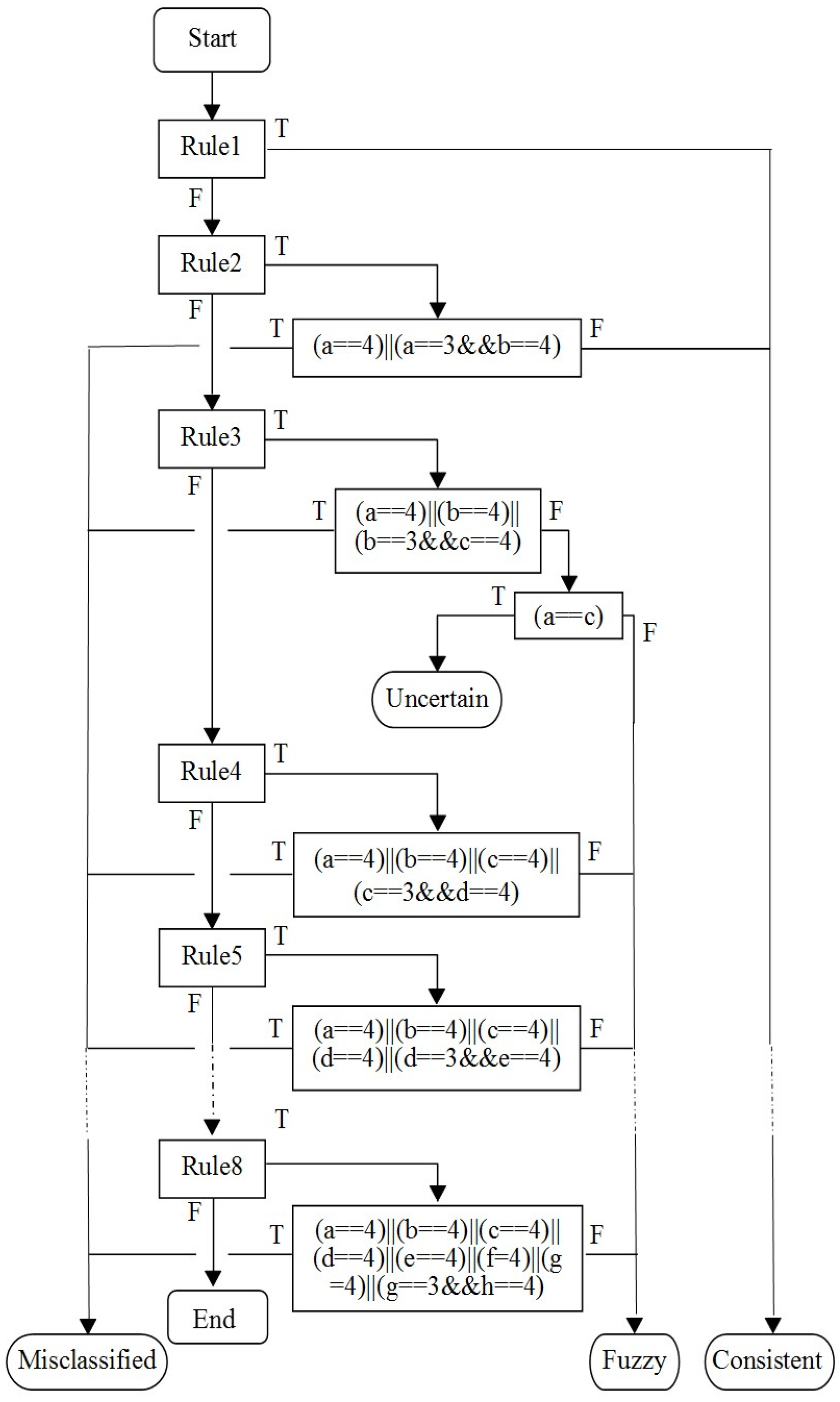
Figure A1, eight rules are employed to assess the rationality of each pixel change. The rules are examined in sequential order.
Figure A1. Rationality evaluation rules.
Forests 07 00218 g005
The eight rules are defined and explained as follows:
Rule 1
If t = 0, then accept “Consistent”.
Rule 2
If t = 1, i.e., T(Ca, Cb), AND if (a==4)||(a==3&&b==4), THEN accept “Misclassified”; otherwise, “Consistent”.
Rule 3
If t = 2, i.e., T(Ca, Cb, Cc), AND if (a==4)||(b==4)||(b==3&&c==4), THEN accept “Misclassified”. Otherwise, check if (a==c). If so, “Uncertain”; otherwise, “Fuzzy”.
Rule 4
If t = 3, i.e., T(Ca, Cb, Cc, Cd), AND if (a==4)||(b==4)||(b==3&&c==4), THEN accept “Misclassified”; otherwise, “Fuzzy”.
Rule 5
If t = 4, i.e., T(Ca, Cb, Cc, Cd, Ce), AND if (a==4)||(b==4)||(c==4)||(d==4)||(d==3&&e==4), THEN accept “Misclassified”; otherwise, “Fuzzy”.
Rule 6
If t = 5, i.e., T(Ca, Cb, Cc, Cd, Ce, Cf), AND if (a==4)||(b==4)||(c==4)||(d==4)||(e==4)||(e==3&&f==4), THEN accept “Misclassified”; otherwise, “Fuzzy”.
Rule 7
If t = 6, i.e., T(Ca, Cb, Cc, Cd, Ce, Cf, Cg), AND if (a==4)||(b==4)||(c==4)||(d==4)||(e==4)||(f=4)||(f==3&&g==4), THEN accept “Misclassified”; otherwise, “Fuzzy”.
Rule 8
If t = 7, i.e., T(Ca, Cb, Cc, Cd, Ce, Cf, Cg, Ch), AND if (a==4)||(b==4)||(c==4)||(d==4)||(e==4)||(f=4)||(g=4)||(g==3&&h==4), THEN accept “Misclassified”; otherwise, “Fuzzy”.
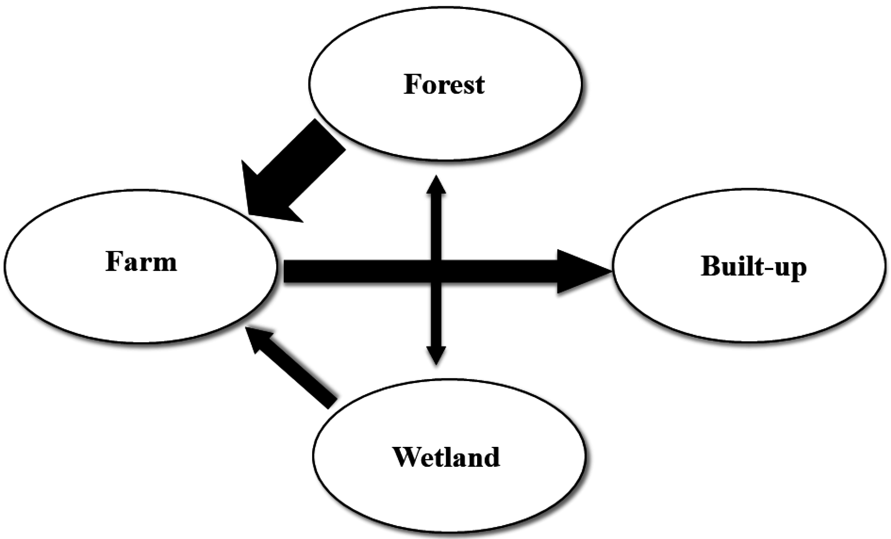
There are two important assumptions behind these eight rules. First, the change to built-up from other land-use classes is irreversible, so that any pixel that is classified as built-up in a previous point of time and later placed into any other land use class would be regarded as a misclassification. Second, it is also uncommon to build on wetland; therefore, conversions from wetland to built-up are all treated as misclassifications.
Rule 1 is straightforward; if a pixel is classified in the same land-use class for all six periods, then the pixel is regarded as “consistent”. Rule 2 concerns the situation when a once-only change is detected for a pixel. If the land conversion direction is true (T) with the two misclassification statements, then the change is labeled “misclassified”. In other cases, we take it as a possible change and thus regard it as correctly classified (“consistent”). Similar to Rule 2, Rule 3 first defines that if the reverse process (i.e., change from built-up area to another land-use type) or the unlikely process (i.e. change from built-up to other) were detected, the change is taken as misclassified. This rule deals with a one-time error of multi-temporal remote sensing image classification. If a pixel is found to have changed from one class (Ca) to another (Cb) and back to its original status (Ca), it could be taken as a one-time classification error (i.e., Cb is the incorrect class), or it could be that the pixel itself is fuzzy and thus could be classified as Ca or Cb. This one-time inconsistent situation does not affect the final result of cover detection, but it is hard to tell whether it is a classification error or not, so the pixel is regarded as “Uncertain”. Finally, Rule 3 specifies the treatment of a case where the land-use type changed twice to two different classes during the whole study period. In this case, we consider the pixel “Fuzzy” with a composite land use type.
Rules 4, 5, 6, 7, and 8 consider pixels that change frequently between cover types. This is most likely a consequence of mis-registration in geometric image rectification (Townshend et al. 1992, Stow 1999). Obviously, the reverse process and the unlikely process would be both improbable according to Rule 2. For other similar pixels, this can be considered as a “Fuzzy” case with frequent cover classes.
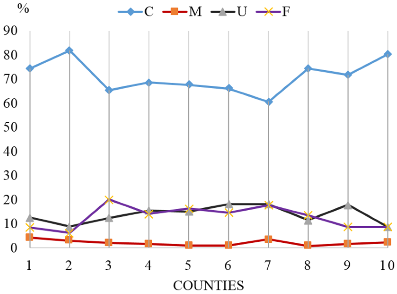
Since, in this study, a county is the basic socioeconomic unit of observation and analysis, the pixel-based results of LULCC detection are represented at the county level in Figure A2 below. Overall, the rationality evaluation accuracy in aggregate are generally acceptable when the “Misclassified” rate is low—less than 5% for all the 10 counties. On average, it is only 1.84% for the whole study area. The pixels classified as “Consistent” account for 70.94% of the total, and “Uncertain” and “Fuzzy” rates are around 14.42% and 12.80%, respectively.
Figure A2. Rule-based rationality evaluation results. C, M, U, F stand for “Consistent”, “Misclassified”, “Uncertain”, and “Fuzzy”, respectively. The ten counties are: Huachuan = 1, Jixian = 2, Shuangyashan City = 3, Huanan = 4, Yilan = 5, Boli = 6, Qitaihe City = 7, Fangzheng = 8, Suibin = 9, and Youyi = 10.
Forests 07 00218 g006
From Figure A2, it is not hard to infer that the “Uncertain” and “Fuzzy” classes are among the most active pixels where land conversion tends to take place. One possible explanation for these high rates is: as most counties in the study region are located alongside the Songhua River, and summer is usually the rainy season, large tracks of farmland on the riverside are flooded, thus the possibility of classifying these pixels as “Uncertain” and “Fuzzy” is larger than other area. Since some of the once-only land use changes determined by Rule 2 are also regarded as “Consistent”, thus, the unchanged land is smaller than the total amount denoted as “consistent”, and the potential LULCC change is possibly larger than that reflected in the proportion of “Uncertain” and “Fuzzy”.
The rule-based rationality evaluation is not only logically sound, but also good at identifying spatially specific areas that are changed and unchanged, especially at recognizing the misclassification, which is helpful for further classification correction. However, there are also deficiencies in this method. The most important one is the difficulty in matching the programming language and semantic meaning used to differentiate different accuracy evaluation scenarios. For example, the “misclassified rate” is defined based on the two most important and logically identifiable cases, but it is not the common misclassification rate as we usually refer to. Also, it is hard to clearly differentiate once-only changes from fuzzy pixels using Rule 3; thus, the “Uncertain” and “Fuzzy” rates are subject to dispute. However, it is not easy to choose the words that exactly match the logic of programming.
Another caveat of interpreting the accuracy evaluation results lies in the image geometric rectification. The multi-temporal image-to-image registration for 1977 and 1984 was controlled in an allowable range with average root mean square error smaller than 0.5; however, potential registration errors still exist in the entire image and could possibly affect the accuracy assessment of those pixels that lie on the frontiers of land conversion (like on the forestland and wetland boundaries).

Appendix B. Accuracy Assessment of Classified LULCC—The Traditional Approach

Due to limitations of the rule-based rational evaluation method, the commonly adopted accuracy assessment scheme is also employed. To validate the accuracy of the classified LULCC results under this method, the simple equation used to estimate sample size is adopted: N = Z α / 2 2 P ( 1 P ) / C I [40]. The overall accuracy P for each class of land use is usually assumed to be 80%. C I is the half width of the confidence interval; a value of 0.05 is often taken. Following the conventional practice, Z α / 2 2 is set at 1.96. The calculated results suggest that sample size for each category should be at least 246. Given the four landscape classes, about 1000 points are thus needed to be drawn from the map of the whole study region.
To this end, the spatially balanced sampling method, which draws sample points proportional to the presence of the area [36], was used to generate 1200 points in the study area. Google Earth was used as the reference data for 2000, 2004, and 2007, respectively (images before 2010 were classified in 2009, whereas images of 2010 and 2013 were classified in 2016). After the layer of randomly sampled points was created, it was converted into a KML file readable by Google Earth and the categories of those points on Google Earth were marked. Next, the extracted Google Earth map information was compared to the classification results [41,42]. Based on the two datasets for the same points, the Kappa indices and conversion matrixes can be derived. During this process, an error in ArcMap 10 occurred, which provided wrong numbers in the attributes table. This led to the density of sampling points being incorrectly estimated, with less than 40 points for the minor LULCC categories (built-up and other). To get a larger sample to alleviate this problem, another 400 randomly generated sample points were added to the two minor categories. In the end, the total sample size reached 1550 points.
For the land-use maps before 2000 (1977, 1984, and 1990), it is not feasible to directly take a reference map from Google Earth, because most images in Google Earth are from after 2000. Because no other kinds of maps were available, it was hard to get a reliable reference for those earlier years. Therefore, we took the following two steps to address the problem. First, note that the four classes of land use are not easily re-convertible. For example, it is highly less likely for forestland to be converted to farmland and then reconverted back to forestland. Thus, the first step was to select those consistent points from a land-use classification map from an earlier period and the Google Earth data from 2004 in the whole sample and take those points as unchanged. The second step was to extract the inconsistent points and compare them with the original images. As the geo-corrected and atmospheric-adjusted images are the best available reference data, the inconsistent points were manually recorded to distinguish points of real change from misclassifications. One thing to be noted here is that due to the lower resolution of MSS data in 1977 and 1984, some confusion occurred in farmland and built-up area, so a compromise is to merge these two classes and assess accuracy of them together as one class.
When the images of 2010 and 2013 were classified in 2016, the first step of selecting consistent points was the same as that of the pre-2000 image accuracy assessment. The second step was altered by taking the newly updated Google Earth images as the reference data. In doing so, time efficiency was gained in step one while the accuracy was improved in the second step.
Based on the above steps, the accuracy assessment results are summarized in Table B1. The overall accuracy rates for the eight points of time are around or above 85%. For 1977 and 1984, as the MSS data have coarser spatial resolution than TM and ETM+ images, we merged farmland and built-up land into one category, called F&B. The overall accuracy based on three classes for 1977 and 1984 is 91.6% and 90.5%, respectively; and the overall Kappa indexes are 86.1% and 84.2%. The classifications of the maps for the other six points of time include four LULCC categories: farmland, forestland, built-up land, and other. The overall accuracy rates for these six periods are around 85%, and the Kappa indexes are about 80%. Given the large sample size, the standard deviations and coefficients of variation for both overall accuracy and Kappa indexes are very small.
Table B1. Overall accuracy assessment of the LULCC classification results.
YearOA 1 (%)Std 2 (10−2)CV 3 (%)Kappa (%)Std (10−2)CV (%)
1977 491.610.700.7686.141.160.74
1984 590.520.740.8284.171.240.68
199387.810.830.9582.211.210.68
200084.240.931.1077.151.350.57
200486.240.881.0280.091.280.63
200789.080.790.8984.441.130.75
201088.630.810.9083.661.161.40
201386.430.871.0080.381.261.60
1 OA stands for overall accuracy; 2 Std for standard deviation; 3 and CV for coefficient of variation showing the extent of variability in relation to the overall accuracy; 4,5 Classes of farmland and built-up in the periods of 1977 and 1984 were merged together due to the coarse resolution of MSS data.
The class-specific land use accuracy results are summarized in Table B2 and Table B3, respectively. In both tables, the left block is the common confusion matrix [43]; the middle block contains the calculated indices of user’s accuracy (UA); and the right block contains the indices of producer’s accuracy (PA). To be thorough, the tables also include the Kappa index reflecting the difference between the classification agreement and the agreement expected by chance [44]. Some authors argue that this index tends to underestimate the accuracy [45]. The calculated values are generally lower than those from the UA and PA statistics.
Table B2. LULCC category-based accuracy assessment for 1977 and 1984.
F&BFtOtherUAKappaStdPRKappaStd
F&B70516180.950.910.020.890.780.02
1977Ft6351340.880.820.020.970.950.01
Other2812010.870.850.030.900.880.02
F&B74112290.950.890.020.880.760.02
1984Ft6145970.870.810.020.970.960.01
Other3802030.840.810.030.850.820.03
F&B stands for farmland and built-up, Ft for forest, and other includes wetland, grassland, and unused land. UA and PA stand for user’s and producer’s accuracy, respectively. Std stands for standard deviation. The number of observations was 1549 in 1977 and 1550 in 1984.
Table B3. LULCC category-based accuracy assessment for later years.
FmFtOtherBltupUAKappaStdPRKappaStd
1993Fm5851565190.860.750.020.890.80.02
Ft33443530.920.880.020.960.950.01
Other28117010.850.820.030.690.650.03
Bltup12161630.90.880.030.880.860.03
2000Fm5593836120.870.760.020.810.670.02
Ft64393250.850.790.020.890.840.02
Other56918630.730.690.030.810.780.03
Bltup13151660.90.880.030.890.880.03
2004Fm564303070.890.810.020.820.690.02
Ft63406270.850.790.020.920.890.02
Other50419520.780.740.030.850.820.03
Bltup15121700.90.890.020.910.90.02
2007Fm56113630.960.930.010.810.70.02
Ft43422300.90.860.020.960.940.01
Other71421650.730.680.030.950.940.02
Bltup17221800.90.880.020.960.950.02
2010Fm5691233170.900.830.020.870.780.02
Ft39429910.900.850.020.940.910.02
Other371419820.790.750.030.830.790.03
Bltup11101760.940.930.020.900.880.02
2013Fm5661733150.900.810.020.820.690.02
Ft56415520.870.820.020.940.910.02
Other54718820.750.710.030.830.790.03
Bltup16211690.900.890.020.900.890.02
Fm stands for farmland, Ft for forestland, Bltup for built-up, and other for wetland, grassland and unused land; UA and PA stand for user’s and producer’s accuracy; and Std stands for standard deviation.
It can be seen from Table B3 that the classification of farmland and forestland—the focal classes of land use—is reasonably good, with most having an accuracy rate higher than 85%. The accuracy for built-up land is also reasonable after the 1990s, with all the accuracy rates above 90%. The minor category of other land, mainly wetland, has a relatively lower accuracy rate. One explanation is related to the seasonal change: because the dates of the images acquired deviate from those of the reference Google maps, some farmland and wetland along the Songhua River could have different boundaries. Meanwhile, in a 30-by-30-m pixel, some sub-pixel areas may include more than one land use classes. Lastly, small positional deviations between Landsat images and images in Google Earth could also be a potential source for lower accuracy [46,47].

References

  1. Liu, J.; Diamond, J. China’s environment in a globalizing world. Nature 2005, 435, 1179–1186. [Google Scholar] [CrossRef] [PubMed]
  2. Xu, J.; Yin, R.; Li, Z.; Liu, C. China’s ecological rehabilitation: The unprecedented efforts and dramatic impacts of reforestation and slope protection in western China. Ecol. Econ. 2005, 57, 595–607. [Google Scholar] [CrossRef]
  3. Yin, R.; Yin, G. China’s ecological restoration programs: Initiation, implementation, and challenges. In An Integrated Assessment of China’s Ecological Restoration Programs; Springer: Berlin, Germany, 2009; pp. 1–19. [Google Scholar]
  4. Yamane, M. China’s recent forest-related policies: Overview and background. Policy Trend Rep. 2001, 1, 1–12. [Google Scholar]
  5. Yin, R.; Yin, G. China’s primary programs of terrestrial ecosystem restoration: Initiation, implementation, and challenges. Environ. Manag. 2010, 45, 429–441. [Google Scholar] [CrossRef] [PubMed]
  6. Trac, C.J.; Schmidt, A.H.; Harrell, S.; Hinckley, T.M. Environmental reviews and case studies: Is the returning farmland to forest program a success? Three case studies from sichuan. Environ. Pract. 2013, 15, 350–366. [Google Scholar] [CrossRef] [PubMed]
  7. Zhang, P.; Shao, G.; Zhao, G.; Le Master, D.C.; Parker, G.R.; Dunning, J.B., Jr.; Li, Q. China’s forest policy for the 21st century. Science 2000, 288, 2135–2136. [Google Scholar] [CrossRef] [PubMed]
  8. State Forestry Administration (SFA). Statistics on the National Forest Resources (the 5th National Forest Inventory 1994–1998); State Forestry Administration: Beijing, China, 2000. (In Chinese)
  9. Delang, C.O.; Yuan, Z. China’s reforestation and rural development programs. In China’s Grain for Green Program; Springer: Berlin, Germany, 2015; pp. 19–35. [Google Scholar]
  10. Zhang, K.; Hori, Y.; Zhou, S.; MiChinaka, T.; Hirano, Y.; Tachibana, S. Impact of natural forest protection program policies on forests in northeastern China. For. Stud. China 2011, 13, 231–238. [Google Scholar] [CrossRef]
  11. Edström, F.; Nilsson, H.; Stage, J. The natural forest protection program in China: A contingent valuation study in heilongjiang province. J. Environ. Sci. Eng. 2012, 1, 426–432. [Google Scholar]
  12. NFPP Management Center. Authoritative Interpretations for the Second Phase Policies of Natural Forest Protection Project. (In Chinese). Available online: http://www.forestry.gov.cn/ZhuantiAction.do?dispatch=content&id=484664&name=trlbhgc (accessed on 11 June 2015).
  13. Wang, Z.; Wu, J.; Madden, M.; Mao, D. China’s wetlands: Conservation plans and policy impacts. Ambio 2012, 41, 782–786. [Google Scholar] [CrossRef] [PubMed]
  14. Huang, W.; Deng, X.; Lin, Y.; Jiang, Q. An econometric analysis of causes of forestry area changes in northeast China. Procedia Environ. Sci. 2010, 2, 557–565. [Google Scholar] [CrossRef]
  15. Mullan, K.; Kontoleon, A.; Swanson, T.; Zhang, S. An evaluation of the impact of the natural forest protection programme on rural household livelihoods. In An Integrated Assessment of China’s Ecological Restoration Programs; Springer: Berlin, Germany, 2009; pp. 175–199. [Google Scholar]
  16. Jiang, X.; Gong, P.; Bostedt, G.; Xu, J. Impacts of policy measures on the development of state-owned forests in northeast China: Theoretical results and empirical evidence. Environ. Dev. Econ. 2014, 19, 74–91. [Google Scholar] [CrossRef]
  17. Tang, J.; Wang, L.; Zhang, S. Investigating landscape pattern and its dynamics in daqing, China. Int. J. Remote Sens. 2005, 26, 2259–2280. [Google Scholar] [CrossRef]
  18. Wang, Z.; Zhang, B.; Zhang, S.; Li, X.; Liu, D.; Song, K.; Li, J.; Li, F.; Duan, H. Changes of land use and of ecosystem service values in sanjiang plain, northeast China. Environ. Monit. Assess. 2006, 112, 69–91. [Google Scholar] [CrossRef] [PubMed]
  19. Wang, Z.; Liu, Z.; Song, K.; Zhang, B.; Zhang, S.; Liu, D.; Ren, C.; Yang, F. Land use changes in northeast China driven by human activities and climatic variation. Chin. Geogr. Sci. 2009, 19, 225–230. [Google Scholar] [CrossRef]
  20. Okamoto, K.; Kawashima, H. Estimating total area of paddy fields in heilongjiang, China, around 2000 using landsat thematic mapper/enhanced thematic mapper plus data. Remote Sens. Lett. 2016, 7, 533–540. [Google Scholar] [CrossRef]
  21. Dan, W.; Wei, H.; Shuwen, Z.; Kun, B.; Bao, X.; Yi, W.; Yue, L. Processes and prediction of land use/land cover changes (LUCC) driven by farm construction: The case of Naoli River basin in Sanjiang Plain. Environ. Earth Sci. 2015, 73, 4841–4851. [Google Scholar] [CrossRef]
  22. Song, k.; Wang, Z.; Liu, Q.; Lu, D.; Yang, G.; Zeng, L.; Liu, D.; Zhang, B.; Du, J. Land use/land cover (LULC) characterizaitoin with modis time series data in the amu river basin. In Proceedings of the 2009 International Geoscience and Remote Sensing Symposium, Cape Town, South Africa, 12–17 July 2009; IV, pp. 310–313.
  23. Wang, Z.; Song, K.; Ma, W.; Ren, C.; Zhang, B.; Liu, D.; Chen, J.M.; Song, C. Loss and fragmentation of marshes in the sanjiang plain, northeast China, 1954–2005. Wetlands 2011, 31, 945–954. [Google Scholar] [CrossRef]
  24. Zhou, Z.; Liu, T. The current status, threats and protection way of sanjiang plain wetland, northeast China. J. For. Res. 2005, 16, 148–152. [Google Scholar]
  25. Zhou, D.; Gong, H.; Wang, Y.; Khan, S.; Zhao, K. Driving forces for the marsh wetland degradation in the honghe national nature reserve in sanjiang plain, northeast China. Environ. Model. Assess. 2009, 14, 101–111. [Google Scholar] [CrossRef]
  26. Yin, R. Forestry and the environment in China: The current situation and strategic choices. World Dev. 1998, 26, 2153–2167. [Google Scholar] [CrossRef]
  27. Chinese Academy of Sciences. China Remote Sensing Satellite Ground Station; Chinese Academy of Sciences: Beijing, China, 2008. [Google Scholar]
  28. U.S. Department of the Interior. U.S. Geological Survey, 2009. Availabe online: http://glovis.usgs.gov/index.shtm (accessed on 24 February 2016).
  29. Gong, P.; Wang, J.; Yu, L.; Zhao, Y.; Zhao, Y.; Liang, L.; Niu, Z.; Huang, X.; Fu, H.; Liu, S. Finer resolution observation and monitoring of global land cover: First mapping results with landsat tm and ETM+ data. Int. J. Remote Sens. 2013, 34, 2607–2654. [Google Scholar] [CrossRef]
  30. Chavez, P.S. Image-based atmospheric corrections-revisited and improved. Photogramm. Eng. Remote Sens. 1996, 62, 1025–1035. [Google Scholar]
  31. Song, C.; Woodcock, C.E.; Seto, K.C.; Lenney, M.P.; Macomber, S.A. Classification and change detection using landsat tm data: When and how to correct atmospheric effects? Remote Sens. Environ. 2001, 75, 230–244. [Google Scholar] [CrossRef]
  32. Deng, J.; Wang, K.; Deng, Y.; Qi, G. Pca-based land-use change detection and analysis using multitemporal and multisensor satellite data. Int. J. Remote Sens. 2008, 29, 4823–4838. [Google Scholar] [CrossRef]
  33. Anderson, J.R.; Hardy, E.E.; Roach, J.T.; Witmer, R.E. A land use and land cover classification system for use with remote sensor data. In Geological Survey Professional Paper; USGS: Reston, VA, USA, 1976; Volume 964. [Google Scholar]
  34. Pontius, R.G.; Shusas, E.; McEachern, M. Detecting important categorical land changes while accounting for persistence. Agric. Ecosyst. Environ. 2004, 101, 251–268. [Google Scholar] [CrossRef]
  35. Liu, H.; Zhou, Q. Accuracy analysis of remote sensing change detection by rule-based rationality evaluation with post-classification comparison. Int. J. Remote Sens. 2004, 25, 1037–1050. [Google Scholar] [CrossRef]
  36. Stevens, D.L., Jr.; Olsen, A.R. Spatially balanced sampling of natural resources. J. Am. Stat. Assoc. 2004, 99, 262–278. [Google Scholar] [CrossRef]
  37. World Resources Institute. Global Forest Watch, 2014. Available online: http//www.Globalforestwatch.Org (accessed on 5 May 2016).
  38. Chavez, P.; Sides, S.C.; Anderson, J.A. Comparison of three different methods to merge multiresolution and multispectral data-landsat tm and spot panchromatic. Photogramm. Eng. Remote Sens. 1991, 57, 295–303. [Google Scholar]
  39. Foody, G.M. Assessing the accuracy of land cover change with imperfect ground reference data. Remote Sens. Environ. 2010, 114, 2271–2285. [Google Scholar] [CrossRef]
  40. Foody, G.M. Sample size determination for image classification accuracy assessment and comparison. Int. J. Remote Sens. 2009, 30, 5273–5291. [Google Scholar] [CrossRef]
  41. Boulos, M.N. Web GIS in practice III: Creating a simple interactive map of England’s Strategic Health Authorities using Google Maps API, Google Earth KML, and MSN Virtual Earth Map Control. Int. J. Health Geogr. 2005, 4, 22. [Google Scholar] [CrossRef] [PubMed]
  42. Du, Y.; Yu, C.; Jie, L. A study of gis development based on kml and google earth. In Proceedings of the Fifth International Joint Conference on INC, IMS and IDC (NCM’09), Seoul, Korea, 25–27 August 2009; pp. 1581–1585.
  43. Foody, G.M. Status of land cover classification accuracy assessment. Remote Sens. Environ. 2002, 80, 185–201. [Google Scholar] [CrossRef]
  44. Stehman, S.V. Selecting and interpreting measures of thematic classification accuracy. Remote Sens. Environ. 1997, 62, 77–89. [Google Scholar] [CrossRef]
  45. Rosenfield, G.H.; Fitzpatrick-Lins, K. A coefficient of agreement as a measure of thematic classification accuracy. Photogramm. Eng. Remote Sens. 1986, 52, 223–227. [Google Scholar]
  46. Dai, X.; Khorram, S. The effects of image misregistration on the accuracy of remotely sensed change detection. IEEE Trans. Geosci. Remote Sens. 1998, 36, 1566–1577. [Google Scholar]
  47. Potere, D. Horizontal positional accuracy of google earth’s high-resolution imagery archive. Sensors 2008, 8, 7973–7981. [Google Scholar] [CrossRef]
Figure 1. Study site in Heilongjiang, northeast China.
Forests 07 00218 g001
Figure 2. Classified land use and land cover change maps of the study region in 1977, 2000, and 2013.
Forests 07 00218 g002
Figure 3. The trajectories of classified farmland, forestland, built-up land, and other land between 1977 and 2013.
Forests 07 00218 g003
Figure 4. Dominant relationships between the land-use classes.
Forests 07 00218 g004
Table 1. Land-use changes over time with estimated gains for each category.
2013Losses
1977 Total 1977FarmForestOtherBuilt-up
FarmO 149.2742.982.100.593.616.29
E 247.9742.982.330.432.234.99
O – E 31.300.00−0.240.151.381.30
(O – E)/E 42.710.00−10.2235.7362.1826.04
ForestO42.3510.7230.770.220.6511.58
E45.4012.3530.770.371.9114.63
O – E−3.05−1.630.00−0.15−1.27−3.05
(O – E)/E−6.72−13.220.00−40.36−66.20−20.83
OtherO7.033.560.612.660.204.37
E5.362.050.332.660.322.70
O – E1.671.510.280.00−0.121.67
(O – E)/E31.0773.4883.350.00−37.0061.71
Built-upO1.350.520.030.010.800.55
E1.270.390.060.010.800.47
O – E0.080.13−0.040.000.000.08
(O – E)/E6.5232.03−60.90−37.760.0017.61
Total 2013O10057.7733.503.485.2622.80
E10057.7733.503.485.2622.80
O – E0.000.000.000.000.000.00
(O – E)/E0.000.000.000.000.000.00
GainsO22.8014.792.730.824.46
E22.8014.792.730.824.46
O – E0.000.000.000.000.00
(O – E)/E0.000.000.000.000.00
1 The bold figures are the observed percentages (O); 2 the regular figures are the expected percentages (E) under the assumption that the loss to each category is random. The expected losses were calculated according to Equation (2); 3 the figures in both bold and italics are the difference (O – E) between the observed and the expected values; 4 and the figures in italics only are the result of the differences divided by the expected values (O – E)/E, multiplied by 100%. The cell blocks in light gray are the diagonal blocks in the conversion matrix and those in dark gray are particularly in the text.
Table 2. Land-use changes over time with estimated losses for each category.
2013Losses
1977 Total 1977FarmForestOtherBuilt-up
FarmO 149.2742.982.100.593.616.29
E 249.2742.984.990.520.786.29
O – E 30.000.00−2.890.072.830.00
(O – E)/E 40.000.00−58.0113.15360.980.00
ForestO42.3510.7230.770.220.6511.58
E42.3510.0630.770.610.9211.58
O – E0.000.650.00−0.38−0.270.00
(O – E)/E0.006.490.00−63.45−29.370.00
OtherO7.033.560.612.660.204.37
E7.032.611.522.660.244.37
O – E0.000.94−0.900.00−0.040.00
(O – E)/E0.0036.07−59.710.00−15.860.00
Built-upO1.350.520.030.010.800.55
E1.350.340.200.020.800.55
O – E0.000.18−0.17−0.010.000.00
(O – E)/E0.0054.39−87.19−63.650.000.00
Total 2013O10057.7733.503.485.26
E10055.9937.473.812.74
O – E0.001.78−3.97−0.332.52
(O – E)/E0.003.18−10.60−8.6592.08
GainsO22.8014.792.730.824.46
E22.8013.016.701.141.94
O – E0.001.78−3.97−0.332.52
(O – E)/E0.0013.67−59.25−28.77130.13
1 The bold figures are the observed percentages (O); 2 the regular figures are the expected percentages (E) under the assumption that the loss to each category is random. The expected losses were calculated according to Equation (2); 3 the figures in both bold and italics are the difference (O – E) between the observed and the expected values; 4 and the figures in italics only are the result of the differences divided by the expected values (O – E)/E, multiplied by 100%. The cell blocks in light gray are the diagonal blocks in the conversion matrix and those in dark gray are particularly noted in the text.
Table 3. Percentages of gains, losses, net changes, and swaps of different land uses.
19772013GainsLossesTotal ChangeNetSwap
Farm49.2757.7714.796.2921.088.5012.58
Forest42.3533.502.7311.5814.32−8.855.46
Other7.033.480.824.375.18−3.551.63
Built-up1.355.264.460.555.013.901.11
Total100.00100.0022.8022.8045.590.0020.78
Table 4. Percentages of gains, losses, net changes, and swaps of different land uses before and after the Natural Forest Protection Program (NFPP) was initiated.
PeriodClassesTime 1Time 2GainsLossesTotal ChangeNetSwap
1993–2000Farm56.1157.857.615.8713.481.7411.74
Forest35.5833.723.965.829.78−1.867.93
Built-up3.343.880.950.421.370.540.83
Other4.964.541.431.853.28−0.422.86
Total10010013.9513.9527.904.5523.36
2000–2007Farm57.8559.236.395.0111.401.3810.02
Forest33.7232.764.245.219.45−0.978.48
Built-up3.884.861.070.101.170.970.20
Other4.543.160.331.722.05−1.390.66
Total10010012.0312.0324.074.7119.36
Difference 1Farm−1.74−1.381.220.862.080.361.72
Forest1.860.96−0.280.610.330.89−0.55
Built-up−0.54−0.98−0.120.320.20−0.430.63
Other0.421.381.100.131.23−0.972.20
Total0.000.001.921.923.83−0.164.00
1 Differences resulted from the values from 1993 to 2000 minus the values from 2000 to 2007.

