
Fire Regime along Latitudinal Gradients of Continuous to Discontinuous Coniferous Boreal Forests in Eastern Canada


Abstract
:1. Introduction
2. Materials and Methods
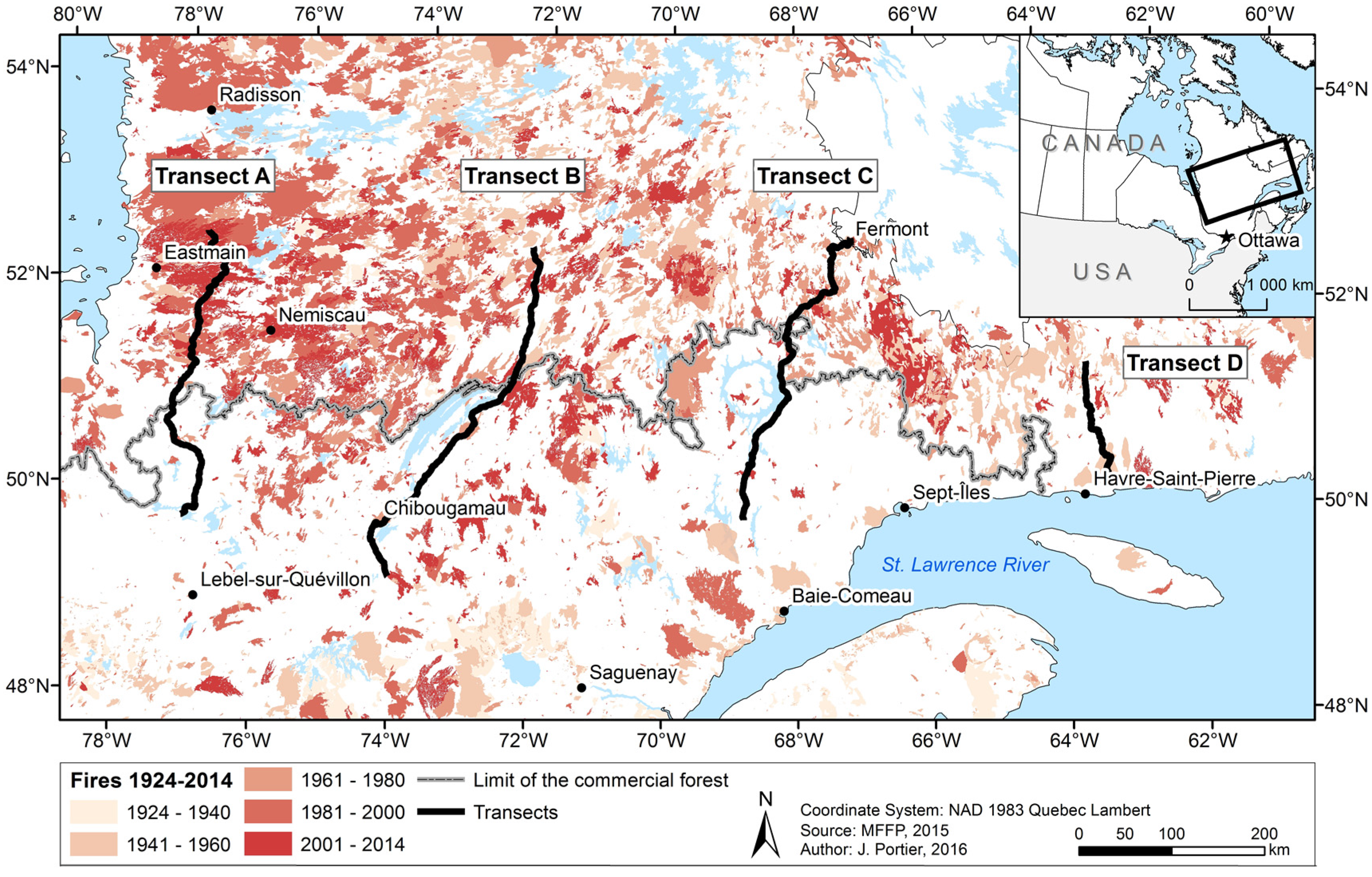
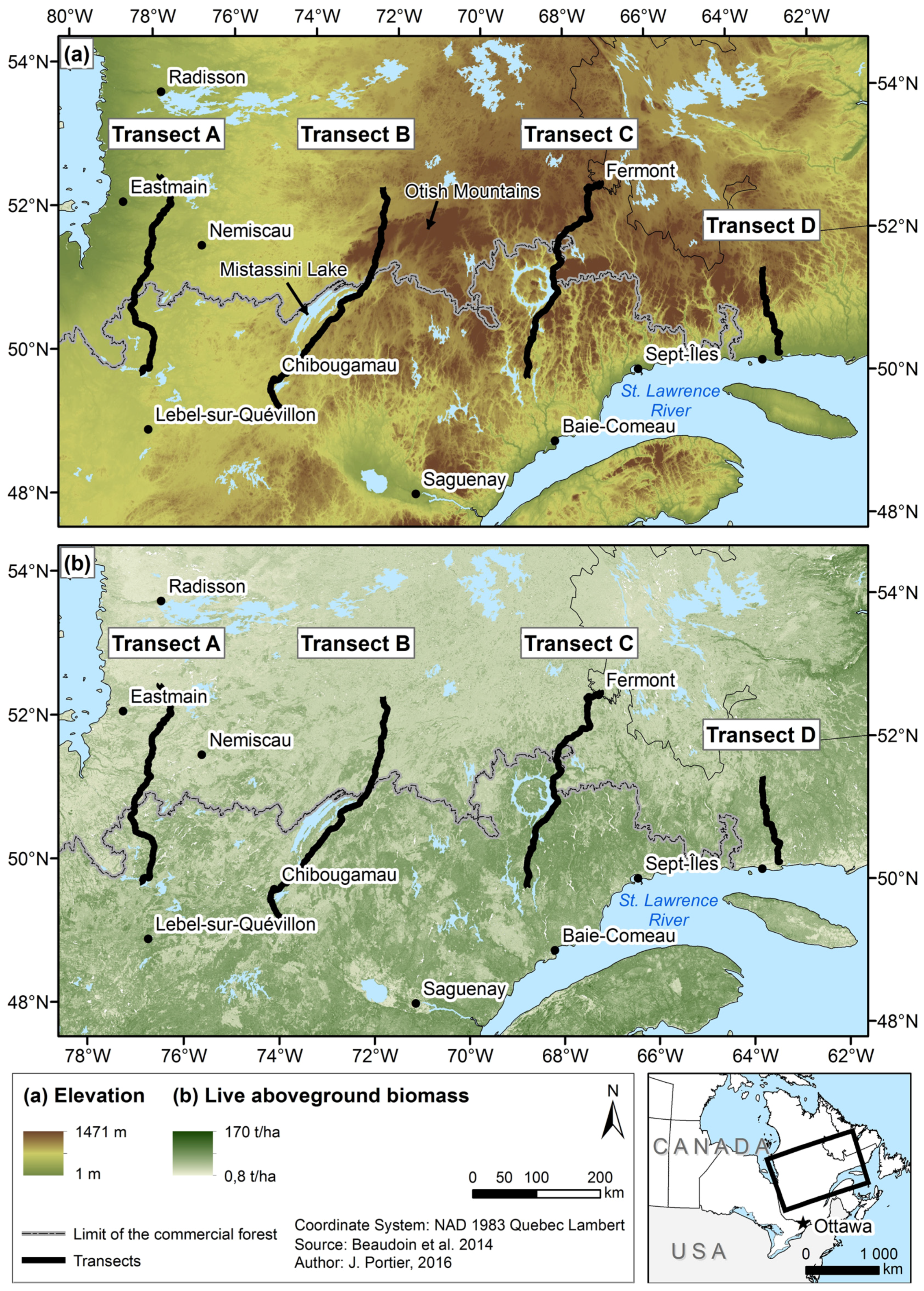
2.1. Study Area
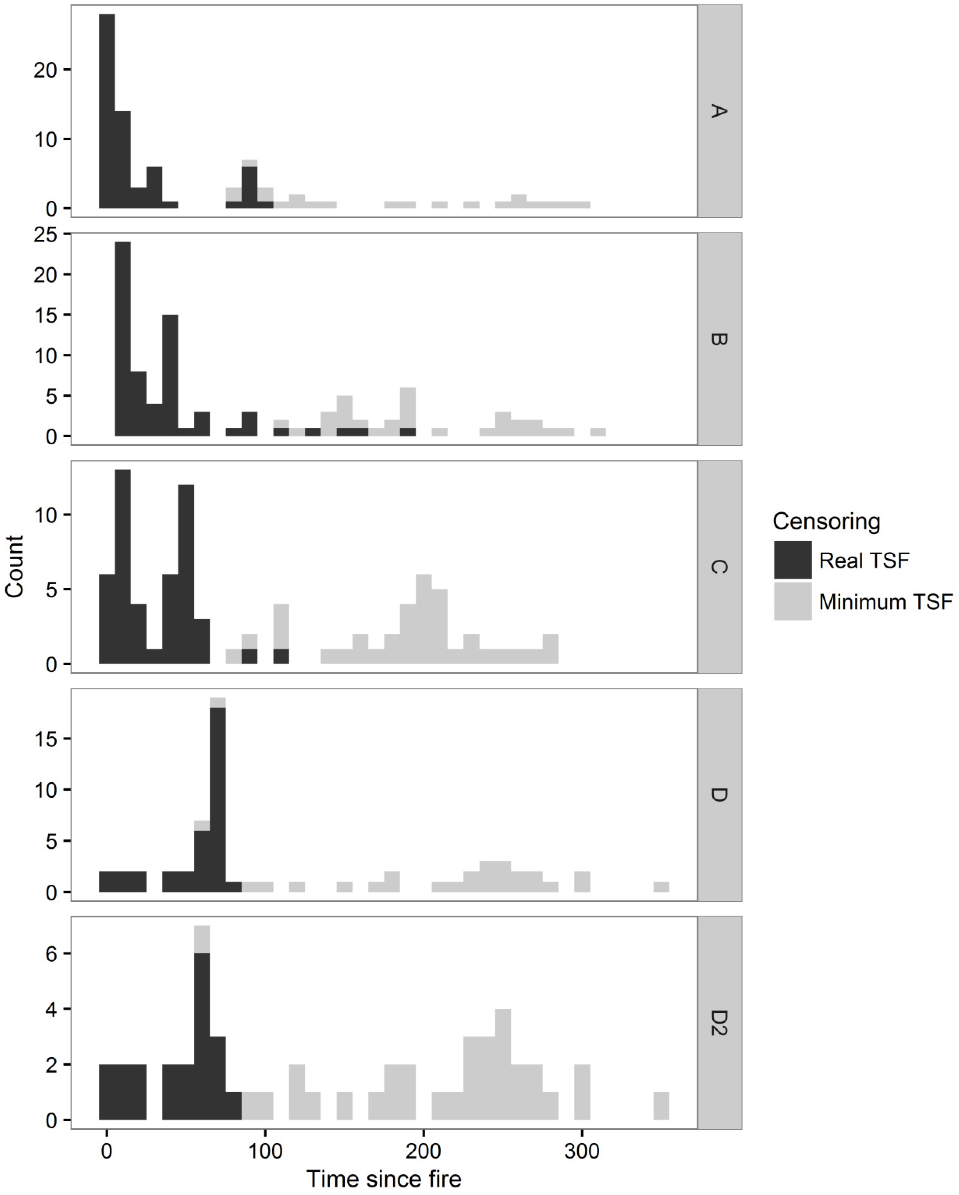
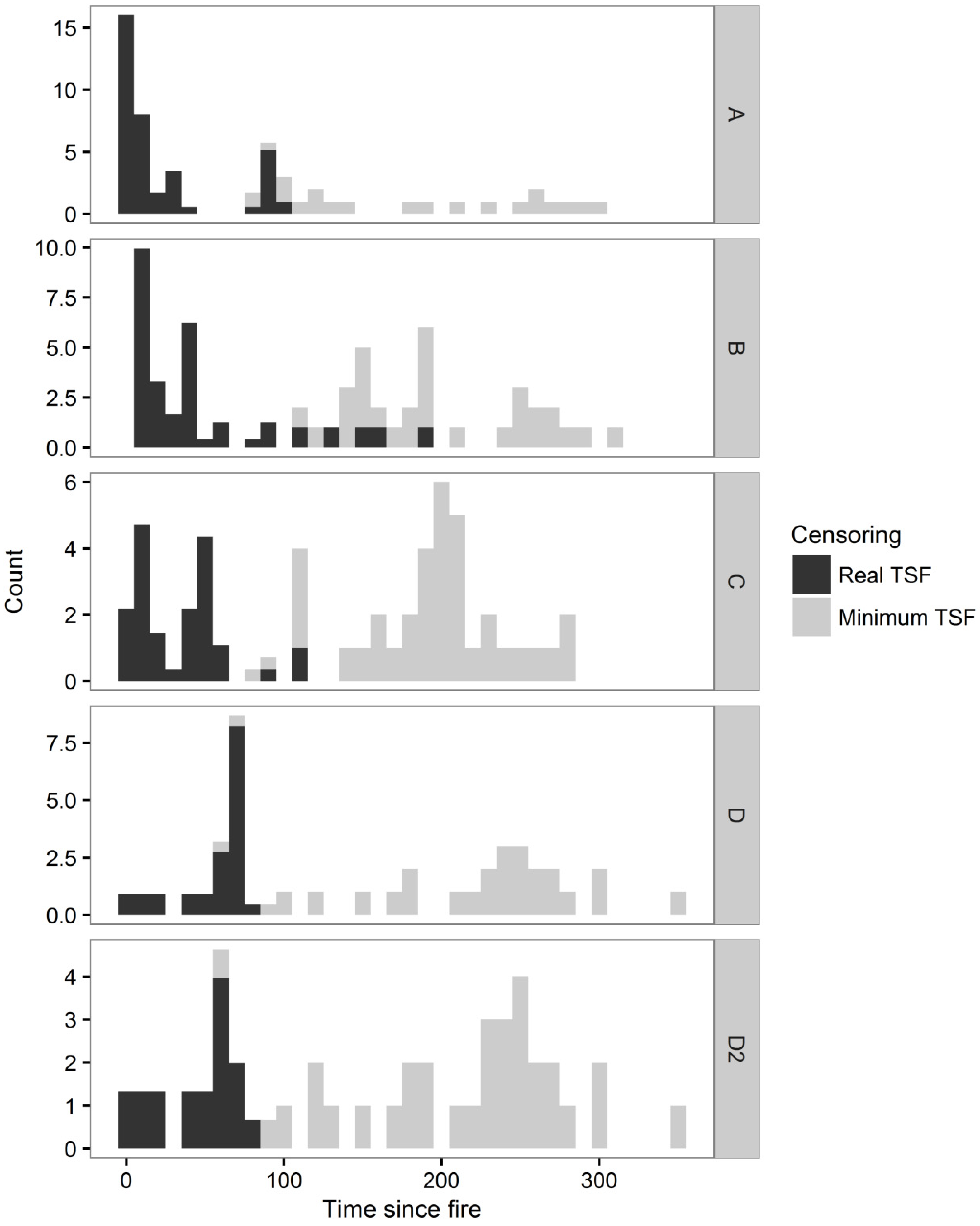
2.2. Time-Since-Fire Data
2.2.1. Fire Archive Data (1924–2014)
2.2.2. Field Sampling Design
2.2.3. Relative Importance of Recent Fires
2.3. Climate Data
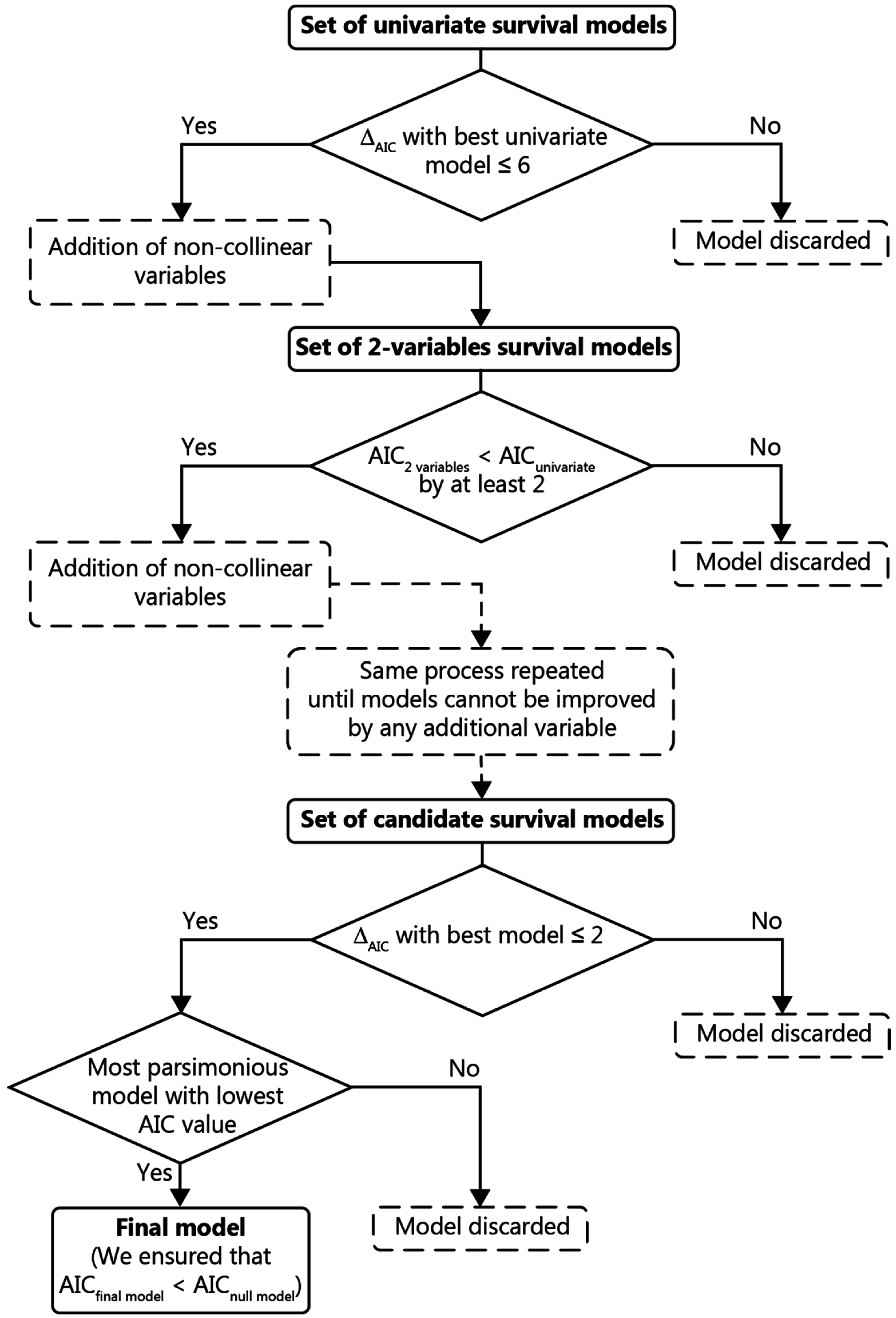
2.4. Statistical Analyses
2.4.1. Climate Influence on Fire Risk
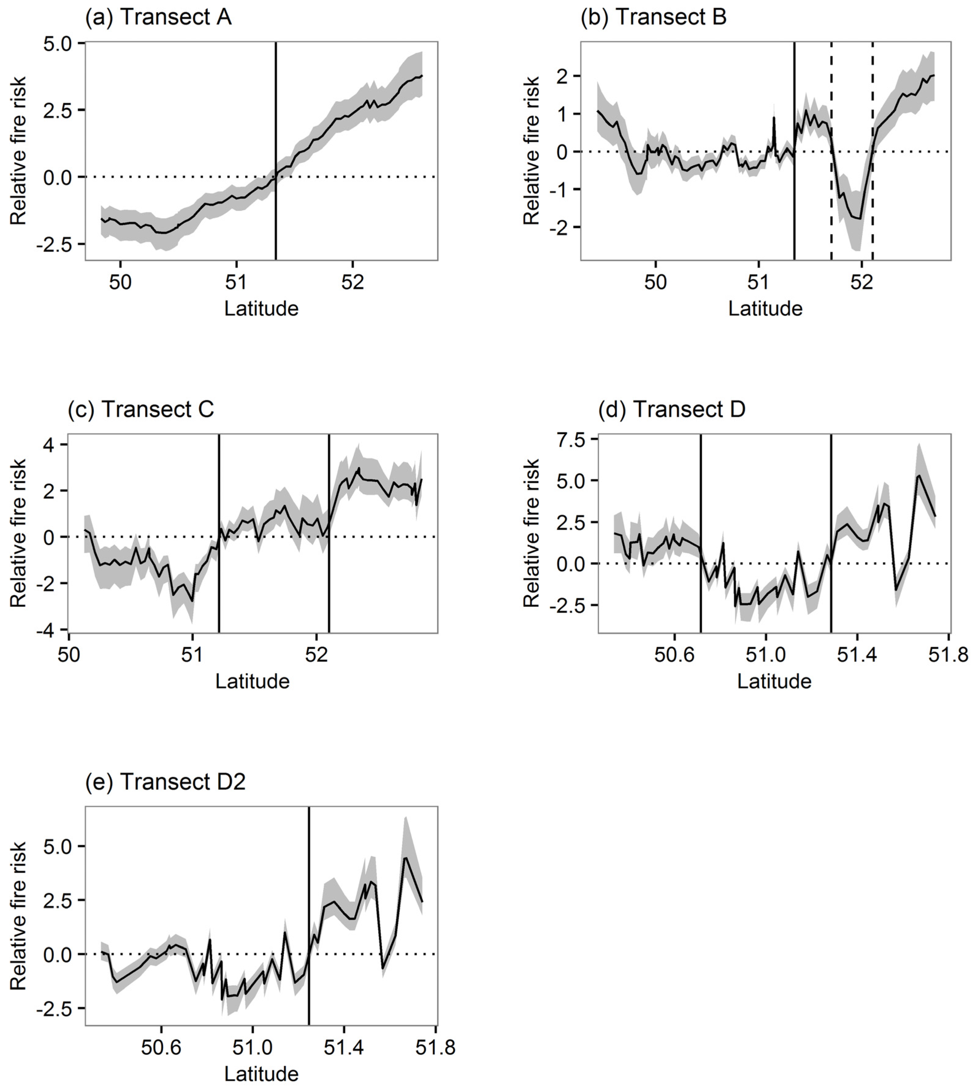
2.4.2. Relative Fire Risk and Latitudinal Risk Zonation
2.4.3. Fire Cycle
3. Results
3.1. Climate Influence on Fire Risk
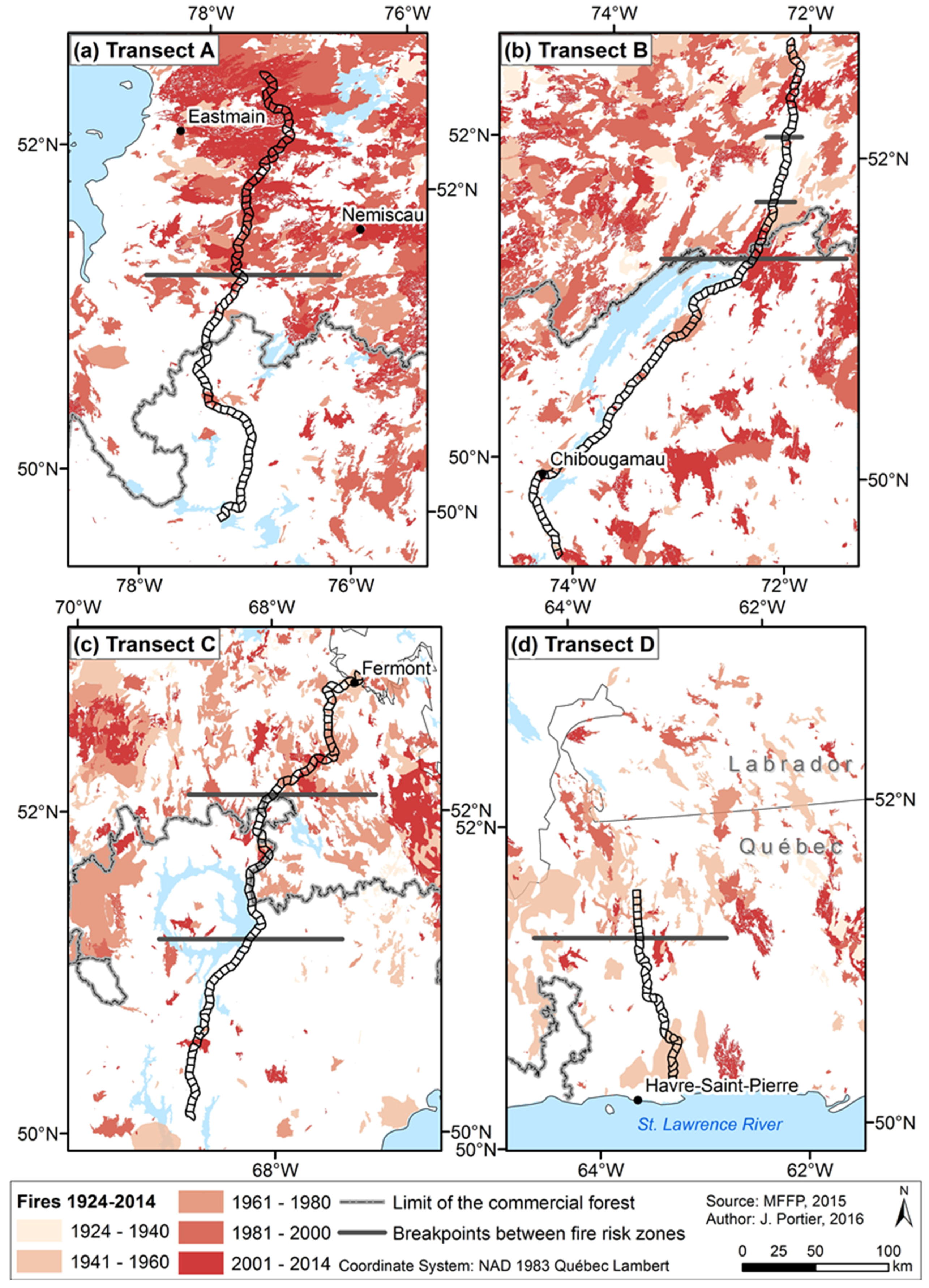
3.2. Relative Fire Risk and Latitudinal Risk Zonation
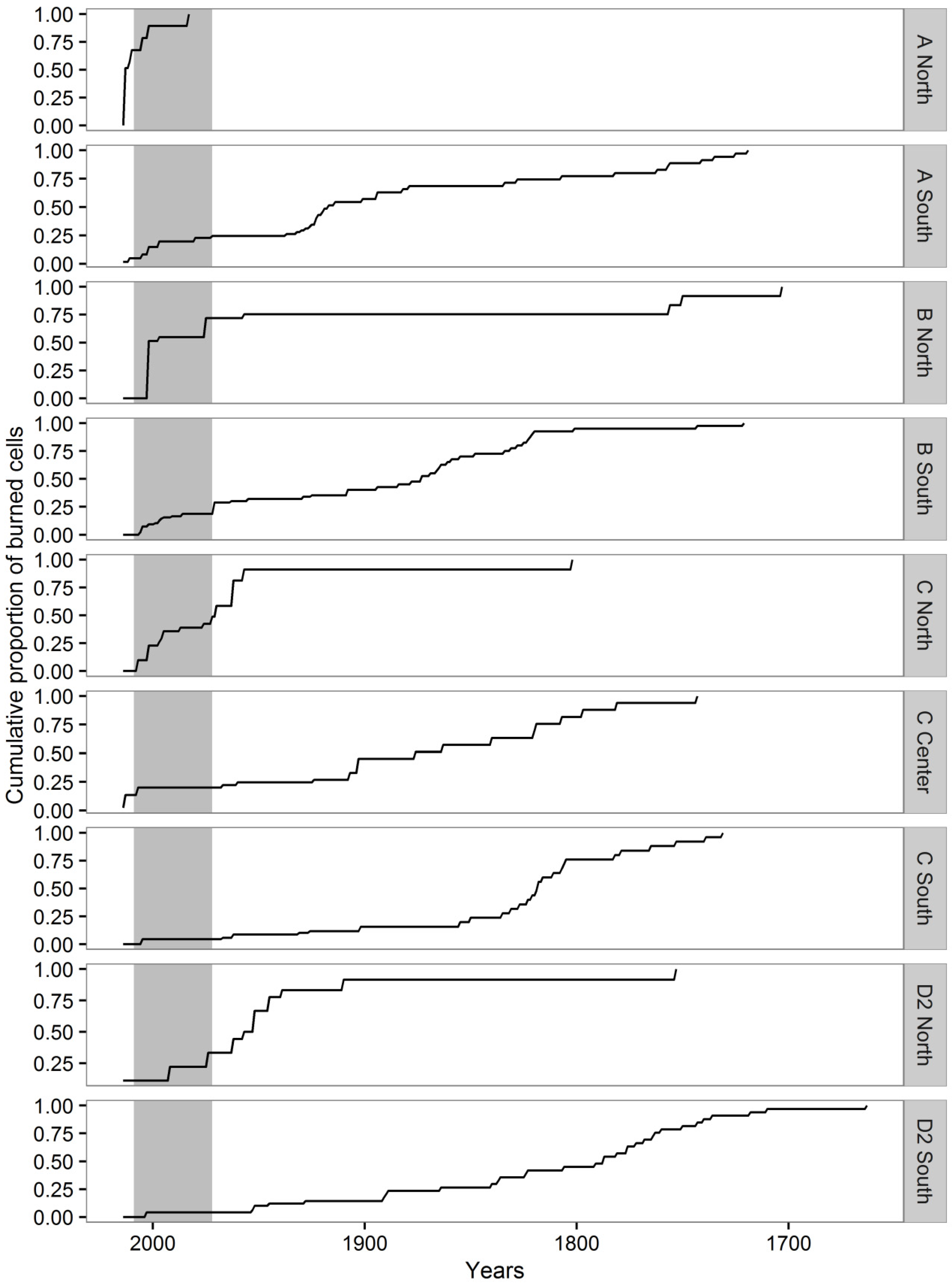
3.3. Fire Cycles
4. Discussion
4.1. Climate Influence on Fire Risk
4.2. Fire Cycle
4.3. Fire Risk Zonation and Temporal Variability
5. Conclusions
Acknowledgments
Author Contributions
Conflicts of Interest
Abbreviations
| AIC | Akaike Information Criterion |
| BUI | Buildup Index |
| CI | Confidence Interval |
| DC | Drought Code |
| DMC | Duff Moisture Code |
| FC | Fire Cycle |
| FFMC | Fine Fuel Moisture Code |
| FWI | Fire Weather Index |
| ISI | Initial Spread Index |
| MFFP | Ministère des Forêts, de la Faune et des Parcs (Québec) |
| TSF | Time Since Fire |
Appendix A


| Transect | Zone | Mean Relative Risk | CI95 |
|---|---|---|---|
| A | North | 15.61 | (7.96; 34.91) |
| South | 0.30 (−3.33) | (0.18; 0.47) | |
| B | North | 3.70 | (2.16; 6.76) |
| Plateau | 0.33 (−3.03) | (0.18; 0.59) | |
| South | 1.05 | (0.75; 1.56) | |
| C | North | 10.48 | (5.29; 24.09) |
| Center | 1.92 | (1.00; 4.09) | |
| South | 0.38 (−2.63) | (0.19; 0.70) | |
| D | North | 48.14 | (14.66; 306.15) |
| South | 0.57 (−1.75) | (0.29; 1.06) | |
| 1940s fire | 3.75 | (1.59; 11.64) | |
| D2 | North | 21.30 | (8.40; 98.19) |
| South | 0.69 (−1.45) | (0.43; 1.16) |
References
- Johnson, E.A. Fire and Vegetation Dynamics: Studies from the North American Boreal Forest; Cambridge: Cambridge, UK, 1992. [Google Scholar]
- Payette, S. Fire as a controlling process in the North American boreal forest. In A System Analysis of the Global Boreal Forest; Shugart, H.H., Leemans, R., Bonan, G.B., Eds.; Cambridge University Press: Cambridge, UK, 1992; pp. 144–169. [Google Scholar]
- Gauthier, S.; Leduc, A.; Bergeron, Y. Forest dynamics modelling under natural fire cycles: A tool to define natural mosaic diversity for forest management. Environ. Monit. Assess. 1996, 39, 417–434. [Google Scholar] [CrossRef] [PubMed]
- Johnson, E.A.; Miyanishi, K.; Weir, J.M.H. Wildfires in the western Canadian boreal forest: Landscape patterns and ecosystem management. J. Veg. Sci. 1998, 9, 603–610. [Google Scholar] [CrossRef]
- Johnson, E.A.; Gutsell, S.L. Fire frequency models, methods and interpretations. Adv. Ecol. Res. 1994, 25, 239–287. [Google Scholar]
- Li, C. Estimation of fire frequency and fire cycle: A computational perspective. Ecol. Modell. 2002, 154, 103–120. [Google Scholar] [CrossRef]
- Van Wagner, C.E. Age-Class distribution and the forest fire cycle. Can. J. For. Res. 1978, 8, 220–227. [Google Scholar] [CrossRef]
- Cyr, D.; Gauthier, S.; Bergeron, Y.; Carcaillet, C. Forest management is driving the eastern North American boreal forest outside its natural range of variability. Front. Ecol. Environ. 2009, 7, 519–524. [Google Scholar] [CrossRef]
- Bouchard, M.; Pothier, D.; Gauthier, S. Fire return intervals and tree species succession in the North Shore region of eastern Quebec. Can. J. For. Res. 2008, 38, 1621–1633. [Google Scholar] [CrossRef]
- Gauthier, S.; De Grandpré, L.; Bergeron, Y. Differences in forest composition in two boreal forest ecoregions of Quebec. J. Veg. Sci. 2000, 11, 781–790. [Google Scholar] [CrossRef]
- Girard, F.; Payette, S.; Gagnon, R. Origin of the lichen-spruce woodland in the closed-crown forest zone of eastern Canada. Glob. Ecol. Biogeogr. 2009, 18, 291–303. [Google Scholar] [CrossRef]
- Senici, D.; Chen, H.Y.H.; Bergeron, Y.; Cyr, D. Spatiotemporal variations of fire frequency in central boreal forest. Ecosystems 2010, 13, 1227–1238. [Google Scholar] [CrossRef]
- Parisien, M.-A.; Parks, S.A.; Miller, C.; Krawchuk, M.A.; Heathcott, M.; Moritz, M.A. Contributions of ignitions, fuels, and weather to the spatial patterns of burn probability of a boreal landscape. Ecosystems 2011, 14, 1141–1155. [Google Scholar] [CrossRef]
- Bélisle, A.; Leduc, A.; Gauthier, S.; Desrochers, M.; Mansuy, N.; Morin, H.; Bergeron, Y. Detecting local drivers of fire cycle heterogeneity in boreal forests: A scale issue. Forests 2016, 7, 1–21. [Google Scholar] [CrossRef]
- Flannigan, M.D.; Harrington, J.B. A study of the relation of meteorological variables to monthly provincial area burned by wildfire in Canada (1953–80). J. Appl. Meteorol. 1988, 27, 441–452. [Google Scholar] [CrossRef]
- Girardin, M.P.; Wotton, B.M. Summer moisture and wildfire risks across Canada. J. Appl. Meteorol. Climatol. 2009, 48, 517–533. [Google Scholar] [CrossRef]
- Van Wagner, C.E. Effect of slope on fires spreading downhill. Can. J. For. Res. 1988, 18, 818–820. [Google Scholar] [CrossRef]
- Mansuy, N.; Gauthier, S.; Robitaille, A.; Bergeron, Y. The effects of surficial deposit-drainage combinations on spatial variations of fire cycles in the boreal forest of eastern Canada. Int. J. Wildl. Fire 2010, 19, 1083–1098. [Google Scholar] [CrossRef]
- Hély, C.; Fortin, C.M.-J.; Anderson, K.R.; Bergeron, Y. Landscape composition influences local pattern of fire size in the eastern Canadian boreal forest: Role of weather and landscape mosaic on fire size distribution in mixedwood boreal forest using the Prescribed Fire Analysis System. Int. J. Wildl. Fire 2010, 19, 1099–1109. [Google Scholar] [CrossRef]
- Ali, A.A.; Carcaillet, C.; Bergeron, Y. Long-Term fire frequency variability in the eastern Canadian boreal forest: The influences of climate vs. local factors. Glob. Chang. Biol. 2009, 15, 1230–1241. [Google Scholar] [CrossRef]
- Girardin, M.P.; Tardif, J.C.; Flannigan, M.D.; Bergeron, Y. Forest fire-conducive drought variability in the southern Canadian boreal forest and associated climatology inferred from tree rings. Can. Water Resour. J. 2006, 31, 275–296. [Google Scholar] [CrossRef]
- Girardin, M.P.; Tardif, J.; Flannigan, M.D.; Wotton, B.M.; Bergeron, Y. Trends and periodicities in the Canadian Drought Code and their relationships with atmospheric circulation for the southern Canadian boreal forest. Can. J. For. Res. 2004, 34, 103–119. [Google Scholar] [CrossRef]
- Jobidon, R.; Bergeron, Y.; Robitaille, A.; Raulier, F.; Gauthier, S.; Imbeau, L.; Saucier, J.-P.; Boudreault, C. A biophysical approach to delineate a northern limit to commercial forestry: The case of Quebec’s boreal forest. Can. J. For. Res. 2015, 45, 515–528. [Google Scholar] [CrossRef]
- Gauthier, S.; Raulier, F.; Ouzennou, H.; Saucier, J.-P. Strategic analysis of forest vulnerability to risk related to fire: An example from the coniferous boreal forest of Quebec. Can. J. For. Res. 2015, 45, 553–565. [Google Scholar] [CrossRef]
- Sirois, L. Spatiotemporal variation in black spruce cone and seed crops along a boreal forest-tree line transect. Can. J. Bot. 2000, 30, 900–909. [Google Scholar] [CrossRef]
- Jasinki, J.P.P.; Payette, S. The creation of alternative stable states in the southern boreal forest, Québec, Canada. Ecol. Monogr. 2005, 75, 561–583. [Google Scholar] [CrossRef]
- Payette, S.; Bhiry, N.; Delwaide, A.; Simard, M. Origin of the lichen woodland at its southern range limit in eastern Canada: The catastrophic impact of insect defoliators and fire on the spruce-moss forest. Can. J. For. Res. 2000, 30, 288–305. [Google Scholar] [CrossRef]
- Girard, F.; Payette, S.; Gagnon, R. Rapid expansion of lichen woodlands within the closed-crown boreal forest zone over the last 50 years caused by stand disturbances in eastern Canada. J. Biogeogr. 2008, 35, 529–537. [Google Scholar] [CrossRef]
- Jayen, K.; Leduc, A.; Bergeron, Y. Effect of fire severity on regeneration success in the boreal forest of northwest Québec, Canada. Ecoscience 2006, 13, 143–151. [Google Scholar] [CrossRef]
- Arseneault, D. Impact of fire behavior on postfire forest development in a homogeneous boreal landscape. Can. J. For. Res. 2001, 31, 1367–1374. [Google Scholar] [CrossRef]
- IPCC Climate Change 2014. Synthesis Report: Contribution of Working Groups I, II and III to the Fifth Assessment Report of the Intergovernmental Panel on Climate Change; Core Writing Team, Pachauri, R.K., Meyer, L.A., Eds.; IPCC: Geneva, Switzerland, 2014. [Google Scholar]
- Flannigan, M.D.; Logan, K.A.; Amiro, B.D.; Skinner, W.R.; Stocks, B.J. Future area burned in Canada. Clim. Change 2005, 72, 1–16. [Google Scholar] [CrossRef]
- Héon, J.; Arseneault, D.; Parisien, M.-A. Resistance of the boreal forest to high burn rates. Proc. Natl. Acad. Sci. USA 2014, 111, 13888–13893. [Google Scholar] [CrossRef] [PubMed]
- Beaudoin, A.; Bernier, P.Y.; Guindon, L.; Villemaire, P.; Guo, X.J.; Stinson, G.; Bergeron, T.; Magnussen, S.; Hall, R.J. Mapping attributes of Canada’s forests at moderate resolution through kNN and MODIS imagery. Can. J. For. Res. 2014, 44, 521–532. [Google Scholar] [CrossRef]
- Erni, S.; Arseneault, D.; Parisien, M.-A.; Bégin, Y. Spatial and temporal dimensions of fire activity in the fire-prone eastern Canadian taiga. Glob. Chang. Biol. 2016. [Google Scholar] [CrossRef] [PubMed]
- Régnière, J.; Saint-Amant, R. BioSIM 9-User’s Manual, Information Report LAU-X-134; Natural Resources Canada: Quebec, Canada, 2008.
- Cyr, D.; Gauthier, S.; Boulanger, Y.; Bergeron, Y. Quantifying fire cycle from dendroecological records using survival analyses. Forests 2016, 7, 1–21. [Google Scholar] [CrossRef]
- Cox, D.R. Regression models and life-tables. J. R. Stat. Soc. Ser. B 1972, 34, 187–220. [Google Scholar]
- Bélisle, A.C.; Gauthier, S.; Cyr, D.; Bergeron, Y.; Morin, H. Fire regime and old-growth boreal forests in central Quebec, Canada: An ecosystem management perspective. Silva Fenn. 2011, 45, 889–908. [Google Scholar] [CrossRef]
- Cyr, D.; Gauthier, S.; Bergeron, Y. Scale-Dependent determinants of heterogeneity in fire frequency in a coniferous boreal forest of eastern Canada. Landsc. Ecol. 2007, 22, 1325–1339. [Google Scholar] [CrossRef]
- Therneau, T.M. Package “Survival”. Available online: https://cran.r-project.org/web/packages/survival/survival.pdf (accessed on 12 July 2016).
- Symonds, M.R.E.; Moussalli, A. A brief guide to model selection, multimodel inference and model averaging in behavioural ecology using Akaike’s information criterion. Behav. Ecol. Sociobiol. 2011, 65, 13–21. [Google Scholar] [CrossRef]
- Richards, S.A. Testing ecological theory using the information-theoretic approach: Examples and cautionary results. Ecology 2005, 86, 2805–2814. [Google Scholar] [CrossRef]
- Burnham, K.P.; Anderson, D.R. Model Selection and Multimodel Inference: A Practical Information-Theoretic Approach, 2nd ed.; Springer: New York, NY, USA, 2002. [Google Scholar]
- Amiro, B.D.; Logan, K.A.; Wotton, B.M.; Flannigan, M.D.; Todd, J.B.; Stocks, B.J.; Martell, D.L. Fire weather index system components for large fires in the Canadian boreal forest. Int. J. Wildl. Fire 2004, 13, 391–400. [Google Scholar] [CrossRef]
- Van Wagner, C.E. Development and Structure of the Canadian Forest Fire Weather Index System; Canadian Forestry Service: Ottawa, Canada, 1987.
- Girardin, M.P.; Ali, A.A.; Carcaillet, C.; Mudelsee, M.; Drobyshev, I.; Hély, C.; Bergeron, Y. Heterogeneous response of circumboreal wildfire risk to climate change since the early 1900s. Glob. Chang. Biol. 2009, 15, 2751–2769. [Google Scholar] [CrossRef]
- Boulanger, Y.; Gauthier, S.; Gray, D.R.; Le Goff, H.; Lefort, P.; Morissette, J. Fire regime zonation under current and future climate over eastern Canada. Ecol. Appl. 2013, 23, 904–923. [Google Scholar] [CrossRef] [PubMed]
- Robitaille, A.; Saucier, J.-P.; Chabot, M.; Côté, D.; Boudreault, C. An approach for assessing suitability for forest management based on constraints of the physical environment at a regional scale. Can. J. For. Res. 2015, 45, 529–539. [Google Scholar] [CrossRef]
- Morissette, J.; Gauthier, S. Study of cloud-to-ground lightning in Quebec: 1996–2005. Atmosphere-Ocean 2008, 46, 443–454. [Google Scholar] [CrossRef]
- Bergeron, Y.; Cyr, D.; Drever, C.R.; Flannigan, M.; Gauthier, S.; Kneeshaw, D.; Lauzon, È.; Leduc, A.; Le Goff, H.; Lesieur, D.; et al. Past, current, and future fire frequencies in Quebec’s commercial forests: Implications for the cumulative effects of harvesting and fire on age-class structure and natural disturbance-based management. Can. J. For. Res. 2006, 36, 2737–2744. [Google Scholar] [CrossRef]
- Bergeron, Y.; Gauthier, S.; Kafka, V.; Lefort, P.; Lesieur, D. Natural fire frequency for the eastern Canadian boreal forest: Consequences for sustainable forestry. Can. J. For. Res. 2001, 31, 384–391. [Google Scholar] [CrossRef]
- Bergeron, Y.; Gauthier, S.; Flannigan, M.; Kafka, V. Fire regimes at the transition between mixedwood and coniferous boreal forest in northwestern Quebec. Ecology 2004, 85, 1916–1932. [Google Scholar] [CrossRef]
- Le Goff, H.; Sirois, L. Black spruce and jack pine dynamics simulated under varying fire cycles in the northern boreal forest of Quebec, Canada. Can. J. For. Res. 2004, 34, 2399–2409. [Google Scholar] [CrossRef]
- Lavoie, L.; Sirois, L. Vegetation changes caused by recent fires in the northern boreal forest of eastern Canada. J. Veg. Sci. 1998, 9, 483–492. [Google Scholar] [CrossRef]
- Brown, C.D.; Johnstone, J.F. Once burned, twice shy: Repeat fires reduce seed availability and alter substrate constraints on Picea mariana regeneration. For. Ecol. Manag. 2012, 266, 34–41. [Google Scholar] [CrossRef]
- Parisien, M.-A.; Parks, S.A.; Krawchuk, M.A.; Little, J.M.; Flannigan, M.D.; Gowman, L.M.; Moritz, M.A. An analysis of controls on fire activity in boreal Canada: Comparing models built with different temporal resolutions. Ecol. Appl. 2014, 24, 1341–1356. [Google Scholar] [CrossRef]
- Gauthier, S.; Leduc, A.; Bergeron, Y.; Le Goff, H. La fréquence des feux et l’aménagement forestier inspiré des perturbations naturelles. In Aménagement Écosystémique en Forêt Boréale; Gauthier, S., Vaillancourt, M.-A., Leduc, A., De Grandpré, L., Kneeshaw, D.D., Morin, H., Drapeau, P., Bergeron, Y., Eds.; Presses de l’Université du Québec: Québec, QC, Canada, 2009; pp. 61–78. (In French) [Google Scholar]
- Le Goff, H.; Flannigan, M.D.; Bergeron, Y.; Girardin, M.P. Historical fire regime shifts related to climate teleconnections in the Waswanipi area, central Quebec, Canada. Int. J. Wildl. Fire 2007, 16, 607–618. [Google Scholar] [CrossRef]
- Wang, X.; Thompson, D.K.; Marshall, G.A.; Tymstra, C.; Carr, R.; Flannigan, M.D. Increasing frequency of extreme fire weather in Canada with climate change. Clim. Chang. 2015, 130, 573–586. [Google Scholar] [CrossRef]
- Flannigan, M.D.; Wotton, B.M.; Marshall, G.A.; de Groot, W.J.; Johnston, J.; Jurko, N.; Cantin, A.S. Fuel moisture sensitivity to temperature and precipitation: Climate change implications. Clim. Chang. 2016, 134, 59–71. [Google Scholar] [CrossRef]
- Ministère des Ressources Naturelles du Québec. Rapport du Comité Scientifique Chargé d’Examiner la Limite Nordique Des Forêts Attribuables; Gouvernement du Québec Secteur des Forêts: Québec, Canada, 2013. (In French)
- Girardin, M.P.; Ali, A.A.; Carcaillet, C.; Gauthier, S.; Hély, C.; Le Goff, H.; Terrier, A.; Bergeron, Y. Fire in managed forests of eastern Canada: Risks and options. For. Ecol. Manag. 2013, 294, 238–249. [Google Scholar] [CrossRef]
- Bergeron, Y.; Cyr, D.; Girardin, M.P.; Carcaillet, C. Will climate change drive 21st century burn rates in Canadian boreal forest outside of its natural variability: Collating global climate model experiments with sedimentary charcoal data. Int. J. Wildl. Fire 2010, 19, 1127–1139. [Google Scholar] [CrossRef]


| Transect | Best Model | AIC | AIC Null Model | ΔAIC | Pseudo-R2 (Max Pseudo-R2) | Pseudo-R2 for Max Pseudo-R2 = 1 |
|---|---|---|---|---|---|---|
| A | ~DC fire season | 206.11 | 262.03 | 55.92 | 0.51 (0.96) | 0.53 |
| B | ~DC max spring + DMC fire season | 213.11 | 220.49 | 7.38 | 0.16 (0.91) | 0.18 |
| C | ~DC spring + DC fire season | 110.34 | 133.34 | 23.00 | 0.28 (0.80) | 0.35 |
| D | ~FWI fire season + FFMC fire season | 90.78 | 111.73 | 20.95 | 0.39 (0.82) | 0.48 |
| D2 | ~FFMC fire season | 55.46 | 96.12 | 40.66 | 0.43 (0.81) | 0.53 |
| Transect | Variables | Coefficient (CI95) | exp (Coefficient) | p-value |
|---|---|---|---|---|
| exp (CI95)) | ||||
| A | DC fire season | 0.16 (0.13; 0.19) | 1.17 (1.14; 1.21) | 3.61e−11 |
| B | DC max spring | 0.30 (0.21; 0.40) | 1.35 (1.23; 1.49) | 9.32e−5 |
| DMC fire season | −0.61 (−0.89; −0.35) | 0.54 (0.41; 0.70) | 5.67e−4 | |
| C | DC spring | 0.75 (0.55; 1.00) | 2.12 (1.73; 2.72) | 8.59e−6 |
| DC fire season | −0.23 (−0.38; −0.08) | 0.79 (0.68; 0.92) | 3.08e−2 | |
| D | FFMC fire season | −3.97 (−5.42; −2.88) | 0.02 (0.00; 0.06) | 1.14e−5 |
| FWI fire season | 4.11 (1.66; 6.80) | 60.95 (5.26; 897.85) | 1.25e−2 | |
| D2 | FFMC fire season | −2.73 (−3.62; −2.14) | 0.07 (0.03; 0.12) | 2.10e−6 |
| Transect | Zone | Starting Date of Period Covered | FC (CI95) | FC (CI95) | FC (CI95) |
|---|---|---|---|---|---|
| (<2014) | (<1972) | (1972–2009) [24] | |||
| A | North | 1994 | 5 * (2; 9) | 44 (23; 57) | 94 (85; 105) |
| South | 1756 | 168 (104; 263) | 125 (71; 219) | 712 (636; 816) | |
| B | North | 1836 | 33 (11; 71) | 38 (9; 102) | 183 (155; 221) |
| Plateau | 1739 | 408 (101; 1544) | 145 (37; 264) | ||
| South | 1822 | 233 (144; 354) | 154 (109; 218) | ||
| C | North | 1957 | 37 (22; 50) | 8 (4; 10) | 183 (155; 221) |
| Center | 1800 | 183 (29; 396) | 143 (26; 361) | 712 (636; 816) | |
| South ** | 1763 | 720 (326; 1515) | 361 (71; 1014) | 712 (636; 816)/1668 (1286; 2380) | |
| D | North | 1924 | 60 (35; 112) | 20 (11; 32) | 272 (239; 312) |
| Center | 1725 | 785 (290; 1970) | 170 (72; 404) | 712 (636; 816) | |
| 1940s fire | 1929 | 57 (26; 98) | 18 (10; 29) | 1668 (1286; 2380) | |
| D2 | North | 1927 | 53 (32; 83) | 19 (10; 29) | 272 (239; 312) |
| South ** | 1737 | 732 (201; 1747) | 177 (65; 543) | 712 (636; 816)/1668 (1286; 2380) |
© 2016 by the authors; licensee MDPI, Basel, Switzerland. This article is an open access article distributed under the terms and conditions of the Creative Commons Attribution (CC-BY) license (http://creativecommons.org/licenses/by/4.0/).
Share and Cite
Portier, J.; Gauthier, S.; Leduc, A.; Arseneault, D.; Bergeron, Y. Fire Regime along Latitudinal Gradients of Continuous to Discontinuous Coniferous Boreal Forests in Eastern Canada. Forests 2016, 7, 211. https://doi.org/10.3390/f7100211
Portier J, Gauthier S, Leduc A, Arseneault D, Bergeron Y. Fire Regime along Latitudinal Gradients of Continuous to Discontinuous Coniferous Boreal Forests in Eastern Canada. Forests. 2016; 7(10):211. https://doi.org/10.3390/f7100211
Chicago/Turabian StylePortier, Jeanne, Sylvie Gauthier, Alain Leduc, Dominique Arseneault, and Yves Bergeron. 2016. "Fire Regime along Latitudinal Gradients of Continuous to Discontinuous Coniferous Boreal Forests in Eastern Canada" Forests 7, no. 10: 211. https://doi.org/10.3390/f7100211
APA StylePortier, J., Gauthier, S., Leduc, A., Arseneault, D., & Bergeron, Y. (2016). Fire Regime along Latitudinal Gradients of Continuous to Discontinuous Coniferous Boreal Forests in Eastern Canada. Forests, 7(10), 211. https://doi.org/10.3390/f7100211