
History and Productivity Determine the Spatial Distribution of Key Habitats for Biodiversity in Norwegian Forest Landscapes

Abstract
:1. Introduction
2. Materials and Methods
2.1. Study System

| Municipality | ||||||||||
|---|---|---|---|---|---|---|---|---|---|---|
| Habitat | A-H | U | M | So | Sø | E | S-A | T | R | V |
| Snags | 7 | 3 | 7 | 4 | 0 | 18 | 84 | 2 | 56 | 13 |
| Logs | 145 | 22 | 261 | 102 | 185 | 92 | 458 | 442 | 197 | 167 |
| Late succ | 200 | 22 | 315 | 162 | 71 | 56 | 54 | 59 | 149 | 26 |
| Pend lichen | 1 | 0 | 3 | 0 | 0 | 21 | 299 | 4 | 16 | 3 |
| Old trees | 329 | 4 | 258 | 104 | 121 | 61 | 406 | 96 | 80 | 286 |
| Hollow trees | 7 | 0 | 0 | 0 | 0 | 0 | 0 | 0 | 0 | 0 |
| Recently burned | 0 | 0 | 0 | 0 | 6 | 0 | 0 | 0 | 0 | 0 |
| Lux ground | 251 | 33 | 318 | 273 | 396 | 337 | 140 | 729 | 109 | 87 |
| Rich bark | 0 | 0 | 200 | 77 | 33 | 21 | 16 | 57 | 8 | 12 |
| Rock wall | 75 | 0 | 0 | 205 | 239 | 3 | 3 | 86 | 0 | 0 |
| Clay ravine | 0 | 0 | 0 | 0 | 0 | 0 | 0 | 0 | 0 | 0 |
| Gorge | 8 | 0 | 2 | 3 | 17 | 124 | 58 | 63 | 3 | 0 |
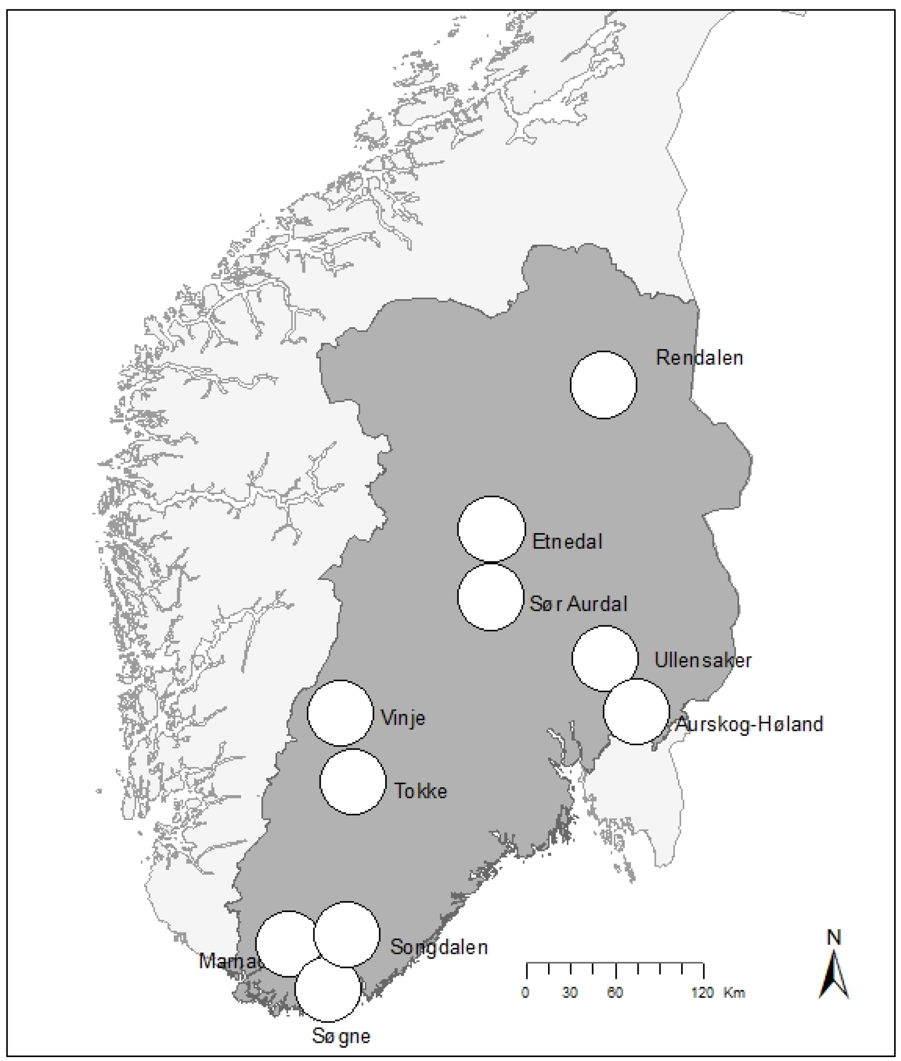
| Municipality | Investigated Area (km2) | Area of CHI Habitat (km2) | Number of CHI Habitats | Lowest Altitude (masl) | Highest Altitude (masl) |
|---|---|---|---|---|---|
| Aurskog-Høland | 619 | 12 | 1023 | 111 | 391 |
| Ullensaker | 103 | 1 | 84 | 114 | 302 |
| Marnardal | 293 | 4 | 1364 | 17 | 502 |
| Songdalen | 152 | 5 | 930 | 0 | 405 |
| Søgne | 103 | 3 | 1068 | 0 | 263 |
| Etnedal | 259 | 5 | 733 | 213 | 1024 |
| Sør-Aurdal | 618 | 15 | 1518 | 153 | 1034 |
| Tokke | 280 | 15 | 1538 | 12 | 958 |
| Rendalen | 299 | 7 | 618 | 232 | 941 |
| Vinje | 208 | 14 | 594 | 183 | 968 |
| Sum | 2934 | 81 | 9470 |
2.2. Analyses
3. Results
3.1. Spatial Clustering
| Distance (km) | ||||||||
|---|---|---|---|---|---|---|---|---|
| Habitat | 0–1.0 | 1.1–2.0 | 2.1–3.0 | 3.1–4.0 | 4.1–5.0 | 5.1–6.0 | 6.1–7.0 | 7.1–8.0 |
| Logs | 9/10 | 9/10 | 8/10 | 8/9 | 6/7 | 4/5 | 3/4 | 1/2 |
| Late succ | 10/10 | 9/10 | 7/10 | 7/9 | 5/8 | 3/3 | 2/2 | 2/2 |
| Old trees | 8/9 | 8/9 | 8/9 | 5/8 | 4/6 | 2/5 | 2/4 | 1/3 |
| Lux ground | 10/10 | 9/10 | 8/10 | 7/9 | 6/8 | 4/6 | 1/4 | 0/1 |
| Rich bark | 8/8 | 5/8 | 4/8 | 3/6 | 3/4 | 1/2 | 0/1 | - |
| Sum | 0.96 | 0.85 | 0.74 | 0.73 | 0.73 | 0.67 | 0.53 | 0.50 |
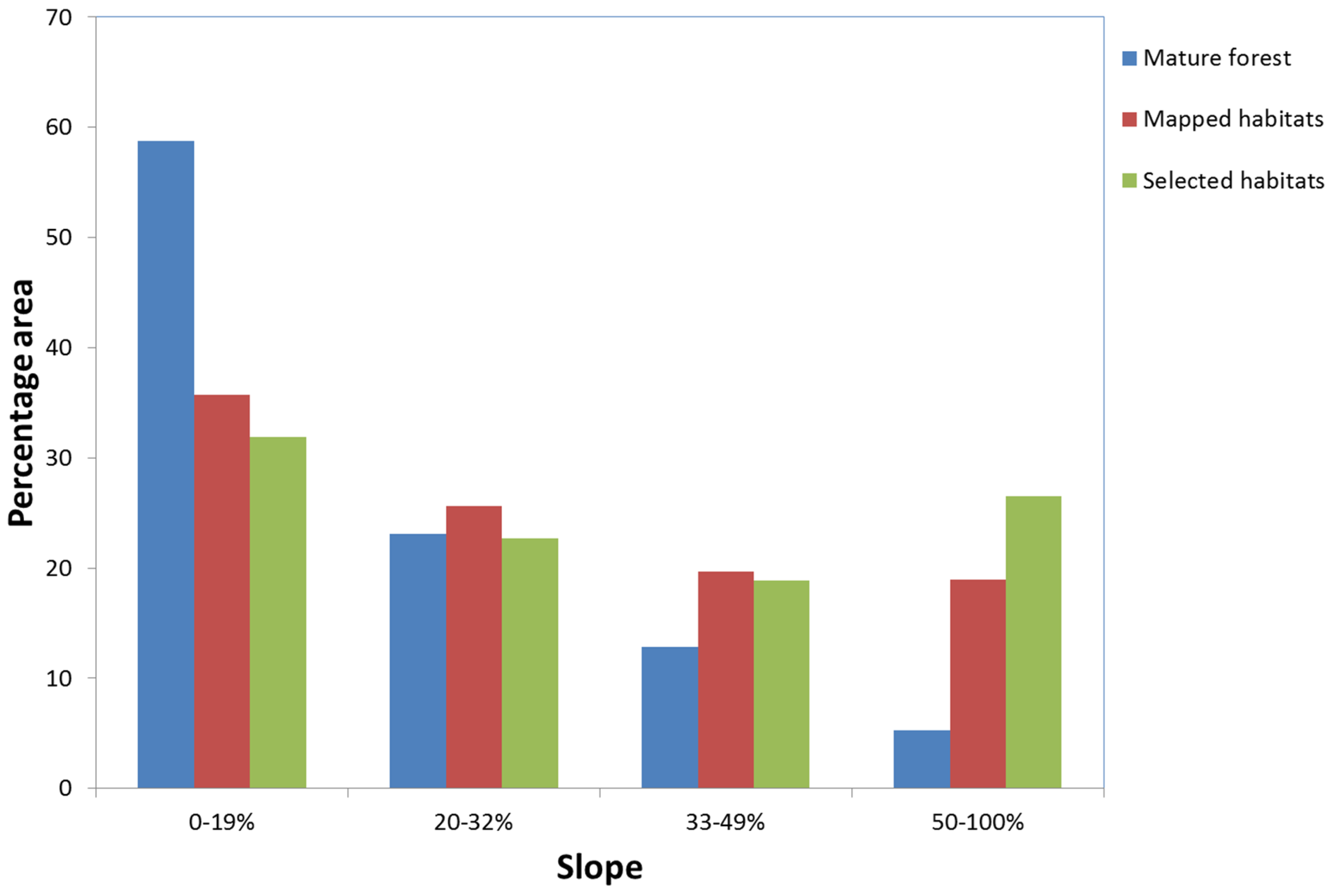
3.2. Slope
| CHI hab | Slope | Site Index | Altitude | Distance from Road | ||||||||
|---|---|---|---|---|---|---|---|---|---|---|---|---|
| Flatter | NS | Steeper | Lower | NS | Higher | Lower | NS | Higher | Shorter | NS | Longer | |
| All Forest | ||||||||||||
| Snags | 1 | 0 | 3 | 0 | 3 | 1 | 0 | 3 | 1 | 0 | 2 | 2 |
| Logs | 0 | 1 | 9 | 0 | 1 | 9 | 6 | 2 | 2 | 0 | 0 | 10 |
| Late succ | 0 | 3 | 7 | 0 | 0 | 10 | 7 | 2 | 1 | 3 | 6 | 1 |
| Pend lichen | 1 | 2 | 0 | 1 | 2 | 0 | 0 | 1 | 2 | 0 | 0 | 3 |
| Old trees | 0 | 2 | 7 | 5 | 0 | 4 | 2 | 0 | 7 | 0 | 2 | 7 |
| Lux ground | 0 | 2 | 8 | 0 | 0 | 10 | 9 | 0 | 1 | 3 | 6 | 1 |
| Rich bark | 0 | 1 | 6 | 0 | 2 | 5 | 4 | 3 | 0 | 0 | 7 | 0 |
| Total | 2 | 11 | 40 | 6 | 8 | 39 | 28 | 11 | 14 | 6 | 23 | 24 |
| Mature Forest | ||||||||||||
| Snags | 0 | 3 | 1 | 0 | 1 | 3 | 1 | 2 | 1 | 0 | 3 | 1 |
| Logs | 0 | 1 | 9 | 0 | 1 | 9 | 6 | 3 | 1 | 1 | 3 | 6 |
| Late succ | 0 | 3 | 6 | 0 | 0 | 9 | 7 | 1 | 1 | 5 | 4 | 0 |
| Pend lichen | 0 | 3 | 0 | 0 | 3 | 0 | 0 | 3 | 0 | 0 | 1 | 2 |
| Old trees | 0 | 2 | 7 | 4 | 1 | 4 | 2 | 3 | 4 | 1 | 2 | 6 |
| Lux ground | 0 | 2 | 8 | 0 | 1 | 9 | 7 | 3 | 0 | 5 | 4 | 1 |
| Rich bark | 0 | 2 | 4 | 0 | 2 | 4 | 3 | 3 | 0 | 1 | 5 | 0 |
| Total | 0 | 16 | 35 | 4 | 9 | 38 | 26 | 18 | 7 | 13 | 22 | 16 |
3.3. Site Index
3.4. Altitude
3.5. Distance from Road
4. Discussion
4.1. Habitat Distribution Patterns
4.2. Environmental Factors
4.3. The Impact of Forestry
4.4. Management Considerations

| Habitat | All forest Investigated | Steep Slopes | Low Altitudes | High Site Index | Long Distance from Road |
|---|---|---|---|---|---|
| Logs | 0.85 | 2.01 (2.36) | 1.43 (1.68) | 2.08 (2.45) | 0.88 (1.03) |
| Late succ | 0.31 | 0.66 (2.14) | 0.64 (2.05) | 0.91 (2.93) | 0.20 (0.63) |
| Old trees | 1.42 | 2.50 (1.76) | 0.87 (0.61) | 1.08 (0.76) | 2.83 (1.99) |
| Lux ground | 1.19 | 3.19 (2.68) | 3.12 (2.62) | 4.08 (3.43) | 0.56 (0.47) |
| Rich bark | 0.12 | 0.36 (3.02) | 0.32 (2.65) | 0.35 (2.92) | 0.08 (0.66) |
Supplementary Files
Supplementary File 1Acknowledgments
Author Contributions
Conflicts of Interest
References
- FAO. Global Forest Resources Assessment 2010. In FAO Forestry Paper; Food and Agricultural Organisation of the United Nations: Rome, Italy, 2010. [Google Scholar]
- CPF. Strategic Framework for Forests and Climate Change. In A proposal by the Collaborative Partnership on Forests for a Coordinated Forest-sector Response to Climate Change; The Collaborative Partnership on Forests: Bali, Indonesia, 2008. [Google Scholar]
- Lindenmayer, D.B.; Franklin, J.F.; Lõhmus, A.; Baker, S.C.; Bauhus, J.; Beese, W.; Brodie, A.; Kiehl, B.; Kouki, J.; Pasture, G.M.; et al. A major shift to the retention approach for forestry can help resolve some global forest sustainability issues. Cons. Lett. 2012, 5, 421–431. [Google Scholar] [CrossRef]
- Grau, O.; Grytnes, J.-A.; Birks, H.J.B. A comparison of altitudinal species richness patterns of bryophytes with other plant groups in Nepal, Central Himalaya. J. Biogeogr. 2007, 34, 1907–1915. [Google Scholar] [CrossRef]
- Rahbek, C. The role of spatial scale and the perception of large-scale species-richness patterns. Ecol. Lett. 2005, 8, 224–239. [Google Scholar] [CrossRef]
- Körner, C. Mountain biodiversity, its causes and function: An overview. In Mountain Biodiversity: A Global Assessment; Körner, C., Spehn, E.M., Eds.; Parthenon: Boca Raton, FL, USA, 2002; pp. 3–20. [Google Scholar]
- Grytnes, J.-A.; Heegaard, E.; Ihlen, P.G. Species richness of vascular plants, bryophytes, and lichens along an altitudinal gradient in western Norway. Acta Oecol. Int. J. Ecol. 2006, 29, 241–246. [Google Scholar] [CrossRef]
- Field, R.; Hawkins, B.A.; Cornell, H.V.; Currie, D.J.; Diniz-Filho, J.A.F.; Guegan, J.-F.; Kaufman, D.M.; Kerr, J.T.; Mittelbach, G.G.; Oberdorff, T.; et al. Spatial species-richness gradients across scales: A meta-analysis. J. Biogeogr. 2009, 36, 132–147. [Google Scholar] [CrossRef]
- Whittaker, R.J.; Willis, K.J.; Field, R. Scale and species richness: Towards a general hierarchical theory of species diversity. J. Biogeogr. 2001, 28, 453–470. [Google Scholar] [CrossRef]
- Gjerde, I.; Sætersdal, M.; Rolstad, J.; Storaunet, K.O.; Blom, H.H.; Gundersen, V.; Heegaard, E. Productivity-diversity relationships for plants, bryophytes, lichens, and polypore fungi in six northern forest landscapes. Ecography 2005, 28, 705–720. [Google Scholar] [CrossRef]
- Connell, J.H. Diversity in tropical rain forests and coral reefs: High diversity of trees and corals is maintained only in a non-equilibrium state. Science 1978, 199, 1302–1310. [Google Scholar] [CrossRef] [PubMed]
- Lindenmayer, D.B.; Franklin, J.F. Conserving Forest Biodiversity; Island Press: Washington, DC, USA, 2002. [Google Scholar]
- Franklin, J.F.; Berg, D.E.; Thornburgh, D.A.; Tappeiner, J.C. Alternative silvicultural approaches to timber harvest: Variable retention harvest systems. In Creating a Forestry for the 21st Century; Kohm, K.A., Franklin, J.F., Eds.; Island Press: Covelo, CA, USA, 1997; pp. 111–139. [Google Scholar]
- Timonen, J.; Siitonen, J.; Gustafsson, L.; Kotiaho, J.S.; Stokland, J.N.; Sverdrup-Thygeson, A.; Mönkkönen, M. Woodland key habitats in northern Europe: Concepts, inventory and protection. Scand. J. For. Res. 2010, 25, 309–324. [Google Scholar] [CrossRef]
- Granhus, A.; Hylen, G.; Nilsen, J.-E. Statistics of forest conditions and resources in Norway. Ressursoversikt fra Skog og Landskap 2012, 3, 1–85. [Google Scholar]
- Gjerde, I.; Sætersdal, M.; Blom, H.H. Complementary Hotspot Inventory—A method for identification of important areas for biodiversity at the forest stand level. Biol. Conserv. 2007, 137, 549–557. [Google Scholar] [CrossRef]
- Moen, A. National Atlas of Norway: Vegetation; Norwegian Mapping Authority: Hønefoss, Norway, 1999. [Google Scholar]
- ESRI. ArcMap: Release 10.0; Environmental Systems Research Institute: Redlands, CA, USA, 2013. [Google Scholar]
- Tveite, B.; Braastad, H. Bonitering av gran, furu og bjørk. Nor. Skogbr. 1981, 27, 17–22. [Google Scholar]
- Cressie, N.A.C. Statistics for Spatial Data Revised Edition; Wiley Series in Probability and Mathematical Statistics; John Wiley & Sons: New York, NY, USA, 1993. [Google Scholar]
- Gelman, A.; Carlin, J.; Stern, H.; Dunson, D.; Vehtari, A.; Rubin, D. Bayesian Data Analysis, 3rd ed.; Chapman & Hall: London, UK, 2013. [Google Scholar]
- Rue, H.; Martino, S.; Chopin, N. Bayesian inference for latent Gaussian models by using integrated nested Laplace approximations. J. R. Stat. Soc. 2009, 71, 319–392. [Google Scholar] [CrossRef]
- Blangiardo, M.; Cameletti, M. Spatial and Spatio-Temporal Bayesian Models with R—INLA; John Wiley & Sons: Chichester, UK, 2015. [Google Scholar]
- R Core Team. R: A Language and Environment for Statistical Computing, Rversion 3.1.1.; R Foundation for Statistical Computing: Vienna, Austria, 2014. [Google Scholar]
- Worrell, R. Damage by the spruce bark beetle in South Norway 1970–80: A survey, and factors affecting its occurrence. Rep. Nor. For. Res. Inst. 1983, 38, 1–34. [Google Scholar]
- Grant, R.F. Modeling topographic effects on net ecosystem productivity of boreal black spruce forests. Tree Physiol. 2004, 24, 1–18. [Google Scholar] [CrossRef] [PubMed]
- Laamrani, A.; Valeria, O.; Bergeron, Y.; Fenton, N.; Cheng, L.Z.; Anyomi, K. Effects of topography and thickness of organic layer on productivity of black spruce boreal forests of the Canadian Clay Belt region. For. Ecol. Manag. 2014, 330, 144–157. [Google Scholar] [CrossRef]
- Anyomi, K.; Raulier, F.; Girardin, M.; Bergeron, Y. Using height growth to model local and regional response of trembling aspen (Populus tremuloides Michx.) to climate within the boreal forest of western Quebec. Ecol. Mod. 2012, 243, 123–132. [Google Scholar] [CrossRef]
- Laaksonen, K. Areal distribution of monthly mean air temperatures in Fennoscandia (1921–1950). Fennia 1979, 157, 89–124. [Google Scholar]
- Storaunet, K.O.; Rolstad, J.; Gjerde, I.; Gundersen, V.S. Historical logging, productivity, and structural characteristics of boreal coniferous forests in Norway. Silva Fenn. 2005, 39, 429–442. [Google Scholar] [CrossRef]
- Sippola, A.-L.; Siitonen, J.; Kallio, R. Amount and quality of coarse woody debris in natural and managed coniferous forests near the timberline in Finnish Lapland. Scand. J. For. Res. 1998, 13, 204–214. [Google Scholar] [CrossRef]
- Johnson, B.G.; Abrams, M.D. Age class, longevity and growth rate relationships: Protracted growth increases in old trees in eastern United States. Tree Physiol. 2009, 29, 1317–1328. [Google Scholar] [CrossRef] [PubMed]
- Stokland, J.N.; Larsson, K.-H. Legacies from natural forest dynamics: Different effects of forest management on wood-inhabiting fungi in pine and spruce forests. For. Ecol. Manag. 2011, 261, 1707–1721. [Google Scholar] [CrossRef]
- Braathe, P. The background of the transition to forest stand management. Tidsskr. Skogbruk 1980, 88, 143–148. [Google Scholar]
- Jonsson, B.G.; Hofgaard, A. The structure and regeneration of high-altitude Norway spruce forests: A review of Arnborg (1942, 1943). Scand. J. For. Res. 2011, 26, 17–24. [Google Scholar] [CrossRef]
- Sverdrup-Thygeson, A.; Bendiksen, E.; Birkemoe, T.; Larsson, K.H. Do conservation measures in forest work? A comparison of three area-based conservation tools for wood-living species in boreal forests. For. Ecol. Manag. 2014, 330, 8–16. [Google Scholar] [CrossRef]
- Wikberg, S.; Perhans, K.; Kindstrand, C.; Djupström, L.B.; Boman, M.; Mattson, L.; Schroeder, L.M.; Weslien, J.; Gustafsson, L. Cost-effectiveness of conservation strategies implemented in boreal forests: The area selection process. Biol. Cons. 2009, 142, 614–624. [Google Scholar] [CrossRef]
- Søvde, N.E.; Sætersdal, M.; Løkketangen, A. A scenario-based method for assessing the impact of suggested woodland key habitats on forest harvesting costs. Forests 2014, 5, 2327–2344. [Google Scholar] [CrossRef]
- Næsset, E. Airborne laser scanning as a method in operational forest inventory: Status of accuracy assessments accomplished in Scandinavia. Scand. J. For. Res. 2007, 22, 433–442. [Google Scholar] [CrossRef]
© 2016 by the authors; licensee MDPI, Basel, Switzerland. This article is an open access article distributed under the terms and conditions of the Creative Commons by Attribution (CC-BY) license (http://creativecommons.org/licenses/by/4.0/).
Share and Cite
Sætersdal, M.; Gjerde, I.; Heegaard, E.; Schei, F.H.; Nilsen, J.E.Ø. History and Productivity Determine the Spatial Distribution of Key Habitats for Biodiversity in Norwegian Forest Landscapes. Forests 2016, 7, 11. https://doi.org/10.3390/f7010011
Sætersdal M, Gjerde I, Heegaard E, Schei FH, Nilsen JEØ. History and Productivity Determine the Spatial Distribution of Key Habitats for Biodiversity in Norwegian Forest Landscapes. Forests. 2016; 7(1):11. https://doi.org/10.3390/f7010011
Chicago/Turabian StyleSætersdal, Magne, Ivar Gjerde, Einar Heegaard, Fride Høistad Schei, and Jan Erik Ørnelund Nilsen. 2016. "History and Productivity Determine the Spatial Distribution of Key Habitats for Biodiversity in Norwegian Forest Landscapes" Forests 7, no. 1: 11. https://doi.org/10.3390/f7010011
APA StyleSætersdal, M., Gjerde, I., Heegaard, E., Schei, F. H., & Nilsen, J. E. Ø. (2016). History and Productivity Determine the Spatial Distribution of Key Habitats for Biodiversity in Norwegian Forest Landscapes. Forests, 7(1), 11. https://doi.org/10.3390/f7010011