Juvenile Southern Pine Response to Fertilization Is Influenced by Soil Drainage and Texture

Abstract

We examined three hypotheses in a nutrient dose and application frequency study installed in juvenile (aged 2–6 years old) Pinus stands at 22 sites in the southeastern United States. At each site, eight or nine treatments were installed where nitrogen was applied at different rates (0, 67, 134, 268 kg ha⁻¹) and frequencies (0, 1, 2, 4 and 6 years) in two or four replications. Phosphorus was applied at 0.1 times the nitrogen rate and other elements were added as needed based on foliar nutrient analysis to insure that nutrient imbalances were not induced with treatment. Eight years after treatment initiation, the site responses were grouped based on texture and drainage characteristics: soil group 1 consisted of poorly drained soils with a clayey subsoil, group 2 consisted of poorly to excessively drained spodic soils or soils without a clay subsoil, and group 3 consisted of well-drained soils with a clayey subsoil. We accepted the first hypothesis that site would be a significant factor explaining growth responses. Soil group was also a significant factor explaining growth response. We accepted our second hypothesis that the volume growth-cumulative dose response function was not linear. Volume growth reached an asymptote in soil groups 1 and 3 between cumulative nitrogen doses of 300–400 kg ha⁻¹. Volume growth responses continued to increase up to 800 kg ha⁻¹ of cumulatively applied nitrogen for soil group 2. We accepted our third hypothesis that application rate and frequency did not influence the growth response when the cumulative nitrogen dose was equivalent. There was no difference in the growth response for comparisons where a cumulative nitrogen dose of 568 kg ha⁻¹ was applied as 134 kg ha⁻¹ every two years or as 269 kg ha⁻¹ every four years, or where 269 kg ha⁻¹ of nitrogen was applied as four applications of 67 kg ha⁻¹ every two years or as two applications of 134 kg ha⁻¹ every four years. Clearly, the sites examined here were limited by nitrogen and phosphorus, and applications of these elements to young stands effectively ameliorated these limitations. However, there were differences in the response magnitude that were related to soil texture and drainage. Juvenile fertilizer applications resulted in high stocking levels early in the rotation; this condition should be considered when undertaking juvenile fertilization programs.

1. Introduction

Light interception drives the growth of forest plantations [1,2,3]. In the southeast United States, the primary commercial tree species are Pinus taeda L. and P. elliottii Engelm. which account for 16% of the world’s timber production [4]. Theoretical estimates of light interception and productivity indicate that a maximum leaf area index of approximately 4 [5,6] is possible in southeast US pine stands, but stands often fall short of this level primarily due to nitrogen and phosphorus limitations observed at mid-rotation [7,8,9]. Empirical trials have identified an average response of 3.5 m³ ha⁻¹ yr⁻¹ over an eight-year period to the application of 224 and 28 kg ha⁻¹ of elemental nitrogen and phosphorus, respectively, in mid-rotation stands across a wide range of sites [10].

Early in the rotation, nitrogen and phosphorus are typically more readily available from mineralization of the litter layer from the previous rotation. This effect, known as the assart effect [11,12], likely dissipates and nitrogen availability returns to background levels within five years [13]. In studies where the forest floor was manipulated (doubled in some plots, removed in other plots), improved nitrogen availability was found through age 10 [14]. Similarly, silvicultural treatments such as intensive site preparation, vegetation control and fertilization applied at planting may result in large growth gains and increased leaf area through age 10 [15,16]. However, in typical stands, the assart effect and effects from early rotation or time of planting treatments would likely be diminished before a midrotation fertilizer treatment would be applied (8–10 years of age) [17]. Once leaf area levels are reduced through a lack of resources, it may take up to three years to build the crown back up to a high level of leaf area [18]. Given these conditions, it is likely that the productive potential of many sites may not be achieved without the application of additional resources (nitrogen and phosphorus, in this case) prior to midrotation.

The midrotation application of 224 and 28 kg ha⁻¹ of elemental nitrogen and phosphorus, respectively, has resulted in a positive growth response in 85% of research trials with a range in response from 0.7 to 7.0 m³ ha⁻¹ yr⁻¹ over an eight-year period [19]. However, the growth response reaches a peak between two and four years after treatment application [20]. Whereas the growth response was linearly related to the amount of nitrogen applied (up to 336 kg ha⁻¹), the growth response per unit of applied nitrogen was higher at lower doses [20]. At a conceptual and practical level, applying nutrients when and in the amounts needed by plants has resulted in near 100% uptake of applied nutrients in laboratory and field experiments [21,22,23]. In this framework there may be benefit to applying nutrients in lower doses more frequently. Consequently, there is uncertainty about the appropriate dose and frequency of application if one were to consider ameliorating potential nutrient limitations in juvenile stands.

Given these circumstances, our interest was in quantifying juvenile pine plantation response to nutrient additions. If a difference in response to treatment was observed across sites, we wanted to identify site-soil variables that would help group the responses patterns. We wanted to determine the shape of the growth response curve especially at nutrient applications greater than 336 kg nitrogen ha⁻¹ and how best to apply nutrients (low, frequent doses or larger, less frequent doses). Specifically, we tested the following hypotheses: site would influence juvenile plantation response to nitrogen and phosphorus additions (there would be a site effect), the relationship between volume growth response and applied nitrogen would not be linear (there is a maximum amount of applied nitrogen beyond which growth improvements would be small and other resources would become limiting) and the overall applied nitrogen dose and not the application frequency would determine the growth response (e.g. the growth response from 538 kg ha⁻¹ nitrogen would be the same whether the nitrogen was applied in two doses of 269 or four doses of 134 kg ha⁻¹ nitrogen).

2. Materials and Methods

Twenty-two sites were selected to represent a range of soil, physiography, geology and drainage conditions in the southeastern United States (Table 1 and Table 2). Selected sites were well stocked, growing vigorously and had minimal woody competition. Silvicultural practices used to create these conditions varied by site and included tillage (poorly drained sites were typically bedded), chemical site preparation (typical for upland sites), herbaceous vegetation control (common on most sites) and fertilization (phosphorus was applied on phosphorus deficient sites). Vegetation control was not included in our treatments, at treatment initiation planted pines had already captured or were poised to capture the site in most cases. Stand age at treatment initiation ranged from two to six years. Installation occurred from 1998 to 2003. Selected sites were assigned to a Cooperative Research in Forest Fertilization (CRIFF) program soils group based on their drainage and subsurface soil texture [24] (Table 2). All sites were cutover natural pine stands or plantations. Site 22 was planted to P. elliottii and all other sites were planted to P. taeda. Prior to treatment initiation, stocking across all sites ranged from 1216 to 2246 trees ha⁻¹, diameter at breast height ranged from 0.9 to 10.2 cm, height ranged from 1.4 to 7.2 m, basal area ranged from 0.1 to 13.5 m² ha⁻¹ and stem volume ranged from 5.3 to 49.6 m³ ha⁻¹ (Table 3).

Table 1. Location, age and year of study initiation for the sites examined in this study.

Site	County	State	Latitude (decimal degrees)	Longitude (decimal degrees)	Year of Initiation (year)	Age at Initiation (years)
1	Kershaw	SC	34.45	−80.50	2000	4
2	Oglethorpe	GA	33.89	−82.91	2000	6
3	Brunswick	VA	36.68	−77.99	1999	6
4	Berkeley	SC	33.19	−80.19	1999	5
5	Coosa	AL	32.91	−86.38	2002	6
6	Floyd	GA	34.15	−85.38	2001	3
7	Angelina	TX	31.13	−94.46	2003	3
8	Wilkes	GA	33.81	−82.96	2000	3
9	Nassau	FL	30.68	−81.75	1999	5
10	Sabine	LA	31.72	−93.56	1999	5
11	Vernon	LA	31.34	−93.18	2000	6
12	Marengo	AL	32.37	−87.84	2001	3
13	Brantley	GA	31.34	−81.82	1998	3
14	Brantley	GA	31.34	−81.83	1998	2
15	Marion	GA	32.17	−84.63	2000	4
16	Talbot	GA	32.68	−84.74	2003	5
17	Bradley	AR	33.49	−92.13	2000	5
18	Marengo	AL	32.25	−87.55	2000	4
19	Newton	TX	30.48	−93.78	2001	2
20	Montgomery	NC	35.28	−79.94	2003	4
21	Montgomery	MS	32.55	−89.64	2003	6
22	Dixie	FL	29.65	−83.17	2003	3

Table 1. Location, age and year of study initiation for the sites examined in this study.

Site	County	State	Latitude (decimal degrees)	Longitude (decimal degrees)	Year of Initiation (year)	Age at Initiation (years)
1	Kershaw	SC	34.45	−80.50	2000	4
2	Oglethorpe	GA	33.89	−82.91	2000	6
3	Brunswick	VA	36.68	−77.99	1999	6
4	Berkeley	SC	33.19	−80.19	1999	5
5	Coosa	AL	32.91	−86.38	2002	6
6	Floyd	GA	34.15	−85.38	2001	3
7	Angelina	TX	31.13	−94.46	2003	3
8	Wilkes	GA	33.81	−82.96	2000	3
9	Nassau	FL	30.68	−81.75	1999	5
10	Sabine	LA	31.72	−93.56	1999	5
11	Vernon	LA	31.34	−93.18	2000	6
12	Marengo	AL	32.37	−87.84	2001	3
13	Brantley	GA	31.34	−81.82	1998	3
14	Brantley	GA	31.34	−81.83	1998	2
15	Marion	GA	32.17	−84.63	2000	4
16	Talbot	GA	32.68	−84.74	2003	5
17	Bradley	AR	33.49	−92.13	2000	5
18	Marengo	AL	32.25	−87.55	2000	4
19	Newton	TX	30.48	−93.78	2001	2
20	Montgomery	NC	35.28	−79.94	2003	4
21	Montgomery	MS	32.55	−89.64	2003	6
22	Dixie	FL	29.65	−83.17	2003	3

Table 2. Soils, physiography and geology for the sites examined in this study. Cooperative Research in Forest Fertilization (CRIFF) program soils groups are based on drainage and subsurface texture where groups A and B are poorly drained with clay subsurface, C and G are poorly to well drained with no clay in the subsurface and E and F are well drained with a clay subsurface. The current study soil group combines CRIFF A and B soils (current study group 1), CRIFF C and G soils (current study group 2) and CRIFF E and F soils (current study group 3).

site	CRIFF Soils Group	Current study soil group	Physiographic Province	Soil Series	Drainage	Geologic formation	Soil taxonomy
1	G	2	Sandhills	Blanton	Well	Cretaceous, Upper, Lumbee, Black Creek	Typic Quartzipsamments
2	E	3	Piedmont	Iredell	Moderately well	Diabase Ultramafic	Fine, mixed, active, thermic Oxyaquic Vertic Hapludalfs
3	E	3	Piedmont	Cecil	Well	Biotite Gneiss	Fine, Kaolinitic, Thermic Typic Kanhapludults
4	B	1	Atlantic Coastal Plain	Lynchburg	Somewhat poorly	Quaternary, Pleistocene, Penholoway	Fine-loamy, siliceous, semiactive, thermic Aeric Paleaquults
5	E	3	Piedmont	Louisa	Well	Biotite Gneiss	Loamy, Micaceous, Thermic, Shallow Typic Dystrudepts
6	E	3	Ridge and Valley	Townley	Moderately well	Conasauga Shale	Fine, Mixed, Semiactive, Thermic, Typic Hapludults
7	E	3	Upper Gulf Coastal Plain	Kurth	Moderately well	Tertiary, Eocene, Jackson, Manning	Fine-Loamy, siliceous, semiactive, thermic Oxyaquic Glossudalfs
8	E	3	Piedmont	Appling	Well	Metadacite	Fine, kaolinitic, thermic Typic Kanhapludults
9	A	1	Flatwoods	Meggett	Poorly	Quaternary, Pleistocene, Wicomico	Fine, Mixed, Active, Thermic, Typic Albaqualf
10	E	3	Upper Gulf Coastal Plain	Sacul	Moderately well	Tertiary, Paleocene, Wilcox, Undifferentiated	Fine, mixed, active, thermic aquic hapludults
11	A	1	Lower Gulf Coastal Plain	Mayhew	Somewhat poorly	Tertiary, Miocene, Fleming, Carnahan Bayou	Fine, smectitic, thermic Chromic Dystraquerts
12	A	1	Upper Gulf Coastal Plain	Lenoir	Somewhat poorly	Quaternary, Holocene, High Terrace	Fine, mixed, semiactive, thermic Aeric Paleaquults
13	C	2	Flatwoods	Seagate	Somewhat poorly	Quaternary, Pleistocene, Penholoway	Sandy over loamy, Siliceous, Active, Thermic Typic Haplohumods
14	C	2	Flatwoods	Pelham	Poorly	Quaternary, Pleistocene, Penholoway	Loamy, Siliceous, Subactive, Thermic Arenic Paleaquults
15	F	3	Lower Gulf Coastal Plain	Troup	Well	Cretaceous, Upper, Navarro, Providence	Loamy, Kaolinitic, thermic Grossarenic Kandiudults
16	E	3	Piedmont	Cecil	Well	Gneiss	Fine, Kaolinitic, Thermic Typic Kanhapludults
17	B	1	Upper Gulf Coastal Plain	Stough	Somewhat poorly	Quaternary, Pleistocene, High Terrace	Coarse, Loamy, Siliceous, Thermic Fragiaquic Paleudults
18	A	1	Upper Gulf Coastal Plain	Brantley	Well	Cretaceous, Upper, Taylor, Ripley	Fine, Mixed active, Thermic Ultic Haplidults
19	B	1	Lower Gulf Coastal Plain	Evadale	Poorly	Quaternary, Pleistocene, Beaumont	Fine Smectitic, Thermic Typic glossaqualfs
20	E	3	Piedmont	Herndon	Well	Carolina Slate	Fine, kaolinitic, thermic Typic Kanhapludults
21	B	1	Upper Gulf Coastal Plain	Shabuta	Well	Tertiary, Eocene, Claiborne, Cook Mountain	Fine, mixed, semiactive, thermic Typic Paleudults
22	C	2	Flatwoods	Sapelo	Somewhat poorly	Tertiary, Eocene, Ocala Limestone	Sandy, siliceous, thermic Ultic Alaquods

Table 2. Soils, physiography and geology for the sites examined in this study. Cooperative Research in Forest Fertilization (CRIFF) program soils groups are based on drainage and subsurface texture where groups A and B are poorly drained with clay subsurface, C and G are poorly to well drained with no clay in the subsurface and E and F are well drained with a clay subsurface. The current study soil group combines CRIFF A and B soils (current study group 1), CRIFF C and G soils (current study group 2) and CRIFF E and F soils (current study group 3).

site	CRIFF Soils Group	Current study soil group	Physiographic Province	Soil Series	Drainage	Geologic formation	Soil taxonomy
1	G	2	Sandhills	Blanton	Well	Cretaceous, Upper, Lumbee, Black Creek	Typic Quartzipsamments
2	E	3	Piedmont	Iredell	Moderately well	Diabase Ultramafic	Fine, mixed, active, thermic Oxyaquic Vertic Hapludalfs
3	E	3	Piedmont	Cecil	Well	Biotite Gneiss	Fine, Kaolinitic, Thermic Typic Kanhapludults
4	B	1	Atlantic Coastal Plain	Lynchburg	Somewhat poorly	Quaternary, Pleistocene, Penholoway	Fine-loamy, siliceous, semiactive, thermic Aeric Paleaquults
5	E	3	Piedmont	Louisa	Well	Biotite Gneiss	Loamy, Micaceous, Thermic, Shallow Typic Dystrudepts
6	E	3	Ridge and Valley	Townley	Moderately well	Conasauga Shale	Fine, Mixed, Semiactive, Thermic, Typic Hapludults
7	E	3	Upper Gulf Coastal Plain	Kurth	Moderately well	Tertiary, Eocene, Jackson, Manning	Fine-Loamy, siliceous, semiactive, thermic Oxyaquic Glossudalfs
8	E	3	Piedmont	Appling	Well	Metadacite	Fine, kaolinitic, thermic Typic Kanhapludults
9	A	1	Flatwoods	Meggett	Poorly	Quaternary, Pleistocene, Wicomico	Fine, Mixed, Active, Thermic, Typic Albaqualf
10	E	3	Upper Gulf Coastal Plain	Sacul	Moderately well	Tertiary, Paleocene, Wilcox, Undifferentiated	Fine, mixed, active, thermic aquic hapludults
11	A	1	Lower Gulf Coastal Plain	Mayhew	Somewhat poorly	Tertiary, Miocene, Fleming, Carnahan Bayou	Fine, smectitic, thermic Chromic Dystraquerts
12	A	1	Upper Gulf Coastal Plain	Lenoir	Somewhat poorly	Quaternary, Holocene, High Terrace	Fine, mixed, semiactive, thermic Aeric Paleaquults
13	C	2	Flatwoods	Seagate	Somewhat poorly	Quaternary, Pleistocene, Penholoway	Sandy over loamy, Siliceous, Active, Thermic Typic Haplohumods
14	C	2	Flatwoods	Pelham	Poorly	Quaternary, Pleistocene, Penholoway	Loamy, Siliceous, Subactive, Thermic Arenic Paleaquults
15	F	3	Lower Gulf Coastal Plain	Troup	Well	Cretaceous, Upper, Navarro, Providence	Loamy, Kaolinitic, thermic Grossarenic Kandiudults
16	E	3	Piedmont	Cecil	Well	Gneiss	Fine, Kaolinitic, Thermic Typic Kanhapludults
17	B	1	Upper Gulf Coastal Plain	Stough	Somewhat poorly	Quaternary, Pleistocene, High Terrace	Coarse, Loamy, Siliceous, Thermic Fragiaquic Paleudults
18	A	1	Upper Gulf Coastal Plain	Brantley	Well	Cretaceous, Upper, Taylor, Ripley	Fine, Mixed active, Thermic Ultic Haplidults
19	B	1	Lower Gulf Coastal Plain	Evadale	Poorly	Quaternary, Pleistocene, Beaumont	Fine Smectitic, Thermic Typic glossaqualfs
20	E	3	Piedmont	Herndon	Well	Carolina Slate	Fine, kaolinitic, thermic Typic Kanhapludults
21	B	1	Upper Gulf Coastal Plain	Shabuta	Well	Tertiary, Eocene, Claiborne, Cook Mountain	Fine, mixed, semiactive, thermic Typic Paleudults
22	C	2	Flatwoods	Sapelo	Somewhat poorly	Tertiary, Eocene, Ocala Limestone	Sandy, siliceous, thermic Ultic Alaquods

Table 3. Tree and stand measurements (diameter at breast height, height, basal area, volume and stocking) and foliar nutrient concentration (nitrogen, phosphorus, potassium, calcium, and magnesium) mean and standard deviation (SE) prior to treatment initiation for the 22 sites where fertilizers were applied in varying doses and frequencies. Diameter at breast height was not measured at Site 14 prior to treatment initiation.

Current study soil group	Site	Diameter		Height		Basal area		Volume		Stocking		Nitrogen		Phosphorus		Potassium		Calcium		Magnesium
		Mean	SE	mean	SE	mean	SE	mean	SE	mean	SE	mean	SE	mean	SE	mean	SE	mean	SE	mean	SE
		(cm)		(m)		(m2 ha−1)		(m3 ha−1)		(trees ha−1)		(%)		(%)		(%)		(%)		(%)
1	4	10.2	0.1	7.2	0.0	13.5	0.2	49.6	1.8	1,591	18	1.19	0.01	0.14	0.00	0.40	0.01	0.18	0.00	0.10	0.00
1	9	7.7	0.1	5.1	0.1	11.2	0.3	40.6	1.1	2,246	24	1.18	0.02	0.11	0.00	0.39	0.01	0.31	0.01	0.15	0.00
1	11	7.6	0.1	5.9	0.1	8.3	0.2	33.2	1.0	1,731	54	0.95	0.01	0.08	0.00	0.38	0.01	0.17	0.01	0.08	0.00
1	12	4.4	0.1	3.8	0.0	2.4	0.1	13.0	0.2	1,412	17	0.99	0.02	0.11	0.00	0.51	0.01	0.16	0.00	0.07	0.00
1	17	5.7	0.2	3.7	0.0	3.4	0.3	13.6	0.5	1,247	32	1.08	0.01	0.11	0.00	0.51	0.01	0.14	0.00	0.07	0.00
1	18	3.2	0.1	3.0	0.0	1.3	0.0	10.7	0.1	1,416	23	1.27	0.02	0.15	0.00	0.57	0.01	0.22	0.01	0.09	0.00
1	19	1.3	0.0	1.6	0.0	0.2	0.0	6.6	0.3	1,266	29	1.09	0.02	0.11	0.00	0.37	0.01	0.30	0.01	0.09	0.00
1	21	9.4	0.1	6.0	0.1	9.5	0.3	34.3	1.2	1,331	10	1.21	0.02	0.13	0.00	0.58	0.02	0.19	0.01	0.09	0.00
2	1	0.9	0.0	1.4	0.0	0.1	0.0	5.3	0.4	1,441	23	0.96	0.01	0.11	0.00	0.35	0.01	0.21	0.01	0.06	0.00
2	13	3.9	0.1	3.2	0.0	2.2	0.1	14.0	0.3	1,699	34	1.06	0.02	0.13	0.00	0.29	0.01	0.17	0.01	0.11	0.00
2	14			2.1	0.0					1,749	20	1.05	0.02	0.13	0.00	0.29	0.02	0.31	0.01	0.13	0.00
2	22	3.8	0.1	2.9	0.0	1.9	0.1	12.2	0.2	1,576	31	0.64	0.01	0.06	0.00	0.26	0.01	0.21	0.01	0.10	0.00
3	2	5.9	0.1	3.5	0.0	4.7	0.2	17.8	0.5	1,635	36	1.14	0.01	0.11	0.00	0.44	0.01	0.23	0.01	0.12	0.00
3	3	7.3	0.1	4.8	0.0	7.3	0.2	26.4	0.5	1,678	24	1.20	0.01	0.11	0.00	0.53	0.01	0.19	0.01	0.07	0.00
3	5	8.1	0.2	5.8	0.1	7.9	0.3	29.9	0.9	1,458	19	1.22	0.02	0.11	0.00	0.43	0.01	0.20	0.01	0.09	0.00
3	6	3.5	0.0	3.0	0.0	1.7	0.0	12.6	0.1	1,655	13	1.01	0.02	0.11	0.00	0.49	0.01	0.17	0.01	0.05	0.00
3	7	4.2	0.1	3.1	0.1	1.9	0.1	10.7	0.3	1,268	29	1.15	0.03	0.12	0.01	0.57	0.05	0.26	0.02	0.09	0.01
3	8	1.5	0.0	2.1	0.0	0.4	0.0	11.1	0.2	1,817	23	1.26	0.01	0.12	0.00	0.54	0.01	0.25	0.01	0.10	0.00
3	10	7.4	0.1	4.9	0.0	9.4	0.3	34.3	0.8	2,125	42	1.30	0.02	0.10	0.00	0.59	0.01	0.14	0.00	0.09	0.00
3	15	2.7	0.0	2.7	0.0	1.2	0.0	12.3	0.1	1,725	14	1.13	0.03	0.13	0.00	0.42	0.02	0.21	0.01	0.09	0.00
3	16	8.2	0.1	5.8	0.0	7.2	0.1	27.0	0.5	1,315	21	1.21	0.01	0.11	0.00	0.42	0.01	0.29	0.00	0.12	0.00
3	20	5.3	0.1	3.3	0.0	2.9	0.1	12.0	0.3	1,216	25	1.32	0.02	0.12	0.00	0.59	0.01	0.16	0.01	0.06	0.00
Adequate nutrient concentration levels from [25]												1.20		0.12		0.35		0.15		0.08

Table 3. Tree and stand measurements (diameter at breast height, height, basal area, volume and stocking) and foliar nutrient concentration (nitrogen, phosphorus, potassium, calcium, and magnesium) mean and standard deviation (SE) prior to treatment initiation for the 22 sites where fertilizers were applied in varying doses and frequencies. Diameter at breast height was not measured at Site 14 prior to treatment initiation.

Current study soil group	Site	Diameter		Height		Basal area		Volume		Stocking		Nitrogen		Phosphorus		Potassium		Calcium		Magnesium
		Mean	SE	mean	SE	mean	SE	mean	SE	mean	SE	mean	SE	mean	SE	mean	SE	mean	SE	mean	SE
		(cm)		(m)		(m2 ha−1)		(m3 ha−1)		(trees ha−1)		(%)		(%)		(%)		(%)		(%)
1	4	10.2	0.1	7.2	0.0	13.5	0.2	49.6	1.8	1,591	18	1.19	0.01	0.14	0.00	0.40	0.01	0.18	0.00	0.10	0.00
1	9	7.7	0.1	5.1	0.1	11.2	0.3	40.6	1.1	2,246	24	1.18	0.02	0.11	0.00	0.39	0.01	0.31	0.01	0.15	0.00
1	11	7.6	0.1	5.9	0.1	8.3	0.2	33.2	1.0	1,731	54	0.95	0.01	0.08	0.00	0.38	0.01	0.17	0.01	0.08	0.00
1	12	4.4	0.1	3.8	0.0	2.4	0.1	13.0	0.2	1,412	17	0.99	0.02	0.11	0.00	0.51	0.01	0.16	0.00	0.07	0.00
1	17	5.7	0.2	3.7	0.0	3.4	0.3	13.6	0.5	1,247	32	1.08	0.01	0.11	0.00	0.51	0.01	0.14	0.00	0.07	0.00
1	18	3.2	0.1	3.0	0.0	1.3	0.0	10.7	0.1	1,416	23	1.27	0.02	0.15	0.00	0.57	0.01	0.22	0.01	0.09	0.00
1	19	1.3	0.0	1.6	0.0	0.2	0.0	6.6	0.3	1,266	29	1.09	0.02	0.11	0.00	0.37	0.01	0.30	0.01	0.09	0.00
1	21	9.4	0.1	6.0	0.1	9.5	0.3	34.3	1.2	1,331	10	1.21	0.02	0.13	0.00	0.58	0.02	0.19	0.01	0.09	0.00
2	1	0.9	0.0	1.4	0.0	0.1	0.0	5.3	0.4	1,441	23	0.96	0.01	0.11	0.00	0.35	0.01	0.21	0.01	0.06	0.00
2	13	3.9	0.1	3.2	0.0	2.2	0.1	14.0	0.3	1,699	34	1.06	0.02	0.13	0.00	0.29	0.01	0.17	0.01	0.11	0.00
2	14			2.1	0.0					1,749	20	1.05	0.02	0.13	0.00	0.29	0.02	0.31	0.01	0.13	0.00
2	22	3.8	0.1	2.9	0.0	1.9	0.1	12.2	0.2	1,576	31	0.64	0.01	0.06	0.00	0.26	0.01	0.21	0.01	0.10	0.00
3	2	5.9	0.1	3.5	0.0	4.7	0.2	17.8	0.5	1,635	36	1.14	0.01	0.11	0.00	0.44	0.01	0.23	0.01	0.12	0.00
3	3	7.3	0.1	4.8	0.0	7.3	0.2	26.4	0.5	1,678	24	1.20	0.01	0.11	0.00	0.53	0.01	0.19	0.01	0.07	0.00
3	5	8.1	0.2	5.8	0.1	7.9	0.3	29.9	0.9	1,458	19	1.22	0.02	0.11	0.00	0.43	0.01	0.20	0.01	0.09	0.00
3	6	3.5	0.0	3.0	0.0	1.7	0.0	12.6	0.1	1,655	13	1.01	0.02	0.11	0.00	0.49	0.01	0.17	0.01	0.05	0.00
3	7	4.2	0.1	3.1	0.1	1.9	0.1	10.7	0.3	1,268	29	1.15	0.03	0.12	0.01	0.57	0.05	0.26	0.02	0.09	0.01
3	8	1.5	0.0	2.1	0.0	0.4	0.0	11.1	0.2	1,817	23	1.26	0.01	0.12	0.00	0.54	0.01	0.25	0.01	0.10	0.00
3	10	7.4	0.1	4.9	0.0	9.4	0.3	34.3	0.8	2,125	42	1.30	0.02	0.10	0.00	0.59	0.01	0.14	0.00	0.09	0.00
3	15	2.7	0.0	2.7	0.0	1.2	0.0	12.3	0.1	1,725	14	1.13	0.03	0.13	0.00	0.42	0.02	0.21	0.01	0.09	0.00
3	16	8.2	0.1	5.8	0.0	7.2	0.1	27.0	0.5	1,315	21	1.21	0.01	0.11	0.00	0.42	0.01	0.29	0.00	0.12	0.00
3	20	5.3	0.1	3.3	0.0	2.9	0.1	12.0	0.3	1,216	25	1.32	0.02	0.12	0.00	0.59	0.01	0.16	0.01	0.06	0.00
Adequate nutrient concentration levels from [25]												1.20		0.12		0.35		0.15		0.08

2.1. Experimental Design

We installed a randomized complete block design with two or four replications at each site. Sites were blocked on height, basal area and stocking prior to treatment initiation to ensure homogeneity. Plots within a block had less than 10% difference for these variables. Measurement plots varied in size from 0.025 to 0.081 ha (0.042 ha average) and were surrounded by a 12-m treated buffer such that the average treated plot size was 0.18 ha. Treatments were a combination of application frequency and nutrient (nitrogen and phosphorus) dose (Table 4). Application frequency was every 1, 2, 4, or 6 years. All nutrient applications mentioned in this document are elemental rates. Nitrogen was applied at 0, 67, 134, 202, 269 kg nitrogen ha⁻¹. Phosphorus was added with nitrogen at amounts 0.1 times the nitrogen rate. Nutrients were added as urea, diammonium phosphate, triple super phosphate, coated urea fertilizer, and nitrogen and phosphorus blends. The application frequencies and nutrient doses were selected to span a range of nutrient applications such that the same total dose at a given time would be achieved from different combinations of nutrient dose and application frequency. For example, applying 67 kg nitrogen ha⁻¹ every year for eight years resulted in a cumulative dose of 538 kg nitrogen ha⁻¹. This same cumulative dose was also achieved by applying 134 kg nitrogen ha⁻¹ every two years or 269 kg nitrogen ha⁻¹ every four years over an eight-year period (Table 4).

Table 4. Nitrogen (N) applications completed at the 22 study sites. The 106 treatment was only applied at Sites 3 and 4. Phosphorus was applied at 0.1 times the nitrogen rate. Other elements were added when foliar nutrient analysis indicated a limitation.

Treatment code	Dose of elemental N applied each time (kg N ha−1)	Frequency of application (years)	Cumulative N dose 8 years after initiation (kg N ha−1)
0	0	0	0
106	67	1	538
206	67	2	269
212	134	2	538
218	202	2	806
412	134	4	269
418	202	4	403
424	269	4	538
624	269	6	538

Table 4. Nitrogen (N) applications completed at the 22 study sites. The 106 treatment was only applied at Sites 3 and 4. Phosphorus was applied at 0.1 times the nitrogen rate. Other elements were added when foliar nutrient analysis indicated a limitation.

Treatment code	Dose of elemental N applied each time (kg N ha−1)	Frequency of application (years)	Cumulative N dose 8 years after initiation (kg N ha−1)
0	0	0	0
106	67	1	538
206	67	2	269
212	134	2	538
218	202	2	806
412	134	4	269
418	202	4	403
424	269	4	538
624	269	6	538

Foliage samples were collected in each plot prior to treatment initiation (reported here) at all sites and every year thereafter (data not shown). Samples were composited by plot and analyzed using a CHN analyzer (CE Instruments NC2100 elemental analyzer) for nitrogen (CE Instruments, 1997), and a nitric acid digest and ICP (Varian Liberty II ICO-AES) analysis was used for phosphorus, potassium, calcium, magnesium, manganese, boron, copper, sulfur, and zinc (Huang and Schulte, 1985). These data were used to monitor the nutrient status of elements other than those normally applied (nitrogen and phosphorus) to determine if other elements might limit growth. The goal of applying additional nutrients was to insure that nutrient imbalances were not generated as a result of the nitrogen and phosphorus applications. When nutrient concentration levels were near or below the recommended ranges [25], additional nutrients were added at the next application time for nitrogen and phosphorus. No additional applications were made at sites 10 and 16. Boron was added as borate, solubor or in a blend at all other sites at 0.005 times the nitrogen rate. Potassium, as potassium chloride, was added at sites 17, 21, and 22 at 0.40 times the nitrogen rate. At site 9, manganese was applied as manganese sulfate at 0.1 times the nitrogen rate. Sulfur was added at site 15 as sulfur coated urea at 0.05 times the nitrogen rate. Potassium, sulfur, magnesium and manganese were added to sites 13 and 14 at 0.40, 0.05, 0.04 and 0.1 times the nitrogen rate, respectively, as potassium chloride, manganese sulfate and blends.

Diameter at breast height (1.3 m) and tree height were measured prior to treatment initiation and annually thereafter. Individual tree volume was calculated by converting a published volume equation for unthinned trees [26] to metric units as

V = ((0.21949 + (0.0012103044 × D × D × H)) × 0.02831685)

(1)

where V is individual tree volume (m³ tree⁻¹), D is diameter at breast height (cm) and H is height (m). Individual tree volume and basal area were summed by plot and scaled to a hectare basis. In this case we are assuming that treatment did not influence taper. Treatment response at a given time period was calculated as the mean of treatment growth minus control growth for all blocks at a site. Relative treatment response was the treatment response divided by the control growth.

2.2. Statistical Analyses

PROC MIXED [27] was used to examine our first hypothesis regarding the treatment by site effects eight years after treatment initiation for the volume growth response. Treatment code (Table 4) was a fixed effect and treated as a categorical variable, whereas block by site was treated as a random effect for this analysis. A second analysis examined all studies together eight years after treatment. PROC MIXED was used with treatment code as a fixed effect categorical variable; site, block by site and site by treatment were treated as random effects, and initial basal area was used as a covariate. When examining all studies together, the following treatments were included: 0, 206, 212, 218, 412, 418, 424, and 624. The 106 treatment was excluded because it was installed at only two sites. This analysis was repeated with the addition of soil group, where treatment, soil group and treatment by soil group were fixed effects and random effects were as before. Soil groups were determined by combining sites with similar CRIFF soils groups. CRIFF groups A and B (poorly drained soils with clay subsoil), groups C, D and G (soils with spodic horizons or no clay subsoil) and groups E and F (well drained soils with clay subsoil) were assigned as soil groups 1, 2, and 3, respectively, for this analysis. Multiple treatment comparisons within each soil group were completed using the Tukey adjustment in PROC MIXED. Residuals were examined for all analyses and no biases were detected.

Our second hypothesis examined the height, diameter, basal area and volume growth increment rate response using 2, 4 and 8 years since treatment initiation data. Although it did not receive any fertilizer applications, the control treatment was assigned a cumulative dose of 1.12 kg ha⁻¹ of nitrogen to avoid defining the function as zero. The soil groups were coded using indicator variables such that the model was fit with data from soil group 3 (the group with the most sites) and then adjusted for soil groups 1 and 2. Random effects on the equation coefficients were examined using PROC NLMIXED. The final response function fitted was an exponential function in the form of:

$$y=\left(b_0+b_{01}{S}_1+b_{02}{S}_2\right)e^{(b_1+b_{11}{S}_1+b_{12}{S}_2 )/N}+\epsilon$$

(2)

where $y$ is height, diameter, basal area or volume growth response, $N$ is the cumulative amount of nitrogen applied at that time, $b_0$ (asymptote response) and $b_1$ (steepness or shape of response) are coefficients, $S_1$ is an indicator variable that equals 1 for soil group 1 and $S_2$ is an indicator variable that equals 1 for soil group 2, $b_{01}$ and $b_{02}$ were adjustments to $b_0$ for soil group 1 and 2, respectively, $b_{11}$ and $b_{12}$ were adjustments to $b_1$ for soil group 1 and 2, respectively, and $\epsilon$ is the residual random error (iid N(0,σ2)). The SAS macro %NLINMIX [28] was used to determine the coefficients of the model. This macro uses nonlinear mixed models to account for repeated measures (the same plots contributed data in multiple years).

Our third hypothesis examined whether the frequency of application had an effect on growth response. We used the same model as that used for the second analysis of our first hypothesis where all studies were examined together eight years after treatment initiation. We included single degree of freedom contrasts, where treatments were compared with the same amount of total dose but different application frequencies used to achieve the specific dose. We compared the 212 (134 kg ha⁻¹ nitrogen applied every two years) to the 424 (269 kg ha⁻¹ nitrogen applied every four years) treatment and the 206 (67 kg ha⁻¹ nitrogen applied every two years) to the 412 (134 kg ha⁻¹ nitrogen applied every four years) treatment. We did not examine the 624 treatment in the 212 and 424 comparison because there were only two years for response to occur after the second application in year 6 for the 624 treatment. All statistical tests were evaluated with alpha equal to 0.05.

3. Results

Eight of the 22 sites had significant treatment effects when examining treatment effects at individual sites (Table 5). For the individual responsive sites, the average volume growth response over the control for the 424 treatment was 8.4 m³ ha⁻¹ yr⁻¹ (87%) (Table 6). Corresponding increases in diameter, height and basal area were 0.5 cm yr⁻¹ (47%), 0.2 m yr⁻¹ (23%) and 1.2 m² ha⁻¹ yr⁻¹ (60%), respectively. When examining treatment effects across site, site (p < 0.001), site by treatment (p = 0.002), initial basal area (p = 0.004) and treatment (p < 0.001) were significant.

Table 5. Summary of statistical significance (p values) for annual volume growth eight years after study initiation for the 22 sites where nitrogen and phosphorus were added at different rates and frequencies in Pinus stands in the southeast United States.

Site	CRIFF Soils Group	Current study soil group	p value
1	G	2	0.000
2	E	3	0.355
3	E	3	0.219
4	B	1	0.095
5	E	3	0.368
6	E	3	0.261
7	E	3	0.464
8	E	3	0.286
9	A	1	0.030
10	E	3	0.939
11	A	1	0.115
12	A	1	0.631
13	C	2	0.012
14	C	2	0.010
15	F	3	0.497
16	E	3	0.002
17	B	1	0.096
18	A	1	0.361
19	B	1	0.050
20	E	3	0.148
21	B	1	0.027
22	C	2	0.007

Table 5. Summary of statistical significance (p values) for annual volume growth eight years after study initiation for the 22 sites where nitrogen and phosphorus were added at different rates and frequencies in Pinus stands in the southeast United States.

Site	CRIFF Soils Group	Current study soil group	p value
1	G	2	0.000
2	E	3	0.355
3	E	3	0.219
4	B	1	0.095
5	E	3	0.368
6	E	3	0.261
7	E	3	0.464
8	E	3	0.286
9	A	1	0.030
10	E	3	0.939
11	A	1	0.115
12	A	1	0.631
13	C	2	0.012
14	C	2	0.010
15	F	3	0.497
16	E	3	0.002
17	B	1	0.096
18	A	1	0.361
19	B	1	0.050
20	E	3	0.148
21	B	1	0.027
22	C	2	0.007

Table 6. Control treatment diameter at breast height (diameter), height, basal area, volume, green weight and stocking growth (Growth), 424 treatment absolute response (Response = treated minus control), and percentage response (%) eight years after treatment initiation for 22 sites in the southeast United States. The control treatment received no fertilization during this time and the 424 treatment received two applications of 269 kg nitrogen ha⁻¹ and 27 kg phosphorus ha⁻¹.

Current study soil group	Site	Diameter			Height			Basal area			Volume			Green weight			Stocking
		Growth	Response		Growth	Response		Growth	Response		Growth	Response		Growth	Response		Growth	Response
		cm yr−1	cm yr−1	%	m yr−1	m yr−1	%	m2 ha−1 yr−1	m2 ha−1 yr−1	%	m3 ha−1 yr−1	m3 ha−1 yr−1	%	Mg ha−1 yr−1	Mg ha−1 yr−1	%	trees ha−1 yr−1	trees ha−1 yr−1	%
1	4	1.4	0.1	9	1.3	−0.1	−4	0.1	1.3	2516	7.7	7.8	106	8.4	7.1	89	−144.7	25.2	−19
1	9	0.6	0.8	122	1.2	0.1	11	2.4	1.1	47	21.9	2.9	13	20.7	3.0	14	−12.0	−27.6	272
1	11	0.8	0.4	48	0.8	0.3	32	2.3	1.2	52	15.6	9.0	59	14.7	8.8	61	0.0	−38.3
1	12	1.7	−0.3	−18	1.4	−0.3	−17	4.0	−0.2	−5	29.4	−2.2	−7	27.7	−2.0	−7	−7.0	−6.6	104
1	17	1.5	0.1	4	1.1	0.1	9	3.8	0.3	7	22.1	6.4	31	20.8	6.0	31	−3.9	−2.3	67
1	18	1.7	0.1	7	1.5	−0.2	−15	3.7	0.0	−1	25.0	−2.5	−10	23.6	−2.1	−9	−8.7	−23.8	280
1	19	1.8	0.2	14	1.2	0.2	15	2.8	0.7	26	14.1	6.8	55	13.1	6.7	59	−2.2	−25.2	1143
1	21	1.1	0.6	53	1.2	0.1	6	3.2	1.1	33	27.6	2.5	9	26.0	2.4	9	−7.7	−5.2	23
2	1	1.4	0.4	31	0.9	0.2	25	1.9	1.2	60	7.7	7.2	84	6.8	6.2	80	−15.0	8.6	−40
2	13	1.0	0.6	63	1.0	0.4	46	2.0	1.6	80	10.8	14.2	131	10.2	13.5	132	−8.0	−22.2	258
2	14	1.4	0.2	17	1.1	0.4	38	2.2	1.8	95	10.2	16.0	170	9.8	14.9	165	−19.2	17.5	−93
2	22	0.9	0.5	55	0.9	0.4	44	1.4	1.5	106	6.8	15.7	223	6.6	14.8	216	−32.4	0.6	−1
3	2	1.2	0.5	42	0.9	0.2	20	3.5	0.1	4	18.4	0.3	2	17.3	0.1	0	−3.5	−18.2	528
3	3	1.2	0.2	16	1.2	−0.1	−6	4.0	0.5	12	28.8	0.7	2	27.1	0.8	3	−2.5	−16.6	369
3	5	0.9	0.5	49	1.0	0.2	18	2.6	−0.7	−21	19.7	−2.5	−9	18.6	−1.8	−7	−3.0	−68.3	2389
3	6	1.6	−0.1	−7	1.1	0.0	3	4.0	0.3	7	21.0	6.6	31	19.8	6.2	31	−1.6	−3.3	1
3	7	1.7	0.1	5	1.2	−0.1	−6	3.9	0.6	15	23.5	1.5	7	22.1	1.4	7	−2.5	−4.2	164
3	8	1.7	0.0	2	1.1	0.0	3	3.9	0.1	4	19.6	2.2	14	18.4	2.2	15	−7.3	−5.3	79
3	10	1.1	0.0	5	1.0	0.2	23	3.9	0.0	1	26.7	3.5	14	25.3	3.5	14	−30.1	−24.0	84
3	15	1.4	0.4	27	1.0	0.3	32	3.0	0.6	20	14.9	6.8	42	14.1	6.5	42	−9.9	−5.6	56
3	16	1.2	0.3	22	1.3	0.0	0	3.2	0.9	29	27.3	2.1	10	25.8	1.9	10	−13.2	8.7	−66
3	20	1.7	0.3	20	1.2	0.0	4	4.1	0.0	0	25.6	−1.5	−7	24.1	−1.4	−7	−4.2	−6.8	−8

Table 6. Control treatment diameter at breast height (diameter), height, basal area, volume, green weight and stocking growth (Growth), 424 treatment absolute response (Response = treated minus control), and percentage response (%) eight years after treatment initiation for 22 sites in the southeast United States. The control treatment received no fertilization during this time and the 424 treatment received two applications of 269 kg nitrogen ha⁻¹ and 27 kg phosphorus ha⁻¹.

Current study soil group	Site	Diameter			Height			Basal area			Volume			Green weight			Stocking
		Growth	Response		Growth	Response		Growth	Response		Growth	Response		Growth	Response		Growth	Response
		cm yr−1	cm yr−1	%	m yr−1	m yr−1	%	m2 ha−1 yr−1	m2 ha−1 yr−1	%	m3 ha−1 yr−1	m3 ha−1 yr−1	%	Mg ha−1 yr−1	Mg ha−1 yr−1	%	trees ha−1 yr−1	trees ha−1 yr−1	%
1	4	1.4	0.1	9	1.3	−0.1	−4	0.1	1.3	2516	7.7	7.8	106	8.4	7.1	89	−144.7	25.2	−19
1	9	0.6	0.8	122	1.2	0.1	11	2.4	1.1	47	21.9	2.9	13	20.7	3.0	14	−12.0	−27.6	272
1	11	0.8	0.4	48	0.8	0.3	32	2.3	1.2	52	15.6	9.0	59	14.7	8.8	61	0.0	−38.3
1	12	1.7	−0.3	−18	1.4	−0.3	−17	4.0	−0.2	−5	29.4	−2.2	−7	27.7	−2.0	−7	−7.0	−6.6	104
1	17	1.5	0.1	4	1.1	0.1	9	3.8	0.3	7	22.1	6.4	31	20.8	6.0	31	−3.9	−2.3	67
1	18	1.7	0.1	7	1.5	−0.2	−15	3.7	0.0	−1	25.0	−2.5	−10	23.6	−2.1	−9	−8.7	−23.8	280
1	19	1.8	0.2	14	1.2	0.2	15	2.8	0.7	26	14.1	6.8	55	13.1	6.7	59	−2.2	−25.2	1143
1	21	1.1	0.6	53	1.2	0.1	6	3.2	1.1	33	27.6	2.5	9	26.0	2.4	9	−7.7	−5.2	23
2	1	1.4	0.4	31	0.9	0.2	25	1.9	1.2	60	7.7	7.2	84	6.8	6.2	80	−15.0	8.6	−40
2	13	1.0	0.6	63	1.0	0.4	46	2.0	1.6	80	10.8	14.2	131	10.2	13.5	132	−8.0	−22.2	258
2	14	1.4	0.2	17	1.1	0.4	38	2.2	1.8	95	10.2	16.0	170	9.8	14.9	165	−19.2	17.5	−93
2	22	0.9	0.5	55	0.9	0.4	44	1.4	1.5	106	6.8	15.7	223	6.6	14.8	216	−32.4	0.6	−1
3	2	1.2	0.5	42	0.9	0.2	20	3.5	0.1	4	18.4	0.3	2	17.3	0.1	0	−3.5	−18.2	528
3	3	1.2	0.2	16	1.2	−0.1	−6	4.0	0.5	12	28.8	0.7	2	27.1	0.8	3	−2.5	−16.6	369
3	5	0.9	0.5	49	1.0	0.2	18	2.6	−0.7	−21	19.7	−2.5	−9	18.6	−1.8	−7	−3.0	−68.3	2389
3	6	1.6	−0.1	−7	1.1	0.0	3	4.0	0.3	7	21.0	6.6	31	19.8	6.2	31	−1.6	−3.3	1
3	7	1.7	0.1	5	1.2	−0.1	−6	3.9	0.6	15	23.5	1.5	7	22.1	1.4	7	−2.5	−4.2	164
3	8	1.7	0.0	2	1.1	0.0	3	3.9	0.1	4	19.6	2.2	14	18.4	2.2	15	−7.3	−5.3	79
3	10	1.1	0.0	5	1.0	0.2	23	3.9	0.0	1	26.7	3.5	14	25.3	3.5	14	−30.1	−24.0	84
3	15	1.4	0.4	27	1.0	0.3	32	3.0	0.6	20	14.9	6.8	42	14.1	6.5	42	−9.9	−5.6	56
3	16	1.2	0.3	22	1.3	0.0	0	3.2	0.9	29	27.3	2.1	10	25.8	1.9	10	−13.2	8.7	−66
3	20	1.7	0.3	20	1.2	0.0	4	4.1	0.0	0	25.6	−1.5	−7	24.1	−1.4	−7	−4.2	−6.8	−8

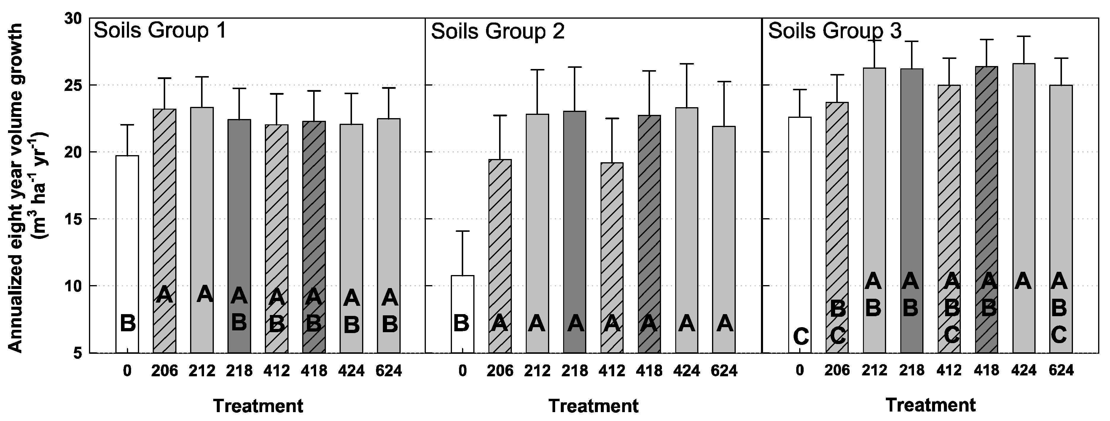
When including soil group in the treatment effects across site analysis, initial basal area (p ≤ 0.001), treatment (p ≤ 0.001), and treatment by soil group were significant. The average control volume growth eight years after treatment initiation was 19.7, 10.7 and 22.6 m³ ha⁻¹ yr⁻¹ for soil groups 1, 2 and 3, respectively (Figure 1). Average treated growth was 22.6, 21.8, and 25.6 m³ ha⁻¹ yr⁻¹ for soil groups 1, 2, and 3, respectively. Means separation tests indicated that the control treatment was significantly less than treatments 206 and 212, all treatments, and treatments 212, 218, 418, and 424 for soil groups 1, 2, and 3, respectively (Figure 1).

Figure 1. Eight-year average volume growth in soil groups 1, 2 and 3 for eight treatments where nitrogen was applied at different rates and frequencies across 22 sites in the southeastern United States. Different letters indicate significant differences in treatment means within a soil group. Error bars are one standard error.

Figure 1. Eight-year average volume growth in soil groups 1, 2 and 3 for eight treatments where nitrogen was applied at different rates and frequencies across 22 sites in the southeastern United States. Different letters indicate significant differences in treatment means within a soil group. Error bars are one standard error.

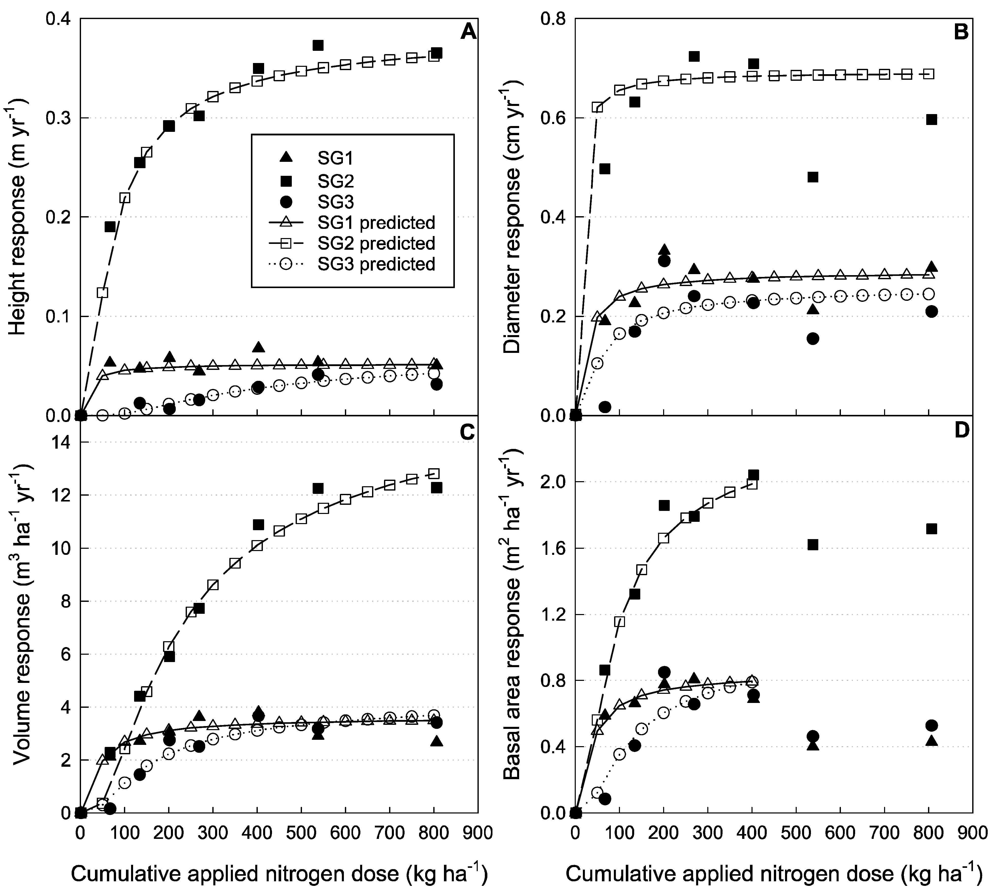
The asymptote (b₀) for all rate response functions was about the same for soil groups 1 and 3 (Table 7 and Figure 2A–D). The asymptote for soils group 2 was generally much greater than those for soil groups 1 and 3. For example, over the range of data, volume response for soil groups 1 and 3 reached an asymptote at about 3.5 m³ ha⁻¹ yr⁻¹ whereas soil group 2 sites achieved a volume response up to 12 m³ ha⁻¹ yr⁻¹ (Figure 2C). In contrast, the shape parameter (b₁) was significantly different for soil groups 1 and 3 for volume and basal area. The volume and basal area growth response increased much more rapidly in soil group 1 than in soil group 3 for applied nitrogen levels less than 300 kg ha⁻¹. For example, at a cumulative applied dose of 100 kg ha⁻¹ nitrogen, the estimated eight-year volume response reached 76% and 31% of the volume response predicted at 800 kg nitrogen ha⁻¹ for soil groups 1 and 3, respectively (Figure 2C). The shape parameter was not different for soil groups 2 and 3. There was little additional growth response for any of the growth variables for soil groups 1 and 3 sites after a cumulative dose of 300 kg ha⁻¹ of nitrogen had been applied. For soil group 2, the growth response continued to increase through the range of applied nitrogen (up to 800 kg ha⁻¹) for height and volume growth; however, the rate of increase in the growth response was reduced at higher nitrogen doses. The response models for basal area did not converge when including cumulative nitrogen doses greater than 400 kg ha⁻¹. Consequently, for the basal area response model presented here, data where the cumulative nitrogen dose was greater than 400 kg ha⁻¹ were excluded from the analysis.

Table 7. Parameter estimates, standard error, t values, lower and upper 95% confidence intervals (CI) for the height, diameter, volume and basal area growth response to increasing nitrogen dose functions. b₀ is the asymptote for soil group 3, b₀₁ and b₀₂ are adjustments to b₀ for soil groups 1 and 2, respectively. b₁ is the shape parameter for soil group 3, b₁₁ and b₁₂ are adjustments to b₁ for soil groups 1 and 2, respectively.

Parameter	Estimate	Standard error	Pr > t	Lower 95% CI	Upper 95% CI
Height
b0	0.066	0.042	0.120	−0.017	0.149
b01	−0.014	0.054	0.799	−0.120	0.092
b02	0.323	0.064	<0.001	0.197	0.450
b1	−350.1	174.0	0.045	−692.4	−8.521
b11	337.1	177.8	0.059	−12.25	686.4
b12	293.2	174.3	0.093	−49.30	635.7
Diameter
b0	0.259	0.041	<0.001	0.178	0.340
b01	0.032	0.060	0.602	−0.087	0.150
b02	0.434	0.071	<0.001	0.295	0.573
b1	−45.01	21.63	0.038	−87.54	−2.506
b11	25.75	28.01	0.358	−29.27	80.78
b12	39.58	22.58	0.080	−4.798	83.95
Volume
b0	4.350	1.066	<0.001	2.256	6.445
b01	−0.730	1.560	0.643	−3.788	2.343
b02	11.89	2.052	<0.001	7.862	15.92
b1	−134.1	24.97	<0.001	−183.1	−85.03
b11	103.6	29.70	<0.001	45.31	162.0
b12	−55.90	28.88	0.053	−112.7	0.815
Basal area
b0	1.033	0.196	<0.001	0.648	1.419
b01	−0.183	0.273	0.502	−0.721	0.354
b02	1.346	0.349	<0.001	0.661	2.032
b1	−107.1	25.74	<0.001	−157.7	−56.54
b11	80.04	31.06	0.010	18.97	141.1
b12	34.99	28.89	0.227	−21.80	91.78

Table 7. Parameter estimates, standard error, t values, lower and upper 95% confidence intervals (CI) for the height, diameter, volume and basal area growth response to increasing nitrogen dose functions. b₀ is the asymptote for soil group 3, b₀₁ and b₀₂ are adjustments to b₀ for soil groups 1 and 2, respectively. b₁ is the shape parameter for soil group 3, b₁₁ and b₁₂ are adjustments to b₁ for soil groups 1 and 2, respectively.

Parameter	Estimate	Standard error	Pr > t	Lower 95% CI	Upper 95% CI
Height
b0	0.066	0.042	0.120	−0.017	0.149
b01	−0.014	0.054	0.799	−0.120	0.092
b02	0.323	0.064	<0.001	0.197	0.450
b1	−350.1	174.0	0.045	−692.4	−8.521
b11	337.1	177.8	0.059	−12.25	686.4
b12	293.2	174.3	0.093	−49.30	635.7
Diameter
b0	0.259	0.041	<0.001	0.178	0.340
b01	0.032	0.060	0.602	−0.087	0.150
b02	0.434	0.071	<0.001	0.295	0.573
b1	−45.01	21.63	0.038	−87.54	−2.506
b11	25.75	28.01	0.358	−29.27	80.78
b12	39.58	22.58	0.080	−4.798	83.95
Volume
b0	4.350	1.066	<0.001	2.256	6.445
b01	−0.730	1.560	0.643	−3.788	2.343
b02	11.89	2.052	<0.001	7.862	15.92
b1	−134.1	24.97	<0.001	−183.1	−85.03
b11	103.6	29.70	<0.001	45.31	162.0
b12	−55.90	28.88	0.053	−112.7	0.815
Basal area
b0	1.033	0.196	<0.001	0.648	1.419
b01	−0.183	0.273	0.502	−0.721	0.354
b02	1.346	0.349	<0.001	0.661	2.032
b1	−107.1	25.74	<0.001	−157.7	−56.54
b11	80.04	31.06	0.010	18.97	141.1
b12	34.99	28.89	0.227	−21.80	91.78

Figure 2. Cumulative applied nitrogen rate response curves for height, diameter, volume and basal area (Panels A, B, C, and D, respectively) for three soil groups (SG1, SG2 and SG3) where nitrogen was applied at different rates and frequencies across 22 sites in the southeastern United States.

Figure 2. Cumulative applied nitrogen rate response curves for height, diameter, volume and basal area (Panels A, B, C, and D, respectively) for three soil groups (SG1, SG2 and SG3) where nitrogen was applied at different rates and frequencies across 22 sites in the southeastern United States.

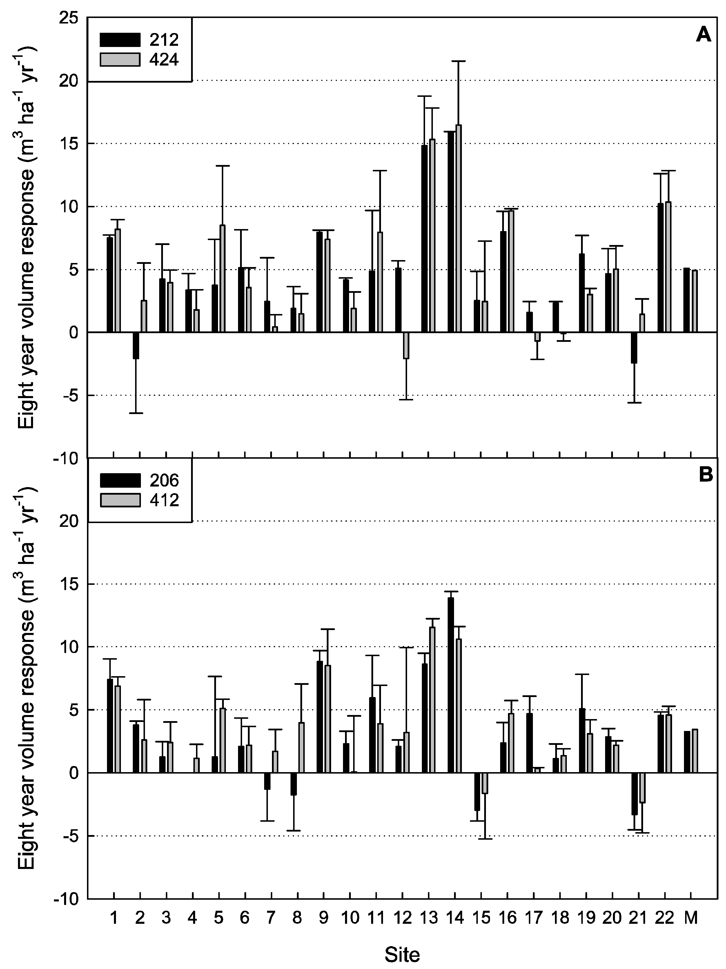
There were no significant differences observed in the frequency of application comparisons as long as the total applied dose was the same. The response from treatment 212, where 134 kg ha⁻¹ nitrogen was applied every two years (average of 5.1 m³ ha⁻¹ yr⁻¹ for eight years), was no different than the response from treatment 424, where 268 kg ha⁻¹ nitrogen was applied every four years (p = 0.687) (average of 4.9 m³ ha⁻¹ yr⁻¹ for eight years) (Figure 3A). A similar result was observed in the comparison between treatments 206 and 412 (p = 0.555). The average responses from treatment 206, where 67 kg ha⁻¹ nitrogen was applied every two years, and treatment 412, where 134 kg ha⁻¹ nitrogen was applied every four years, were 3.1 and 3.4 m³ ha⁻¹ yr⁻¹ for eight years, respectively (Figure 3B).

Figure 3. Comparison of treatments where the same cumulative nitrogen dose was applied at different rates and frequency of application across 22 sites in the southeastern United States and the mean (M) across all sites. Panel A shows the comparison where 538 kg ha⁻¹ of nitrogen was applied as four applications of 134 kg ha⁻¹ every two years or as two applications of 269 kg ha⁻¹ every four years. Panel B shows the comparison where 269 kg ha⁻¹ of nitrogen was applied as four applications of 67 kg ha⁻¹ every two years or as two applications of 134 kg ha⁻¹ every four years. Error bars are one standard error.

Figure 3. Comparison of treatments where the same cumulative nitrogen dose was applied at different rates and frequency of application across 22 sites in the southeastern United States and the mean (M) across all sites. Panel A shows the comparison where 538 kg ha⁻¹ of nitrogen was applied as four applications of 134 kg ha⁻¹ every two years or as two applications of 269 kg ha⁻¹ every four years. Panel B shows the comparison where 269 kg ha⁻¹ of nitrogen was applied as four applications of 67 kg ha⁻¹ every two years or as two applications of 134 kg ha⁻¹ every four years. Error bars are one standard error.

4. Discussion

We accepted our first hypothesis because site was a significant factor in the analyses examining treatment effects for individual sites, where eight sites had a significant treatment effect (Table 5), and in the across site analysis where site was a significant factor. Soil group was also a significant factor in the across site analysis. Grouping sites on soils is a useful tool for managers interested in determining which stands are the best candidates for adding resources [24]. Most of the studies had two replications, which reduces the ability to detect differences due to treatment at individual sites. However, use of the two-replication studies allowed more installations across the landscape, which improved our ability to examine the second and third hypotheses at the regional scale. Regardless, the growth responses at the soil group 2 sites were large, such that all of the soil group 2 sites had significant responses to treatment when examined as individual studies, and the soil group 2 sites had a larger response to treatment than the other soil groups (Figure 2). From a management perspective, while the response to fertilization was dramatic at the soil group 2 sites, these sites required more applied nutrients to achieve the same level of absolute growth than the sites in soil groups 1 and 3 (Figure 1 and Figure 2C). This study provides information managers can use to determine which stands will likely respond to treatment from a biological perspective while having an understanding of what it will take to achieve that biological potential from an economic perspective.

We accepted our second hypothesis that the volume growth rate response curve was not linear (Figure 2). Volume growth response reached an asymptote for soil groups 1 and 3 at a cumulative dose between 300–400 kg ha⁻¹ of applied nitrogen. The response curve for soil group 2 continued to increase through the maximum cumulative applied nitrogen dose of 800 kg ha⁻¹. The rate of growth increase was greater for soil group 1 than for soil group 3 (significant shape parameter b₁₁ in Table 7). Soil group 1 sites are poorly drained and may have been able to capitalize on available water to take up the newly available nutrients more readily than those in soil group 3, which were located on well-drained sites. The two-year response data used to develop the response function may underestimate the true response because the trees only had a short time to respond, although this effect would likely be experienced across all sites. However, without the two-year response data, the rate response analysis would have no low doses and the model becomes insensitive to changes in the b₁ coefficient.

The observed growth responses from soil groups 1 and 3 were in the same range as previous reports where response to nitrogen was linear through 336 kg ha⁻¹ of applied nitrogen [10,19]. The large response observed from soil group 2 was in the same range as the data from the literature for an equivalent amount of nitrogen. In our study, the application of 224 kg ha⁻¹ nitrogen resulted in a response of 7 m³ ha⁻¹ yr⁻¹ for eight years, and Rojas [19] found studies with responses of approximately 7.5 m³ ha⁻¹ yr⁻¹ over eight years from an equivalent nitrogen application. The response at the soil group 2 sites was impressive; however, the control plots at these site were growing relatively slowly at 10.7 m³ ha⁻¹ yr⁻¹. Average treated growth was (22.6, 21.8 and 25.6 m³ ha⁻¹ yr⁻¹ for soil groups 1, 2, and 3, respectively) lower than modeled potential productivity of loblolly pine in the southeast United States (>30 m³ ha⁻¹ yr⁻¹) [5] and that observed in individual studies where treatments were applied with the intent to eliminate all resource limitations (up to 35 m³ ha⁻¹ yr⁻¹) (e.g., [8,29,30]). Clearly, the sites in our study were nitrogen and phosphorus limited. After these limitations were ameliorated with our treatments, other resource limitations such as water, other nutrients, light and space would influence productivity, following Liebig’s Law of the Minimum.

We accepted our third hypothesis that the overall applied nitrogen dose and not application frequency determined the growth response. None of our treatments were single dose applications, however, our data are in agreement with a study where the same dose of nitrogen was applied in either one or two applications two years apart, with both treatments providing similar responses in southern pine [31]. As mentioned previously, our responses were in the same range as other studies where applications up to 336 kg nitrogen ha⁻¹ were applied in single doses [10,19]. Our results are consistent with those found in Eucalyptus grandis where a similar range of doses (60 to 240 kg ha⁻¹ of applied nitrogen) was applied at 1, 2, 3, and 6 application frequencies to achieve the same cumulative dose, and only one of eleven tests indicated a difference in growth response at the end of the study period (3 years in this case) [32]. Reductions in fertilizer applications on a regional scale are likely a result of high material prices [33]. At the same time, urea prices (the most common form of nitrogen used in forestry application) can fluctuate by large amounts in relatively short periods of time [34]. Consequently, this result provides managers more flexibility in planning for nutrient additions.

The age at study initiation ranged from two to six years old. For stands at the low end of this range, the assart effect may still have been providing nutrients, and yet these young stands were responsive to additional nutrients applied in this study. The assart effect is generally applicable to nitrogen availability. However, sites that would likely be phosphorus limited (poorly drained coastal plain sites) received phosphorus at planting and competing vegetation was relatively low at study initiation. Consequently, the rapid early response in our studies was likely from amelioration of nitrogen limitations. Even if resources continued to be available from the assart effect, the magnitude of resource availability from this effect would be relatively small compared with the application rates in this study. As noted in previous studies, loblolly pine is a very plastic species and responds well to large amounts of nutrient inputs [8,9,30,35]. This rapid growth early in the rotation (typical rotation length of 20–25 years) resulted in a situation where some stands reached stocking levels that would indicate the need for a thin. Based on Reineke’s [36] maximum stand density index of 450 for loblolly, and Drew and Flewelling’s [37] estimate that density dependent mortality begins at 50%–55% of maximum stand density index, sites with basal areas greater than approximately 23 m² ha⁻¹ would begin to have intraspecific competition. All of the 424 treatment stands had basal areas greater than this amount and some sites (3, 10, and 21) had basal areas greater than 40 m² ha⁻¹ eight years after treatment initiation. If juvenile fertilization is included in a silvicultural prescription, then it is likely that thinning may need to be considered earlier than what might be considered normal. Density-dependent mortality may have resulted in the failure of the basal area rate response model to converge for cumulative nitrogen doses greater than 400 kg ha⁻¹ of nitrogen. In these cases, mortality may have reduced basal area responses below what would be expected if over-stocking had not occurred.

5. Conclusions

Juvenile southern pine stands will respond to fertilizer. Sites in this study were limited by nitrogen and phosphorus and they responded to nutrient applications at young ages. Soil texture and drainage were useful in categorizing the sites for potential response. Soils with clay subsoil reached an asymptotic response between 300 and 400 kg ha⁻¹ of applied nitrogen. Cumulative nitrogen dose, and not application frequency or dose, determined the response. When undertaking juvenile fertilization, the silvicultural prescription should include consideration for rapid stand development.