Article

Towards Automated Characterization of Canopy Layering in Mixed Temperate Forests Using Airborne Laser Scanning

1
Remote Sensing Laboratories, University of Zurich, Winterthurerstrasse 190, Zurich CH-8057, Switzerland
2
Institute of Mathematics, University of Zurich, Winterthurerstrasse 190, Zurich CH-8057, Switzerland
*
Author to whom correspondence should be addressed.
Forests 2015, 6(11), 4146-4167; https://doi.org/10.3390/f6114146
Submission received: 18 September 2015 / Revised: 10 November 2015 / Accepted: 12 November 2015 / Published: 18 November 2015

Abstract

:
Canopy layers form essential structural components, affecting stand productivity and wildlife habitats. Airborne laser scanning (ALS) provides horizontal and vertical information on canopy structure simultaneously. Existing approaches to assess canopy layering often require prior information about stand characteristics or rely on pre-defined height thresholds. We developed a multi-scale method using ALS data with point densities >10 pts/m2 to determine the number and vertical extent of canopy layers (canopylayer, canopylength), seasonal variations in the topmost canopy layer (canopytype), as well as small-scale heterogeneities in the canopy (canopyheterogeneity). We first tested and developed the method on a small forest patch (800 ha) and afterwards tested transferability and robustness of the method on a larger patch (180,000 ha). We validated the approach using an extensive set of ground data, achieving overall accuracies >77% for canopytype and canopyheterogeneity, and >62% for canopylayer and canopylength. We conclude that our method provides a robust characterization of canopy layering supporting automated canopy structure monitoring.

1. Introduction

Forests provide a wide range of valuable ecosystem goods and services [1]. Understanding forest ecosystems and their underlying processes help with forecasts using scenarios under global change conditions and supports the establishment of sustainable management strategies [2,3,4,5]. The three-dimensional distribution of geometric objects and their topology within a forest canopy (termed “canopy structure” [6,7] is considered a particularly crucial constituent of forest ecosystems’ functioning and processes. Canopy structure can, among other things, serve as an indicator of forest stand resistance to disturbances [8,9], enable the estimation of the conservation potential for biodiversity [10,11], or allow the identification of recruitment limitations [12,13]. Canopy structure itself is not a measurable quantity, but the properties of canopy structure can be described by means of a wide variety of structural variables, such as tree height, tree diameter distribution, or canopy layering [14]. The assessment of canopy layering, in particular, is of great importance. Canopy layers provide essential structural components of wildlife habitat [15], affect stand productivity [16], and are used to manage forest stands and to identify forest structural stages [17]. From the various existing definitions of canopy layer (cf. [18]), we follow Franklin and Spies [19] and understand canopy layer as continuous vertical distribution of foliage within the canopy.
Traditionally, canopy layering is assessed by conventional fieldwork in relatively small areas, which is time-consuming and occasionally subjective [20,21]. Advances in Earth observation systems and analysis techniques have greatly improved the ability to characterize canopy structure over large areas in not only the horizontal but also the vertical dimension [22,23,24]. In particular, light detection and ranging (LiDAR) systems, especially airborne laser scanning (ALS), are suitable to provide very detailed vertical and horizontal information on canopy structure based on the physical measurement principle of active sensing and full-waveform digitization [25,26,27,28]. This also means that definitions of canopy layering which, for example, focus more on composition of life forms or age classes cannot be taken into consideration, as the types of physical measurement possible with ALS do not meet these definitions.
ALS-based assessment of canopy layering can be either derived from LiDAR waveform data (mostly the case for large or medium-footprint LiDAR systems) [29,30,31], or based on ALS point clouds directly [32,33] or indirectly, e.g., by generating a kind of synthetic waveform using classified echo height distributions or height distribution probability functions [34,35,36]. The assessment of canopy layering with ALS is mainly performed using area-based approaches (ABA). The spatial scale of ABA is currently often driven by user requirements and usually limited by the features present in the available data [37]. However, the choice of a specific spatial scale affects the canopy layer analysis, as a decrease in horizontal resolution will result in more mixing of horizontal and vertical structure elements within each spatial unit [34,35,38,39]. Most canopy-structure components, however, have inherent spatial scales and the choice of the spatial scale should be made considering the investigated structural component [40,41]. Nevertheless, an acceptable compromise often needs to be found between the technical capabilities of ALS and user needs, such as the application domain or cost-benefit considerations [42,43]. In this study, ABAs represented in regularly spaced grids were used, allowing flexible analysis in terms of spatial scales and cross-scale comparisons (e.g., testing reproducible up- and down-scaling methods).
ABA’s were investigated by Wulder et al. [25,44], White et al. [45], and Næsset [46] who found the concept to be sufficiently robust for operational use. The assessment of canopy layering, however, is rarely considered. Existing approaches to assess canopy layers often require a substantial set of prior information about stand characteristics or rely on pre-defined height thresholds for an existing stratification of the canopy. Whitehurst et al. [30], for example, on one hand used the cumulative canopy cover and pre-defined height thresholds to distinguish between understory (0 to 5 m), midstory (5 to 15 m), and overstory (>15 m). On the other hand, the peaks of the LiDAR waveform were used to determine canopy layers, assuming that each peak represents the mean layer height. The peak definition parameters, however, were determined by visual analysis [30]. Ferraz et al. [32] applied a mean shift segmentation algorithm to determine the modes of the distribution functions of echo heights and afterwards defined thresholds to divide the canopy into overstory, understory and ground vegetation. In this context, the definition of these thresholds remains critical as one component of the algorithm is linked to a function of canopy layer depth and thus depends on the tree species and/or forest biome [32]. Wang et al. [35] also used the modes of echo height distribution functions to divide the canopy into single-layered and double-layered canopies. Furthermore, the length of the determined layers was estimated, whereby only changes in absolute point density (i.e., inflexion points in the height distribution function) were used as the criterion to define the borders of a layer, which are not necessarily coincident. Maltamo et al. [36] also distribution functions of echo heights, in a manner comparable to Whitehurst et al. [30], Ferraz et al. [32], and Wang et al. [35], to relate the modes of the function (i.e., unimodal or multimodal) to the amount of canopy layers. In contrast, however, a fundamental part of their algorithm was the prior definition of a threshold to separate the dominant tree layer and understory trees, which limits the determination of canopy layers to a maximum of two layers. Morsdorf et al. [33] applied a cluster analysis to echo heights and echo intensities to stratify the canopy into three layers, whereby each layer consists almost entirely of oak, pine or shrubs, respectively. Although the proposed approach results in high accuracy values, a successful transfer of the method to dense, mixed temperate forests is unlikely. Zimble et al. [43] used a LiDAR-based canopy height model for the identification of individual trees and to determine their respective heights. The variances in tree heights were subsequently analysed on a 30 × 30 m cell size and used to distinguish between single-layered and multi-layered canopies. Accordingly, only trees forming the top canopy layer were considered and the resulting canopy stratification is more related to the composition of age classes and less to the actual vertical foliage distribution. Possible canopy layers below the top canopy layer, however, could not be assessed.
Therefore, most of the existing approaches are limited in their transferability to other sites and they tend not to be directly comparable. The inherent spatial scales of canopy-structure components are barely considered and, to our knowledge, a multi-scale approach regarding canopy layering has so far only been presented by Wang et al. [35]. To overcome these limitations, we propose using an automated and transferable ABA to provide quantitative assessments of canopy layering at different scales.

Aim and Research Objectives

The aim of this study is to develop a transferable, grid-based assessment of canopy layering. Requirements are defined using a stakeholder approach, originating from the forestry department of the Canton of Aargau, Switzerland, a regional authority responsible for forest management. The requirements were to assess canopy layering, canopy length, canopy type and small-scale heterogeneity of the canopy using an automatic and transferable approach with a target grid-cell size of 10 m × 10 m). Accordingly, the main objectives of this study were (i) to determine and classify the number and vertical extent of canopy layers; (ii) to distinguish between deciduous and evergreen forest stands; (iii) to characterize the small-scale heterogeneity of the canopy; and iv) to test the robustness and transferability of the method to a significant portion of forested land within the Canton of Aargau. The derived canopy-structure descriptors (canopylayer, canopylength, canopytype and canopyheterogeneity) as well as their spatial distribution were validated using an extensive set of field data.

2. Study Area and Data
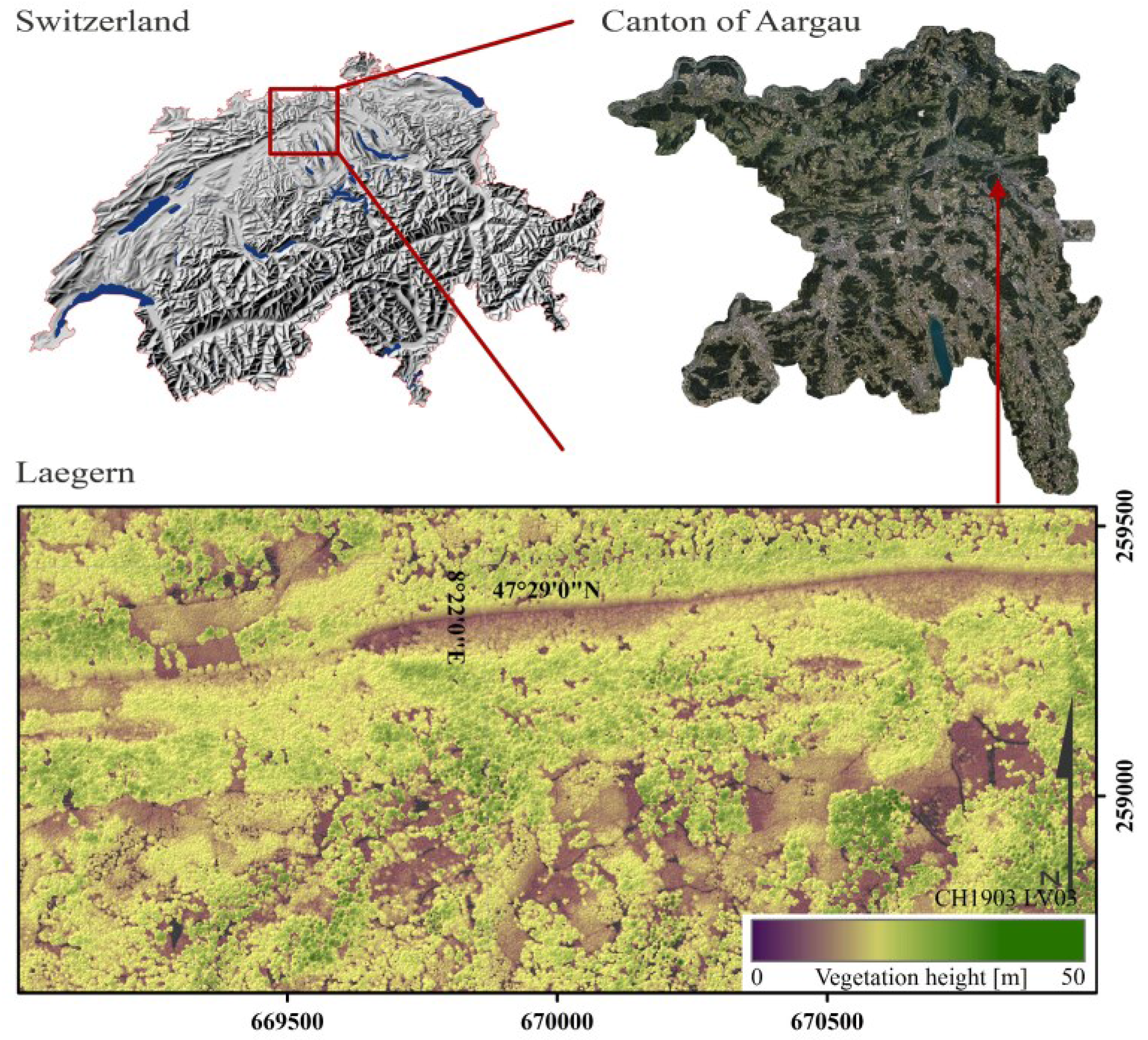
2.1. Study Site

We developed and tested the method at the Laegern site (47°28′ N, 8°21′ E), a temperate forest located in Canton of Aargau, Switzerland (Figure 1). The site is approximately 800 ha and mainly composed of mixed deciduous forest, dominated by common beech (Fagus sylvatica L.), European ash (Fraxinus excelsior L.), and sycamore maple (Acer pseudoplatanus L.), with scattered silver fir (Abies alba Mill.) and Norway spruce (Picea abies L.) trees [47,48].
Figure 1. Switzerland (left) and the location of Canton of Aargau (right, top panel). Laegern experimental site (800 ha forested area) plotted against ALS-derived canopy height (bottom panel).
Forests 06 04146 g001
To prove the transferability and robustness of the approach, the method was subsequently transferred to the entire area of Canton of Aargau (180,000 ha) without adapting the algorithm, including areas undergoing different forest management practices (ranging from natural forests to highly intensive regimes with silvicultural interventions) and a variety of forest types.

2.2. Reference Data

An extensive set of ground based reference measurements was collected for the Laegern site between 2012 and 2014. We applied a stratified sampling, where strata correspond to development stages (age classes) and canopy type (evergreen/deciduous), resulting in 200 sample plots with an approximate size of 100 m2 per plot. Plot-wise measurements were taken for forest structure information on the individual tree level, such as tree position, social position, crown dimensions, tree vitality, tree height, tree species, and diameter at breast height for all trees with a diameter at breast height (DBH) larger than 20 cm (cf. [34]). The tree positions were precisely measured based on terrestrial land surveying using a total station and a differential GPS system, linked to fixed points of the Swiss national survey. Tree species were afterwards aggregated into the canopy type’s “deciduous canopy” and “evergreen canopy”.
Forest experts interpreted for an area within 10 m around each tree position’s canopy layering and estimated the canopy length based on hypsometer measurements. In this regard, it must be noted that for canopies with two or more layers, it is assumed that measurements of the canopy length become increasingly uncertain. The small-scale heterogeneity was visually assessed in consideration of variations in DBH, crown base and the canopy length. Even if foresters’ interpretation of canopy structure is often subjective and depends on the applied definitions (cf. [18]), it is the only non-destructive solution so far known to us to assess these types of canopy-structure descriptors. The information about canopy layering, canopy length, canopy type, and small-scale heterogeneity was transferred to a grid-based representation with a 10 m × 10 m grid-cell size.
For the entire forested area of Canton of Aargau, stand maps were available as polygon layers [49]. The stand maps were produced by regional foresters, containing detailed descriptions of canopy type, canopy layering and canopy length as well as current forest management practices. To ensure the spatial and temporal comparability of the stand maps with the ALS-derived canopy structure information, we used only stand polygons updated in the years 2012–2014. Reference data thusly derived contain more than 16,000 stand polygons, distributed over the entire area of Canton of Aargau.

2.3. Airborne Laser Scanning Data

In the approach presented in this study, we used full-waveform ALS data. The ALS data for the Laegern site were acquired in 2010 under both defoliated (or leaf-off) and foliated (or leaf-on) conditions. The ALS data for Canton of Aargau were acquired in 2014. The used sensor specifications are summarized in Table 1 and described more in detail in [50,51].
Table 1. Used sensor specifications of RIEGL’s airborne laser scanner LMS-Q560 and LMS-Q680i (RIEGL Laser Measurements Systems GmbH, Austria) for the Laegern site and Canton of Aargau.
Laegern (2010)Canton of Aargau (2014)
ALS SensorLMS-Q560LMS-Q680iLMS-Q680i
Mean operating altitude above ground (m)500600700
Scanning methodrotating multi-facet mirror
Pulse detection methodfull-waveform processing
Pulse length (nanoseconds)<4
Sampling interval (nanoseconds)1
Scan angle (degree)±15±22
Mean point density (pts/m2)20401530
Date of acquisition10 April01 AugustMarch/AprilJune/July
The benefit of full-waveform data is the approximation of the entire backscattered signal by digitization, which facilitates the extraction of additional features of each reflecting object within the ALS footprint. To detect and extract specific object reflections, Gaussian pulse estimation was applied using Riegl’s software RiANALYZE 3.0.8 (RIEGL, Horn, Austria) [52] in order to obtain representative echo descriptions (cf. Figure 2). This includes the derivation of a three-dimensional point cloud composed of planimetric coordinates (x and y), ellipsoidal heights (z) and echo type (i.e., first, intermediate, last echo). Additionally, it enables the physical description of each reflector with information such as amplitude, width and intensity of each specific echo.
Figure 2. Physical concept of airborne laser scanning: interaction of the emitted laser pulse with the vegetation canopy (left panel), the full and the decomposed waveform (middle panel), and the resulting echo descriptors.
Forests 06 04146 g002
For the ALS data of the Laegern site, the terrain-corrected point cloud was derived by extracting potential ground returns from the point cloud while retaining single and last echoes, together with their geometrical characteristics and the corresponding echo-width information. Detection and filtering of the ground returns was carried out using an adaptive multi-scale filter [53]. A 0.5 m × 0.5 m digital terrain model (DTM) was generated from the remaining points using an ordinary kriging interpolation. For the ALS data of Canton of Aargau, a DTM with a spatial resolution of 0.5 m × 0.5 m was processed by MILAN Geoservice GmbH using the Terrasolid software (Terrasoild, Helsinki, Finland). For both data sets, the height above ground was then calculated for each echo of the point cloud by subtracting the interpolated DTM value at the corresponding horizontal echo location. For the subsequent use of the point clouds, we used only the planimetric coordinates and terrain-corrected heights.

3. Methods

3.1. Stakeholder’s Requirements

The thematic framework for our research was established by stakeholder requirements. According to these requirements, we defined canopy-structure descriptors and appropriate descriptor classes (Table 2).
Table 2. Stakeholder’s requirements for a grid-based assessment of canopy layering and according canopy-structure descriptors used in this study.
Canopy-Structure Descriptors (Acronym)Definition According Stakeholder’s Requirements
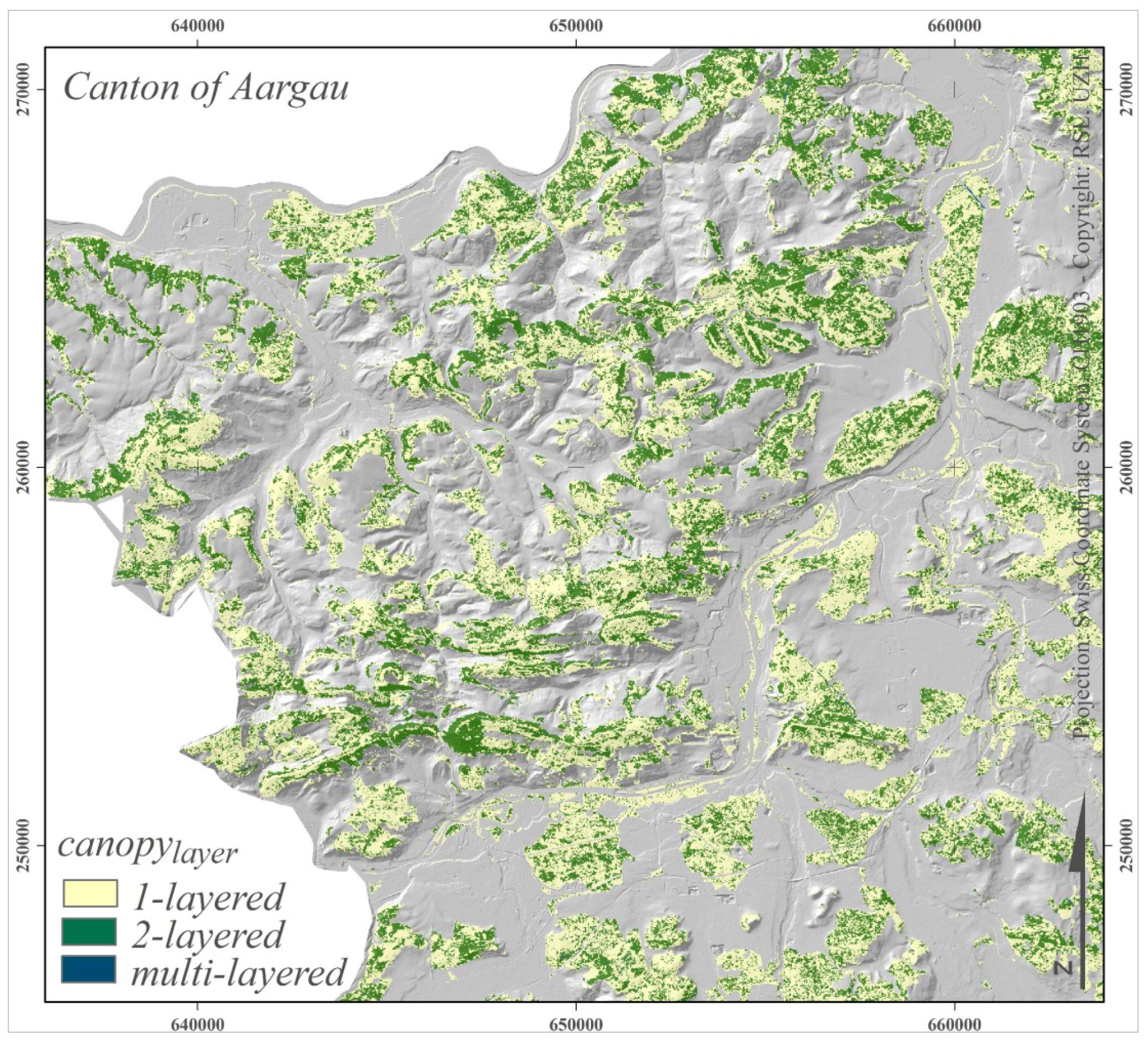
Canopy layering (canopylayer)A canopy layer consists of a continuous, vertical foliage distribution. A canopy layer must be ≥3 m in vertical extent. Gaps in the canopy must be ≥3 m in vertical extent to result in a separation/ delimitation of canopy layers. Three classes should be distinguished:
  1. 1-layered canopy
  2. 2-layered canopy
  3. multi-layered canopy (>2 canopy layers)
Canopy length (canopylength)Classified ratio of the length of the topmost canopy layer (vertical extent in m) and the total canopy height. Two classes should be distinguished:
    1. short/medium canopy (ratio of <0.5)
    2. long canopy (ratio of ≥0.5)
Canopy type (canopytype)Distinction between canopies, shedding or losing foliage at the end of the growing season, and canopies having leaves throughout the year. Two classes should be distinguished:
    1. deciduous canopy
    2. evergreen canopy
Small-scale heterogeneity (canopyheterogeneity)Small-scale variation of vertical foliage distribution within each 10 m × 10 m grid cell. Significance of variation should be defined using the p-value with a significance level of 0.05. Two classes should be distinguished:
    1. homogeneous canopy (non-significant variation)
    2. heterogeneous canopy (significant variation)

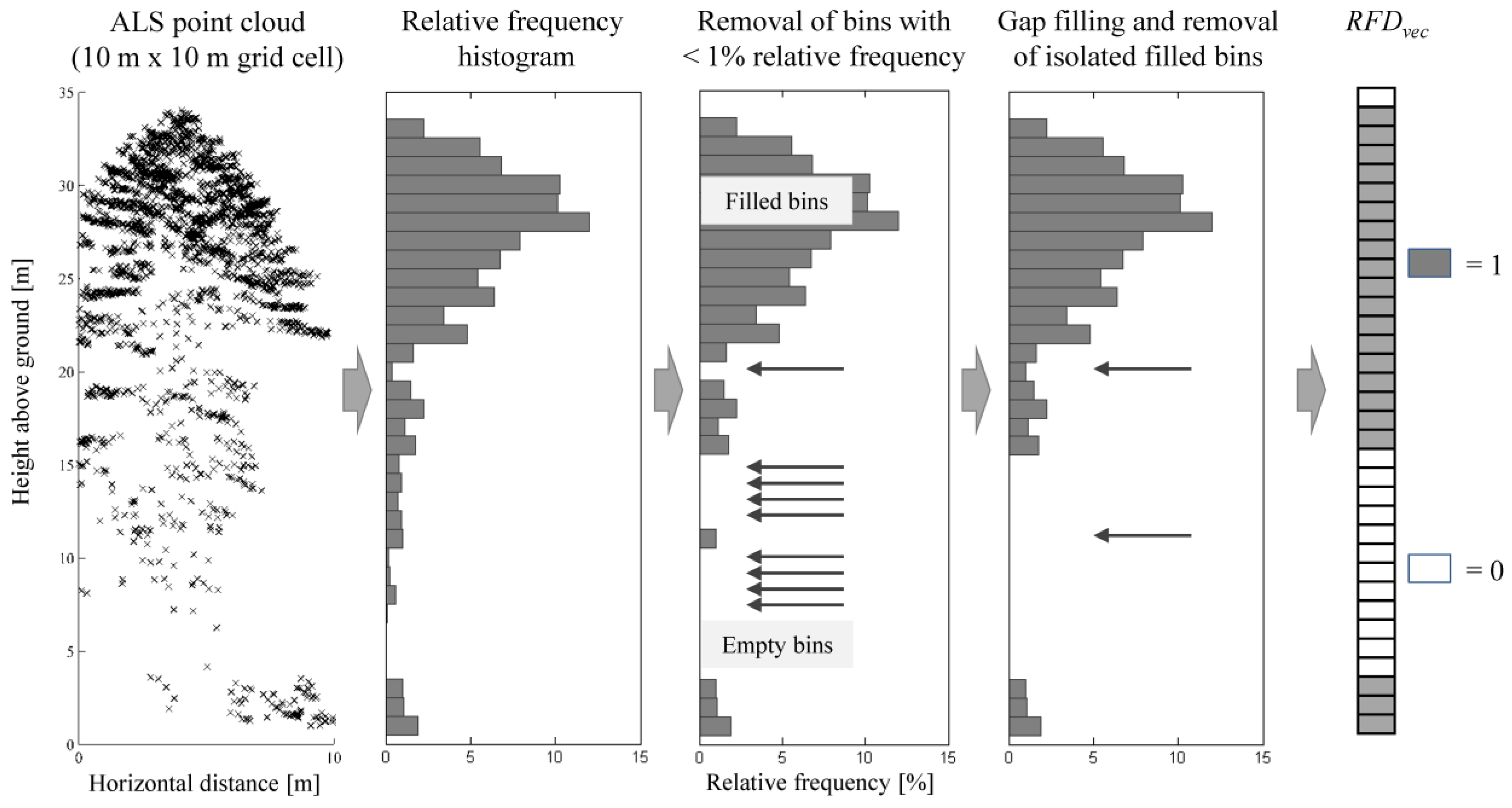
3.2. Calculation of the Relative Frequency Distribution

One of the essential feature of our method is the relative-frequency distribution (RFD) of echo heights within a given grid cell. This means that all echo returns within a grid-cell were binned according to height above ground [54], whereby the bin size was set to 1 m. Thus, the RFD shows the echo occurrences (echobin) for all height intervals/bins (γ) up to the maximum echo height (γN) as a percentage of the total number of echoes (echototal) (Equation (1)).
R F D ( γ )   =   e c h o b i n ( γ ) e c h o t o t a l                             , γ [ y 0 , y 1 , y N ]
Those RFDs can be displayed as relative-frequency histograms (often called pseudo-waveforms in the literature) and should comprehensively represent the ALS-based characterization of the vertical canopy structure, although this is not necessarily a complete representation of the actual canopy structure (cf. [39,55]). Nevertheless, previous studies emphasized and proved the potential of RFDs for comprehensive canopy-structure characterization [35,54,56,57].
For our study, the definition of a grid-cell size of 10 m × 10 m to derive RFDs was according to the dimensions of the reference data and the user requirements, which is a common practice (cf. [25,45]). In a previous study [34], however, we determined based on a data-driven approach that the best feasible grid-cell size was 8 m × 8 m for canopy-structure characterization. Muss et al. [54] also concluded that a grid-cell size between 10 and 15 m was optimal to assess forest-canopy structure using RFDs. Therefore, the applied user-defined grid-cell size in our case was in line with “optimal” grid-cell sizes determined in recent research findings.
To assess the small-scale heterogeneity, we defined a small-scale grid-cell size of 1 m × 1 m and derived RFDs in the same way as described before. The definition of the fine-scale grid-cell size was deduced from the positional accuracy of the point cloud, the point density and the footprint diameter of the laser pulse (cf. [58]). As we showed in a previous study [34], the point density was not a limiting factor: Even for the small grid-cell size of 1 m × 1 m, the available point cloud has almost the maximum achievable information on the canopy structure that current ALS systems can provide. This means that a further increase in point density would not significantly change the derived RFDs.
Following Lefsky et al. [31], a threshold value of 1% was used to classify each RFD bin into either “filled” (relative frequency ≥ 1%) or “empty” (relative frequency < 1%). Filling single, isolated empty bins smoothed the derived RFD. Isolated empty bins can be either caused by smaller gaps in the canopy (below the stakeholder’s definition of 3 m in vertical extent, cf. Table 2) or by occlusion effects and are thus not considered large enough to separate independent canopy layers. The same approach was used to remove isolated filled bins (below the stakeholder’s definition of 3 m in vertical extent, cf. Table 2). Finally, the RFD was converted to a vector RFDvec with “1” for filled bins and “0” for empty bins. Figure 3 shows the processing from the terrain corrected ALS point cloud to the filtered RFDs, which were used for the subsequent calculation of canopy-structure descriptors.
Figure 3. Processing steps from the ALS point cloud to the filtered RFDvec for a selected 10 m × 10 grid-cell.
Forests 06 04146 g003

3.3. Calculation of Canopy-Structure Descriptors

For the assessment of canopy layering (canopylayer), we first investigated the added value of the multi-seasonal ALS data. Kükenbrink et al. [59] investigated occlusion effects based on a 1 m voxel grid, showing that particularly for ALS acquisition under leaf-on conditions, large parts of the canopy volume were occluded. Therefore, we derived the RFDs of the leaf-on/leaf-off ALS data separately and correlated them to the RFD based on the combined point cloud (cf. [34]). It turned out that RFDs based on the leaf-on data show a high correlation of >95% to their respective histogram based on the combined point cloud, whereas the leaf-off derived RFDs mainly contain redundant information about the canopy layering (cf. [34]). This may indicate that the occluded volume in the leaf-on acquisition is often “empty” space without structural components. Thus, the underestimation of foliage and foliage distribution would be less significant than expected. Moreover, in particular for deciduous canopies, the leaf-off RFDs more likely represent stems and branches instead of actual foliage, which does not meet the definitions of canopy layering we used. We thus decided to use the leaf-on RFDs only to assess canopy layering, canopy length and the small-scale heterogeneity of the canopy.
Starting from the topmost filled bin, we applied a convolution kernel K to RFDvec, which determines vector positions with changes from “0” to “1” and vice versa (cf. Equation (2)). According to K, changes from “0” to “1” result in “1” and indicate the start of a layer, whereas changes from “1” to “0” result in “−1” and indicate the end of a layer. Accordingly, the sum of positive changes (“1”) is related to the amount of canopy layers (canopynumber).
c a n o p y n u m b e r =   K * R F D v e c > 0 0 ,    K = [ ˗ 1 , 1 ]
According to the requirements defined in Table 2, we classified canopynumber into canopylayer with the classes “1-layered”, “2-layered” and “multi-layered” canopy. The length of the topmost canopy layer was subsequently determined in RFDvec by the sum of filled bins, starting from the topmost filled bin to the first change from “1” to “0”. Following, we calculated the canopy ratio as the length of the topmost canopy layer divided by the total canopy height. To obtain canopylength, the canopy ratio was classified into “short canopies” (canopy ratio < 0.5) and “long canopies” (canopy ratio ≥ 0.5).
Using both the RFDs based on leaf-off and leaf-on data, we calculated the differences in relative frequencies in the topmost canopy layer as proxy for canopytype. We classified the difference values into significant differences and non-significant differences using the p-value with a significance level set to 0.05. To test the statistical hypothesis, we applied a Welch’s test [60]. Significant differences, which are mainly caused by changes in the leaf volume, indicate a “deciduous canopy”, whereas non-significant differences indicate an “evergreen canopy”.
The small-scale heterogeneity of the canopy (canopyheterogeneity) was derived using the RFDs derived on 1 m × 1 m (RFDsmall) and the corresponding RFD derived on 10 m × 10 m (RFDlarge). Each RFDsmall was compared to the specific RFDlarge using the empirical correlation coefficient rxy (e.g., [61]). The average rxy for the respective 10 m × 10 m grid cell was afterwards used to describe canopyheterogeneity. Comparable to the applied classification of canopytype, the classification into homogenous canopy (“non-significant variation”) and heterogeneous canopy (“significant variation”) was carried out based on the p-value with a significance level set to 0.05. The statistical hypothesis was tested using the t-test [60]. “Significant variations” reveal a high variability in RFDsmall within a 10 m × 10 m grid cell and thus point to a worse representation of the actual vertical structure by RFDlarge in contrast to a low variability of RFDsmall, indicated by “non-significant variations”.
The resulting canopy-structure descriptors canopylayer, canopylength, canopytype, and canopyheterogeneity were validated on the Laegern site with the forest inventory data for the canopy-structure descriptors based on both the 2010 and on the 2014 data. For the entire Canton of Aargau, we validated canopylayer, canopylength, and canopytype only, as until now canopyheterogeneity has not been a used/defined variable for canopy-structure characterization at the stand level. For the applied accuracy assessment, we calculated the widely used error matrix metrics “overall accuracy”, “user’s accuracy”, “producer’s accuracy”, and the “Kappa coefficient” [62]. Overall accuracies are computed by dividing the total correct classified grid cells by the total number of grid cells for each canopy-structure descriptor. Producer’s accuracies indicate the probability of a “reference grid cell” being correctly classified and user’s accuracies indicate the probability that the classified canopy-structure descriptor represents the “reference grid-cell”. According to Rosenfield & Fitspatrick-Lins [63], the Kappa coefficient is the proportion of agreement after chance agreement is removed.
To estimate the comparability of the field measurements done for the Laegern site with the information contained in the stand polygons, we validated the canopy descriptors based on the 2010 and the 2014 data independently and each with both sources of reference data.

4. Results

For the Laegern site, the validation shows promising results for all canopy-structure descriptors. The validation results for the canopy-structure descriptors are listed in Table 3, including the differentiation between the ALS and reference data used. The different ALS and reference data used influence the accuracy values of the derived canopy-structure descriptors only to a small degree. Nevertheless, all canopy-structure descriptors derived from the ALS data of 2010 show higher accuracies except for canopytype. On average, the validation with the forest inventory data of the Laegern site results in slightly higher accuracies in comparison to the validation results based on the stand polygons of the Canton of Aargau. With 2.4% (cf. Table 3), however, the mean difference in overall accuracies caused by the used reference can be more or less neglected. The same applies for differences in the overall accuracies caused by the different ALS data used with a mean difference of 3.1%. Particularly in terms of the determination of canopytype and canopyheterogeneity, the developed algorithm shows a good performance. The classification of canopytype leads to high overall accuracies up to 89.5%. The highest overall accuracy for canopyheterogeneity is reached with 81.5%. Overall accuracies up to 66.0% are achieved for canopylength, whereby misclassifications mainly occur in 2- or multi-layered forest stands. Canopy layering (canopylayer) is derived with an overall accuracy of 67%, ranging from 80% (1-layered canopies) to 53.3% (multi-layered canopies). The highest overlap occurs between the 2- and multi-layered canopy classes. In general, most classification uncertainties are caused by continuous transition zones between forest stands differing in age and structure. For these regions an accurate separation (e.g., in terms of a definition of a borderline between a 1-layered and a 2-layered canopy) is complex, even more so in the field.
Table 3. Accuracy assessment of the canopy-structure descriptors for the Laegern site. We use the accuracy metrics “overall accuracy” (OA), “user’s accuracy” (UA), “producer’s accuracy” (PA), and the “Kappa coefficient” (K). Resulting values in italics represent results obtained from stand polygons.
Canopy-Structure DescriptorsALS Data (2010)ALS Data (2014)
OA (%)KUA (%)PA (%)OA (%)KUA (%)PA (%)
canopyheterogeneityHigh 58.865.2 54.956.0
81.50.50--77.70.41 -
Low--89.386.4--85.484.9
-- --
canopylayer1-layered 80.079.1 81.481.4
75.782.4 75.677.5
2-layered67.00.4754.962.563.50.4143.151.7
62.70.4357.464.659.30.3947.261.0
Multi-layered 60.745.9 54.839.5
55.641.7 58.337.9
canopylengthLong 65.874.5 67.951.0
66.00.3164.269.462.00.2459.776.7
Short/Medium63.60.2766.356.461.90.2358.574.2
62.757.1 65.946.6
canopytypeDeciduous 96.789.0 95.491.3
88.50.6694.089.789.50.6988.891.0
Evergreen88.10.7164.086.486.40.6970.282.5
74.383.8 81.677.5
Figure 4 shows resulting maps of canopy-structure descriptors for a subset of the Laegern site.
Figure 4. Canopy layering (canopylayer) and small-scale heterogeneity of the canopy (canopyheterogeneity) (top panel). Length of the topmost canopy layer (canopylength) (middle panel). Evergreen and deciduous canopies (canopytype) (bottom panel). All panels are a subset of the Laegern site, with a hill-shaded digital terrain model as background.
Forests 06 04146 g004
The validation for the entire Canton of Aargau shows comparable results to the one of the Laegern site, with slightly higher overall accuracies. For canopytype we achieve an overall accuracy of 90.7%. Canopy layering (canopylayer) is derived with an overall accuracy of 69.2%. An overall accuracy of 70.3% is obtained for canopylength. The detailed validation results are given in Table 4.
Table 4. Accuracy assessment of the canopy-structure descriptors for the whole of Canton of Aargau. We use the accuracy metrics “overall accuracy” (OA), “user’s accuracy” (UA), “producer’s accuracy” (PA), and the “Kappa coefficient” (K).
Canopy-Structure DescriptorsOA (%)KUA (%)PA (%)
canopylayer1-layered69.20.4388.371.0
2-layered50.865.4
Multi-layered38.169.1
canopylengthLong70.30.3857.268.1
Short/Medium80.171.6
canopytypeDeciduous90.70.7891.395.5
Evergreen89.280.2
Figure 5 shows a larger subset of canopylayer as an example of the derived canopy-structure descriptors for Canton of Aargau. In total for Canton of Aargau, 61% of the forested area is characterized by a 1-layered canopy, 38% by a 2-layered canopy, and only 1% by a multi-layered canopy. 81% of the forested area is covered with “deciduous canopies” and thus 19% with “evergreen canopies”. Long canopies occur in 88% of the forested area.
Figure 5. Canopy layering (canopylayer) scaled to a larger part of Canton of Aargau. Background data are from a hill-shaded digital terrain model.
Forests 06 04146 g005

5. Discussion

The analysis of leaf-on/leaf-off conditions on the RFDs showed that the added value of leaf-off data is relatively low if leaf-on data are available, in particular in terms of characterizing vertical foliage distribution which does not include the wooden elements in the forest (e.g., stems and branches). This finding, however, largely depends on the combination of the underlying grid-cell size and the respective point density and only refers to the impact on the RFDs. It is important to stress this because in contrast to our findings, other studies reported an added value of leaf-off acquisitions over leaf-on acquisitions for area-based canopy-structure estimates (cf. [64,65,66]). Moreover, Kim et al. [67] pointed out that leaf-off data only is also suitable to discriminate between evergreen and deciduous canopies, which can be an important issue in terms of decreasing costs for ALS-based forest monitoring. Nevertheless, the ALS data used in these studies, had much lower point densities, and the direct comparability with their results is therefore limited.
In terms of the point density, we also need to point out that the structural information expressed in the RFDs depends on the point density in connection with underlying grid-cell sizes [68]. Lim et al. [69] raised the issue of whether or not different point densities influence canopy-structure characterization, which is a contentious one. In general, RFDs based on lower point densities and calculated on smaller grid-cell sizes are difficult to interpret as a possible undersampling of the actual canopy structure increases. With increasing grid-cell sizes, however, the relevance of the point density on the RFDs decreases (cf. [34]). We showed in [34] that, for example, for a grid-cell size of 10 m × 10 m and a point density of 10 pts/m2, the derived RFDs match to ~95% with RFDs based on much higher point densities (i.e., >60 pts/m2). A decrease in the point density to 5 pts/m2 or 1 pts/m2 decreases the match to 90% and 74%, respectively. For smaller grid-cell sizes, for example 5 m × 5 m, the match of the RFDs based on point densities of 5 pts/m2 or 1 pts/m2 becomes increasingly poor, at 85% and 59%, respectively. Whether this loss of information is significant or important still depends on the research question and/or the planned application. For example, Wilkes et al. [70], Hawbaker et al. [71], and Treitz et al. [42] pointed out that lower point densities (<5 pts/m2) are sufficient for canopy-structure analysis regarding tactical forest management, but these findings are only valid for canopy-structure descriptors derived on larger scales than the one we used in this study. Hayashi et al. [72], in contrast, concluded that in complex forests, low-density ALS data was ineffective in estimating the defined canopy-structure descriptors with sufficient accuracy. This is in accordance with our results and highlights the need and advantage of higher point densities. We thus recommend point densities >10 pts/m2, particularly when the small-scale assessment of the vertical canopy structure is also of interest. Although ALS data with such high point densities are increasingly available for many Cantons in Switzerland, we are aware that this is not the standard. We are nevertheless convinced that in future nationwide ALS data with high point densities >5 pts/m2 will be more and more available. For the second national height map of the Netherlands (AHN2), for example, LiDAR data with an approximate mean point density of 9 pts/m2 were acquired already in 2011/2012 [73].
What should be also taken into account is a possible overestimation of upper canopy parts or an undersampling of lower canopy parts when using RFDs. This could be addressed by, for example, a weighting of echoes according to return number or intensity. However, as we only used the frequencies to filter the RFDs (i.e., determining filled and empty bins), the influence on the resulting canopy-structure descriptors is judged to be very small. Nevertheless, for canopy-structure descriptors which are more related to bio-physical variables, such as leaf area density, a proper weighting of the echoes should be taken into account [74].
The validation of the canopy descriptors proved good accuracies, particularly in terms of the seasonal and horizontal canopy variety (canopytype and canopyheterogeneity). The seasonal canopy variety was very well covered with canopytype and the reached overall accuracy is comparable to the highest obtained accuracies in existing studies (cf. [67,75,76]). Nevertheless, the validation of canopytype for Canton of Aargau could be influenced by misclassification of deciduous conifers, such as European Larch, as the reference data contains the distinction between coniferous and deciduous trees only. As European Larch covers less than 2.5% of the total area, the overall accuracies were likely only marginally influenced. The validation of the vertical canopy stratification (canopylayer and canopylength) showed that misclassifications mainly occurred for forest stands which are very heterogeneous, such as multi-layered canopies with a long topmost canopy layer. For these forest stands, occlusion by the dense vegetation layer hinders a full sampling of the lower canopy parts even for areas with point densities >40 pts/m2 available. Moreover, for most applications in forest inventory/management or forest ecology, there is an important difference if a second layer below the topmost canopy layer belongs to the forest floor/ forest understory or still belongs to the tree canopy. Since, based on the proposed method, a distinction between these types of layers would be possible, it should be included in following investigations of canopy layering.
The plot-wise accuracy assessment of the canopy-structure descriptors, however, turned out to be very difficult. The subjective visual evaluation of canopylayer, canopyheterogeneity, and canopylength by the forestry experts includes a source of uncertainty, in particular for canopies with more than 2 layers (without a possible forest floor layer). Thus, this information cannot be regarded as an error-free reference: rather, it should be regarded as a data source for cross-comparison and feasibility checking. A possible alternative to create a more objective reference could be the modelling of canopy structure as presented by Scanlan et al. [77], using field measurements and allometric relationships. Furthermore, the canopy stratification approaches used in the forest inventory are more related to the composition of different tree development stages and less focused on the actual continuous vertical foliage distribution. For example, echoes from the vegetation in the lower canopy parts can be either from the forest floor or young growth or caused by low branches of larger trees. For the ALS-based canopy stratification we applied, it is difficult to distinguish between these different sources, even if a combination with methods at the individual tree level could help to address this issue, as, for example, understory and understory trees can be partly detected [32,78,79].
The assessment of the small-scale heterogeneity of the canopy (canopyheterogeneity) showed that specific forest plots are characterized by a higher horizontal variability of vertical canopy structure than others and thus can be used to further distinguish between forest types. The spatial unit defined in most forest inventories to assess the heterogeneity of canopies, however, is with respect to a larger spatial unit (1 ha) than the one we used in this study (10 m × 10 m). It turned out that this change in the spatial unit made it difficult for the forestry experts to apply the usual approach to assess heterogeneity. Although the consideration of the small-scale heterogeneity thus may be not appropriate for forest inventory, these small patches within the forest serve as important indicators for biodiversity estimation or habitat assessment [80]. Therefore, if the available ALS data source facilitates a small-scale analysis it is useful to include LiDAR metrics derived on the smallest grid-cell size possible. Otherwise, a loss of spatial information regarding vertical canopy structure will occur.
The transferability of the method was proved by reaching comparably good results, at least for a similar type of temperate forest. The slightly better results for the canopy-structure descriptors derived for the whole of Canton of Aargau could be explained by the, on average, lower complexity of forest stands in comparison to the forest stands on the Laegern site. What still needs to be explored is the transferability of the method to forests with a highly complex canopy structure such as in the tropics or to forests with a very open/sparse canopy. In complex tropical forests it is likely that the density of the canopy hinders a full sampling of the vertical structure and the RFDs therefore cannot represent the actual canopy structure completely. In very open forests, in contrast, the grid-cell sizes need to be large enough to cover and describe the openness of the forest. In this context, more advanced self-calibration methods to derive grid-cell size in automated manner from the forest type and ALS data available need to be developed (cf. [34]).
For further applications, additional canopy-structure descriptors can be defined and/or adapted according to user’s requirements or, to comply with existing definitions and spatial units, can be aggregated to spatial scales used in the specific forest inventory system, such as the stand level.

6. Conclusions

In this study we present a method to derive grid-based characterization of canopy layering using ALS data. The resulting canopy-structure descriptors meet stakeholders’ requirements in terms of spatial resolution and information content. We demonstrated the transferability of the method from a small, well-characterized forest patch (800 ha) to a larger patch (180,000 ha), covering all forested area of the Canton of Aargau. Furthermore, we evaluated the advantages of using different grid-cell sizes and temporal information contained in multi-seasonal ALS data for further distinction and characterization of canopy layers. Our method to determine canopy-structure descriptors supports and improves operational, ALS-based canopy-structure monitoring in terms of inter-annual comparability.
Nevertheless, some limitations still need to be considered: (i) objective methods for field-based, non-destructive assessments of vertical foliage distribution are necessary in order to perform a more meaningful accuracy assessment; (ii) the transferability of the proposed method to very complex or open/sparse canopies remains unknown to date; and (iii) for the assessment of the small-scale structure, only ALS data with point densities >10 pts/m2 are appropriate to obtain credible information. Additionally, proper interpretation of the canopy-structure descriptors still requires substantial forestry expert knowledge. Moreover, there is a need to link ground measurements and ALS-based canopy-structure descriptors considering differences in the used definitions and spatial scales.
The definitions of “significant/non-significant” in terms of temporal variations (canopytype) and small-scale heterogeneity (canopyheterogeneity) of the canopy still need to evolve, but can be used to represent stakeholder requirements, such as their use in forest inventory or forest ecology applications. We see the potential of our approach, however, in the field of forest ecology, for example wildlife habitat assessment (cf. [15]), rather than in the implementation in traditional forest inventories. The next steps will be to transfer the method to a broader variety of forests (including boreal and/or tropical forests) to ensure consistent application of the method. Once implemented, it can serve as a proxy for ecosystem-service-based assessments in forests, which includes the long term goal of monitoring forest change with high fidelity and accuracy.

Acknowledgments

This study is supported by European Space Agency (ESA) Support to Science Element (STSE) “3D-VegetationLab”, ESRIN contract No. AO/1-6529/10/I-NB, the forestry department of the Canton of Aargau, and the University of Zurich Research Priority Program on “Global Change and Biodiversity” (URPP GCB). The forest inventory data for the Laegern site have been kindly provided by A. Rudow, ETH Zurich. We thank the anonymous reviewers for their valuable comments.

Author Contributions

Reik Leiterer carried out the analysis and wrote most parts of this manuscript. Hossein Torabzadeh prepared the inventory data and helped to pre-process the ALS data. Reinhard Furrer and Felix Morsdorf helped with the analysis and processing of the ALS data and wrote parts of the manuscript. Michael E. Schaepman helped with the conceptual development of the method.

Conflicts of Interest

The authors declare no conflict of interest.

References

  1. De Groot, R.S.; Wilson, M.A.; Boumans, R.M.J. A typology for the classification, description and valuation of ecosystem functions, goods and services. Ecol. Econ. 2002, 41, 393–408. [Google Scholar] [CrossRef]
  2. Jonsson, M.; Wardle, D.A. Structural equation modelling reveals plant-community drivers of carbon storage in boreal forest ecosystems. Biol. Lett. 2010, 6, 116–119. [Google Scholar] [CrossRef] [PubMed]
  3. Sierra, C.A.; Loescher, H.W.; Harmon, M.E.; Richardson, A.D.; Hollinger, D.Y.; Perakis, S.S. Interannual variation of carbon fluxes from three contrasting evergreen forests: The role of forest dynamics and climate. Ecology 2009, 90, 2711–2723. [Google Scholar] [CrossRef] [PubMed]
  4. Bonan, G.B. Forests and climate change: Forcings, feedbacks, and the climate benefits of forests. Science 2008, 320, 1444–1449. [Google Scholar] [CrossRef] [PubMed]
  5. Purves, D.; Pacala, S. Predictive models of forest dynamics. Science 2008, 320, 1452–1453. [Google Scholar] [CrossRef] [PubMed]
  6. Nadkarni, N.M.; McIntosh, A.C.S.; Cushing, J.B. A framework to categorize forest structure concepts. For. Ecol. Manag. 2008, 256, 872–882. [Google Scholar] [CrossRef]
  7. Disney, M.; Lewis, P.; Saich, P. 3D modeling of forest canopy structure for remote sensing simulations in the optical and microwave domains. Remote Sens. Environ. 2006, 100, 114–132. [Google Scholar] [CrossRef]
  8. Kayes, L.J.; Tinker, D.B. Forest structure and regeneration following a mountain pine beetle epidemic in southeastern Wyoming. For. Ecol. Manag. 2012, 263, 57–66. [Google Scholar] [CrossRef]
  9. Shugart, H.H.; Saatchi, S.; Hall, F.G. Importance of structure and its measurement in quantifying function of forest ecosystems. J. Geophys. Res. 2010, 115, 1–16. [Google Scholar] [CrossRef]
  10. Graf, R.; Mathys, L.; Bollmann, K. Habitat assessment for forest dwelling species using LiDAR remote sensing: Capercaillie in the Alps. For. Ecol. Manag. 2009, 257, 160–167. [Google Scholar] [CrossRef]
  11. Lindenmayer, D.B.; Franklin, J.F.; Fischer, J. General management principles and a checklist of strategies to guide forest biodiversity conservation. Biol. Conserv. 2006, 131, 433–445. [Google Scholar] [CrossRef]
  12. Herrera, J.M.; García, D. Effects of forest fragmentation on seed dispersal and seedling establishment in ornithochorous trees. Conserv. Biol. 2010, 24, 1089–1098. [Google Scholar] [CrossRef] [PubMed]
  13. Spies, T.A. Forest structure: A key to the ecosystem. Northwest Sci. 1998, 72, 34–36. [Google Scholar]
  14. McElhinny, C.; Gibbons, P.; Brack, C.; Bauhus, J. Forest and woodland stand structural complexity: Its definition and measurement. For. Ecol. Manag. 2005, 218, 1–24. [Google Scholar] [CrossRef]
  15. Dial, R.; Bloodworh, B.; Lee, A.; Boyne, P.; Heys, J. The distribution of free space and its relation to canopy composition at six forest sites. For. Sci. 2004, 50, 312–325. [Google Scholar]
  16. O’Hara, K.; Nagel, L. A functional comparison of productivity in even-aged and multiaged stands: A synthesis of Pinus ponderosa. For. Sci. 2006, 52, 290–303. [Google Scholar]
  17. Everett, R.; Baumgartner, D.; Ohlson, P.; Schellhaas, R. Defining and quantifying canopy strata. Northwest Sci. 2008, 82, 48–64. [Google Scholar] [CrossRef]
  18. Parker, G.G.; Brown, M.J. Forest canopy stratification-is it useful? Am. Nat. 2000, 155, 473–484. [Google Scholar] [CrossRef] [PubMed]
  19. Franklin, J.F.; Spies, T.A. Composition, function, and structure of old-growth Douglas-fir forests. Wildlife and vegetation of unmanaged Douglas-fir forests. In USDA Forest Service General; Technical Report PNW-GTR-285; Pacific Northwest Research Station: Portland, OR, USA, 1991; pp. 71–81. [Google Scholar]
  20. Foody, G.M. Assessing the accuracy of land cover change with imperfect ground reference data. Remote Sens. Environ. 2010, 114, 2271–2285. [Google Scholar] [CrossRef]
  21. Haara, A.; Leskinen, P. The assessment of the uncertainty of updated stand-level inventory data. Silva Fenn. 2009, 43, 87–112. [Google Scholar] [CrossRef]
  22. Jones, T.G.; Coops, N.C.; Sharma, T. Assessing the utility of LiDAR to differentiate among vegetation structural classes. Remote Sens. Lett. 2012, 3, 231–238. [Google Scholar] [CrossRef]
  23. Hall, F.G.; Bergen, K.; Blair, J.B.; Dubayah, R.; Houghton, R.; Hurtt, G.; Kellndorfer, J.; Lefsky, M.; Ranson, J.; Saatchi, S.; et al. Characterizing 3D vegetation structure from space: Mission requirements. Remote Sens. Environ. 2011, 115, 2753–2775. [Google Scholar] [CrossRef]
  24. Roberts, J.; Tesfamichael, S.; Gebreslasie, M.; van Aardt, J.; Ahmed, F. Forest structural assessment using remote sensing technologies: An overview of the current state of the art. South. Hemisphere For. J. 2007, 69, 183–203. [Google Scholar] [CrossRef]
  25. Wulder, M.A.; Coops, N.C.; Hudak, A.T.; Morsdorf, F.; Nelson, R.; Newnham, G.; Vastaranta, M. Status and prospects for LiDAR remote sensing of forested ecosystems. Can. J. Remote Sens. 2013, 39, S1–S5. [Google Scholar] [CrossRef]
  26. Leiterer, R.; Mücke, W.; Morsdorf, F.; Hollaus, M.; Pfeifer, N.; Schaepman, M.E. Operational forest structure monitoring using airborne laser scanning (Flugzeuggestütztes Laserscanning für ein operationelles Waldstrukturmonitoring). Photogramm. Fernerkund. Geoinf. 2013, 3, 173–184. [Google Scholar] [CrossRef]
  27. Van Leeuwen, M.; Nieuwenhuis, M. Retrieval of forest structural parameters using LiDAR remote sensing. Eur. J. For. Res. 2010, 129, 749–770. [Google Scholar] [CrossRef]
  28. Dubayah, R.O.; Drake, J.B. Lidar remote sensing for forestry. J. For. 2000, 98, 44–52. [Google Scholar]
  29. Tang, H.; Dubayah, R.; Brolly, M.; Ganguly, S.; Zhang, G. Large-scale retrieval of leaf area index and vertical foliage profile from the spaceborne waveform lidar (GLAS/ICESat). Remote Sens. Environ. 2014, 154, 8–18. [Google Scholar] [CrossRef]
  30. Whitehurst, A.S.; Swatantran, A.; Blair, J.B.; Hofton, M.A.; Dubayah, R. Characterization of canopy layering in forested ecosystems using full waveform lidar. Remote Sens. 2013, 5, 2014–2036. [Google Scholar] [CrossRef]
  31. Lefsky, M.A.; Cohen, W.B.; Acker, S.A.; Parker, G.G.; Spies, T.A.; Harding, D. Lidar remote sensing of the canopy structure and biophysical properties of douglas-fir western hemlock forests. Remote Sens. Environ. 1999, 70, 339–361. [Google Scholar] [CrossRef]
  32. Ferraz, A.; Bretar, F.; Jacquemoud, S.; Gonçalves, G.; Pereira, L.; Tomé, M.; Soares, P. 3-D mapping of a multi-layered Mediterranean forest using ALS data. Remote Sens. Environ. 2012, 121, 210–223. [Google Scholar] [CrossRef]
  33. Morsdorf, F.; Mårell, A.; Koetz, B.; Cassagne, N.; Pimont, F.; Rigolot, E.; Allgöwer, B. Discrimination of vegetation strata in a multi-layered Mediterranean forest ecosystem using height and intensity information derived from airborne laser scanning. Remote Sens. Environ. 2010, 114, 1403–1415. [Google Scholar] [CrossRef] [Green Version]
  34. Leiterer, R.; Furrer, R.; Schaepman, M.E.; Morsdorf, F. Forest canopy-structure characterization: A data-driven approach. Forest Ecol. Manag. 2015, 358, 48–61. [Google Scholar] [CrossRef]
  35. Wang, Y.; Weinacker, H.; Koch, B. A Lidar point cloud based procedure for vertical canopy structure analysis and 3D single tree modelling in forest. Sensors 2008, 8, 3938–3951. [Google Scholar] [CrossRef]
  36. Maltamo, M.; Packalén, P.; Yu, X.; Eerikäinen, K.; Hyyppä, J.; Pitkänen, J. Identifying and quantifying structural characteristics of heterogeneous boreal forests using laser scanner data. For. Ecol. Manag. 2005, 216, 41–50. [Google Scholar] [CrossRef]
  37. Breidenbach, J.; Næsset, E.; Lien, V.; Gobakken, T.; Solberg, S. Prediction of species specific forest inventory attributes using a nonparametric semi-individual tree crown approach based on fused airborne laser scanning and multispectral data. Remote Sens. Environ. 2010, 114, 911–924. [Google Scholar] [CrossRef]
  38. Frazer, G.W.; Wulder, M.A.; Niemann, K.O. Simulation and quantification of the fine-scale spatial pattern and heterogeneity of forest canopy structure: A lacunarity-based method designed for analysis of continuous canopy heights. For. Ecol. Manag. 2005, 214, 65–90. [Google Scholar] [CrossRef]
  39. Lee, A.C.; Lucas, R.M.; Brack, C. Quantifiying Vertical Forest Stand Structure Using Small Footprint LiDAR to Assess Potential Stand Dynamics; Institute for Forest Growth and Institute for Remote Sensing & Landscape Information Systems: Freiburg, Germany, 2004; pp. 213–217. [Google Scholar]
  40. Pan, Y.; Birdsey, R.A.; Phillips, O.L.; Jackson, R.B. The structure, distribution, and biomass of the world’s forests. Annu. Rev. Ecol. Evol. Syst. 2013, 44, 593–622. [Google Scholar] [CrossRef]
  41. Ishii, H.T.; Tanabe, S.-I.; Hiura, T. Exploring the relationships among canopy structure, stand productivity, and biodiversity of temperate forest ecosystems. For. Sci. 2004, 50, 342–355. [Google Scholar]
  42. Treitz, P.; Lim, K.; Woods, M.; Pitt, D.; Nesbitt, D.; Etheridge, D. LiDAR sampling density for forest resource inventories in Ontario, Canada. Remote Sens. 2012, 4, 830–848. [Google Scholar] [CrossRef]
  43. Zimble, D.A.; Evans, D.L.; Carlson, G.C.; Parker, R.C.; Grado, S.C.; Gerard, P.D. Characterizing vertical forest structure using small-footprint airborne LiDAR. Remote Sens. Environ. 2003, 87, 171–182. [Google Scholar] [CrossRef]
  44. Wulder, M.A.; White, J.C.; Nelson, R.F.; Næsset, E.; Ørka, H.O.; Coops, N.C.; Hilker, T.; Bater, C.W.; Gobakken, T. LiDAR sampling for large-area forest characterization: A review. Remote Sens. Environ. 2012, 121, 196–209. [Google Scholar] [CrossRef]
  45. White, J.C.; Wulder, M.A.; Varhola, A.; Vastaranta, M.; Coops, N.C.; Cook, B.D.; Pitt, D.; Woods, M. A best practices guide for generating forest inventory attributes from airborne laser scanning data using an area-based approach. In Information Report FI-X-010; Natural Resources Canada, Canadian Forest Service, Pacific Forestry Centre: Victoria, BC, Canada, 2013. [Google Scholar]
  46. Næsset, E. Practical large-scale forest stand inventory using a small-footprint airborne scanning laser. Scand. J. For. Res. 2004, 19, 164–179. [Google Scholar] [CrossRef]
  47. Schneider, F.D.; Leiterer, R.; Morsdorf, F.; Gastellu-Etchegorry, J.P.; Lauret, N.; Pfeifer, N.; Schaepman, M.E. Simulating imaging spectrometer data: 3D forest modeling based on LiDAR and in situ data. Remote Sens. Environ. 2014, 152, 235–250. [Google Scholar] [CrossRef]
  48. Eugster, W.; Zeyer, K.; Zeeman, M.; Michna, P.; Zingg, A.; Buchmann, N.; Emmenegger, L. Nitrous oxide net exchange in a beech dominated mixed forest in Switzerland measured with a quantum cascade laser spectrometer. Biogeosci. Discuss. 2007, 4, 1167–1200. [Google Scholar] [CrossRef]
  49. AGIS (Aargauisches Geografisches Informationssystem). Forest Stand Monitoring (Bestandeskartierung). Available online: http://www.geoportal.ag.ch (accessed on 3 April 2015).
  50. Wagner, W.; Hollaus, M.; Briese, C.; Ducic, V. 3D vegetation mapping using small-footprint full-waveform airborne laser scanners. Int. J. Remote Sens. 2008, 29, 1433–1452. [Google Scholar] [CrossRef]
  51. RIEGL. Products. Airborne Scanning. Datasheets 2015. Available online: http://www.riegl.com (accessed on 20 October 2015).
  52. Wagner, W.; Ullrich, A.; Ducic, V.; Melzer, T.; Studnicka, N. Gaussian decomposition and calibration of a novel small-footprint full-waveform digitising airborne laser scanner. ISPRS J. Photogramm. Remote Sens. 2006, 60, 100–112. [Google Scholar] [CrossRef]
  53. Leiterer, R.; Morsdorf, F.; Torabzadeh, H.; Schaepman, M.E.; Muecke, W.; Pfeifer, N.; Hollaus, M. A voxel-based approach for canopy structure characterization using full-waveform airborne laser scanning. In Proceedings of the International Geoscience and Remote Sensing Symposium (IGARSS), Munich, Germany, 22–27 July 2012; pp. 3399–3402.
  54. Muss, J.D.; Mladenoff, D.J.; Townsend, P.A. A pseudo-waveform technique to assess forest structure using discrete lidar data. Remote Sens. Environ. 2011, 115, 824–835. [Google Scholar] [CrossRef]
  55. Morsdorf, F.; Nichol, C.; Malthus, T.; Woodhouse, I.H. Assessing forest structural and physiological information content of multi-spectral LiDAR waveforms by radiative transfer modelling. Remote Sens. Environ. 2009, 113, 2152–2163. [Google Scholar] [CrossRef] [Green Version]
  56. Farid, A.; Goodrich, D.C.; Bryant, R.; Sorooshian, S. Using airborne lidar to predict Leaf Area Index in cottonwood trees and refine riparian water-use estimates. J. Arid Environ. 2008, 72, 1–15. [Google Scholar] [CrossRef]
  57. Lovell, J.L.; Jupp, D.L.B.; Culvenor, D.S.; Coops, N.C. Using airborne and ground-based ranging lidar to measure canopy structure in Australian forests. Can. J. Remote Sens. 2003, 29, 607–622. [Google Scholar] [CrossRef]
  58. Joerg, P.C.; Morsdorf, F.; Zemp, M. Uncertainty assessment of multi-temporal airborne laser scanning data: A case study on an Alpine glacier. Remote Sens. Environ. 2012, 127, 118–129. [Google Scholar] [CrossRef] [Green Version]
  59. Kükenbrink, D.; Leiterer, R.; Schneider, F.D.; Schaepman, M.E.; Morsdorf, F. Voxel based occlusion mapping and plant area index estimation from airborne laser scanning data. In Proceedings of the SilviLaser 2015, La Grande Motte, France, 28–30 September 2015.
  60. Ruxton, G.D. The unequal variance t-test is an underused alternative to Student’s t-test and the Mann-Whitney U test. Behav. Ecol. 2006, 17, 688–690. [Google Scholar] [CrossRef]
  61. Kendall, M.G.; Gibbons, J.D. Rank Correlation Methods, 5th ed.; Oxford University Press: London, UK, 1990. [Google Scholar]
  62. Liu, C.; Frazier, P.; Kumar, L. Comparative assessment of the measures of thematic classification accuracy. Remote Sens. Environ. 2007, 107, 606–616. [Google Scholar] [CrossRef]
  63. Rosenfield, G.H.; Fitzpatrick-Lins, K. A coefficient of agreement as a measure of thematic classification accuracy. Photogramm. Eng. Remote Sens. 1986, 52, 223–227. [Google Scholar]
  64. Villikka, M.; Packalén, P.; Maltamo, M. The suitability of leaf-off airborne laser scanning data in an area-based forest inventory of coniferous and deciduous trees. Silva Fenn. 2012, 46, 99–110. [Google Scholar] [CrossRef]
  65. Ørka, H.O.; Næsset, E.; Bollandsås, O.M. Effects of different sensors and leaf-on and leaf-off canopy conditions on echo distributions and individual tree properties derived from airborne laser scanning. Remote Sens. Environ. 2010, 114, 1445–1461. [Google Scholar] [CrossRef]
  66. Næsset, E. Assessing sensor effects and effects of leaf-off and leaf-on canopy conditions on biophysical stand properties derived from small-footprint airborne laser data. Remote Sens. Environ. 2005, 98, 356–370. [Google Scholar] [CrossRef]
  67. Kim, S.; McGaughey, R.J.; Andersen, H.-E.; Gerard Schreuder, G. Tree species differentiation using intensity data derived from leaf-on and leaf-off airborne laser scanner data. Remote Sens. Environ. 2009, 113, 1575–1586. [Google Scholar] [CrossRef]
  68. Gobakken, T.; Næsset, E. Assessing effects of laser point density, ground sampling intensity, and field sample plot size on biophysical stand properties derived from airborne laser scanner data. Can. J. For. Res. 2008, 38, 1095–1109. [Google Scholar] [CrossRef]
  69. Lim, K.; Hopkinson, C.; Treitz, P. Examining the effects of sampling point densities on laser canopy height and density metrics. For. Chron. 2008, 84, 876–885. [Google Scholar] [CrossRef]
  70. Wilkes, P.; Jones, S.D.; Suarez, L.; Haywood, A.; Woodgate, W.; Soto-Berelov, M.; Mellor, A.; Skidmore, A.K. Understanding the effects of ALS pulse density for metric retrieval across diverse forest types. Photogramm. Eng. Remote Sens. 2015, 81, 625–635. [Google Scholar] [CrossRef]
  71. Hawbaker, T.J.; Gobakken, T.; Lesak, A.; Trømborg, E.; Contrucci, K.; Radeloff, V. Light detection and ranging-based measures of mixed hardwood forest structure. For. Sci. 2010, 56, 313–326. [Google Scholar]
  72. Hayashi, R.; Weiskittel, A.; Sader, S. Assessing the feasibility of low-density LiDAR for stand inventory attribute predictions in complex and managed forests of Northern Maine, USA. Forests 2014, 5, 363–383. [Google Scholar] [CrossRef]
  73. Van Oosterom, P.; Ravada, S.; Horhammer, M.; Rubi, O.M.; Ivanova, M.; Kodde, M.; Tijssen, T. Point cloud data management. In Proceedings of the IQmulus Workshop on Processing Large Geospatial Data 2014, Cardiff, Wales, UK, 8 July 2014.
  74. Armston, J.; Disney, M.; Lewis, P.; Scarth, P.; Phinn, S.; Lucas, R.; Bunting, P.; Goodwin, N. Direct retrieval of canopy gap probability using airborne waveform lidar. Remote Sens. Environ. 2013, 134, 24–38. [Google Scholar] [CrossRef]
  75. Torabzadeh, H.; Leiterer, R.; Hueni, A.; Schaepman, M.E.; Morsdorf, F. Tree species classification in dense temperate mixed forests using a combination of imaging spectroscopy and airborne laser scanning. In Proceedings of the International Geoscience and Remote Sensing Symposium (IGARSS), Québec, QC, Canada, 13–18 July 2014; pp. 1253–1256.
  76. Lindberg, E.; Eysn, L.; Hollaus, M.; Holmgren, J.; Pfeifer, N. Delineation of tree crowns and tree species classification from full-waveform airborne laser scanning data using 3-D ellipsoidal clustering. IEEE J. Sel. Topics Appl. Earth Obs. Remote Sens. 2014, 7, 3174–3181. [Google Scholar] [CrossRef]
  77. Scanlan, I.; McElhinny, C.; Turner, P. A methodology for modelling canopy structure: An exploratory analysis in the tall wet eucalypt forests of Southern Tasmania. Forests 2010, 1, 4–24. [Google Scholar] [CrossRef]
  78. Torabzadeh, H.; Leiterer, R.; Tuia, D.; Schaepman, M.E.; Morsdorf, F. 3D iterative tree crown delineation in a multi-layered forest. Remote Sens. Environ. 2015. submitted. [Google Scholar]
  79. Wing, B.M.; Ritchie, M.W.; Boston, K.; Cohen, W.B.; Gitelman, A.; Olsen, M.J. Prediction of understory vegetation cover with airborne lidar in an interior ponderosa pine forest. Remote Sens. Environ. 2012, 124, 730–741. [Google Scholar] [CrossRef]
  80. Gao, T.; Hedblom, M.; Emilsson, T.; Nielsen, A.B. The role of forest stand structure as biodiversity indicator. For. Ecol. Manag. 2014, 330, 82–93. [Google Scholar] [CrossRef]

