The Application of Stem Analysis Methods to Estimate Carbon Sequestration in Arboreal Shrubs from a Single Measurement of Field Plots

Abstract

Repeated measurements of plots are usually made to directly determine carbon stock changes over time. However, it is sometimes only practical or feasible to inventory plots at the end of a period of interest, and stock changes need to be predicted retrospectively from supplementary information on growth rate. This situation applied to the natural stratum of post-1989 forest in New Zealand, for which carbon sequestration over Commitment Period 1 (2008–2012) of the Kyoto Protocol needed to be estimated from inventory data acquired in 2012. A pilot study was undertaken to test and refine methods that could be applied in the national inventory, utilizing plots that had been installed in eligible post-1989 natural forest in 2008. The plots had actual measurements and shrub biomass sampling to directly estimate carbon stocks in 2008. These plots were re-measured and sampled in 2012, and basal disc samples from plants growing adjacent to each plot collected to provide data to model stem annual increment in diameter and height of shrubs growing on the plot. We present the results of this test of methods, and discuss refinements to field procedures and calculation methods to be applied in the national inventory of this stratum of post-1989 forest in 2012.

1. Introduction

The Ministry for the Environment has implemented a carbon inventory and analysis system (LUCAS) that is used for reporting on New Zealand’s commitments under the United Nations Framework Convention on Climate Change (UNFCCC) and the Kyoto Protocol [1]. To estimate stock changes over Commitment Period 1 (CP1), the planted forest stratum of post-1989 forest was inventoried at the start and end of the period in 2008 and 2012 [2]. However, the naturally regenerating stratum of post-1989 forest could not be inventoried until 2012, when the qualifying area of this stratum was known, and consequently carbon sequestration over CP1 needed to be estimated from data acquired in 2012. In New Zealand, the carbon stock in the naturally regenerating stratum of pre-1990 natural forest is estimated from measurements of orthogonal widths and height of crowns of discrete shrubs or from canopy height and cover if the canopy is closed [3]. As neither of these approaches can be adapted to estimate stock changes from a single measurement, methods based on stem diameter and height [4,5] were considered, because these measurements in conjunction with diameter increment data from stem analysis, can be used to estimate stock changes over defined time intervals [6,7].

Using this approach, carbon stocks in post-1989 natural forest would be estimated directly from stem basal diameter and height of shrubs in inventory plots measured in 2012, and carbon stocks in 2008 would need to be estimated indirectly from diameter increment and age of a representative sample of shrubs harvested outside each plot. To estimate stocks by year, shrub allometric equations would need to be applied to basal diameter and height measurements in 2012 and to the backcast basal diameter and height estimates for 2008. Height in 2008 would be estimated indirectly from the measured height in 2012 and height/age curves. Carbon stocks and changes in dead shrubs would need to be modelled from mortality data, because reported stock changes include both live biomass and dead organic matter pools. Crown dimensions, basal diameter and height are commonly used to estimate shrub biomass carbon stocks [8]. However, apart from the seminal work of Whittaker undertaken 50 years ago, we are unaware of studies aimed at determining carbon stock changes in shrubland from a single measurement. Questions that need to be addressed include: (1) will the analysis of basal disc samples from shrubs growing adjacent to the plot provide accurate estimates of diameter increment of shrubs growing within the plot; and likewise (2) will shrub age information from basal disc samples provide accurate estimates of height increment using height/age functions?

The accuracy of stem analysis methods to indirectly estimate carbon stock changes in post-1989 natural forest was tested in a pilot study undertaken within two regions in New Zealand, where the land use had changed prior to 2008 from grazing management to natural forest restoration. The pilot study involved re-measuring the basal diameter and height of woody plants in 18 plots that were measured previously in 2008. Shrub biomass samples for allometric equations were acquired in 2008 and 2012, and additional basal disc samples were collected from shrubs growing adjacent to each plot in 2012. Hence, the pilot study provided data to compare directly estimated carbon stocks per plot in live and dead biomass pools in 2008 with stock estimates obtained indirectly from stem analysis of basal disc samples. The pilot study also allowed an assessment of the impact of sample size on the accuracy of stock change estimates. Further, it was possible to determine whether shrub allometry changed appreciably between 2008 and 2012, which was an important consideration because allometric equations based on 2012 biomass samples would need to be applied to the modelled basal diameters and heights to estimate carbon stocks in 2008.

This paper presents the results of the pilot study, and discusses refinements to field procedures and calculation methods to be applied in the national inventory of post-1989 natural forest in 2012.

2. Methods

2.1. Pilot Study Test Sites

The two study sites were located at Oxford in the eastern South Island of New Zealand, which ranged in elevation from 320–1250 m, and d’Urville Island in the Marlborough Sounds, which ranged in elevation from 0–645 m asl. Both areas had previously been used for pastoral farming and had been set aside as conservation areas prior to growth plots being installed in 2008.

2.2. Plot Installation and Measurement

A total of 27 plots (17 plots at Oxford and 10 plots at d’Urville) were installed and measured in 2008, with 18 plots relocated and re-measured in 2012. Shrub basal diameter measurements in 2008 were confined to one 5 × 5 m subplot within each 20 × 20 m plot and these subplots were re-measured in 2012. Subplot corners were marked with aluminium pegs, and a metal tag was attached to the base of each shrub using either a wire or a nail, if the stem was large enough. If the shrub forked below 10 cm, each fork was tagged separately.

The basal diameter of all forks originating below 10 cm stem height (with diameter >0.5 cm and height >30 cm), and height of the tallest fork per plant were measured and fork status (live or dead) recorded. Callipers were used to measure stems of small shrubs—with two orthogonal diameters measured if the stem was elliptical in cross-section (one being the maximum diameter and the second at right angles to this). For shrubs with diameters >2.5 cm, a tape was preferred when measuring the basal diameter of both biomass samples and plot shrubs. The basal diameter of shrubs was generally measured using callipers in 2008, while basal diameters were usually measured with a diameter tape in 2012. When multiple forking of a plant made basal diameter measurements with a tape difficult, two orthogonal diameters were measured using callipers. It is possible that measurement method-related errors in diameter measurements introduced some bias in the carbon stock and change estimates. To compare orthogonal diameter measures with tape diameter measures, orthogonal diameters (D_O1 and D_O2) were converted to an average (D) using the formula D = . Shrubs that were dead at time of first measurement, and shrubs that had died over the period between 2008 and 2012 were considered to be litter.

2.3. Biomass Procedures

A total of (nominally) four representative shrubs adjacent to each plot were cut at ground level from 23 plots in 2008 and 18 plots in 2012 to determine above ground biomass. Shrubs were representative in terms of species and size of the dominant shrubs in the subplot. The basal diameter (10 cm above-ground), height, and total and sample (if necessary) fresh weights of each shrub were measured in the field. Large shrubs were subdivided into crown and stem before fresh weighing as separate categories. A basal disc sample was cut from the base of each stem. Samples from each shrub were weighed in the laboratory after being dried in forced ventilation ovens to constant weight at 65 °C. The methods follow those developed for discrete shrubs in pre-1990 natural forest [9].

2.4. Basal Disc Sampling for Increment Analysis and Age Determination

Up to ten (10) additional shrubs adjacent to each plot were cut at ground level in 2012 and a basal disc sample cut from each. This sample was selected to extend the age and diameter increment data over a greater size range than that exhibited by the biomass shrubs. Species composition and plant size were more variable at Oxford than d’Urville (Table 1), which explains why a variable number of additional shrubs were felled. Basal discs were kept in fresh condition in a laboratory refrigerator. The surface of each disc was sanded smooth to reveal growth rings. Shrub age was determined from ring counts. Diameter increment was measured as the difference between cumulative diameter under bark (from 2 orthogonal diameters per ring measured with callipers) of growth rings laid down in 2008 and 2012. Bark thickness in 2008 was calculated by applying the stem diameter ratio (in 2008/2012) to the measured bark thickness in 2012.

2.5. Allometric Equations for Live Trees and Shrubs

Plot inventory data in 2008 and 2012 were converted to oven dry weight per hectare by applying allometric equations fitted to biomass data for each year separately. To estimate carbon stocks per plant, allometric models of the following general form were derived from the biomass data:

DryWeight = a_species(BA × Height)^b

(1)

where DryWeight, BA and Height are oven dry weight (kg per plant), basal area of shrub (in m², measured 10 cm above-ground), and height of longest stem (m), for each plant in the database. For shrubs forked at groundline, BA is the sum of basal areas of individual stems measured at 10 cm above-ground. Separate coefficients a_species were fitted for each species. Separate models were fitted to the 2008 and 2012 biomass measurements to provide the best possible independent estimates of actual dry weight for each inventory. These models were fitted using the SAS Version 9.2 procedure GLIMMIX (SAS Institute, Cary, NC, USA) by fitting DryWeight using a log link function to log(BA × Height), and assuming a gamma distribution function.

2.6. Actual Carbon Stocks and Changes in Live Trees and Shrubs

The allometric functions were applied to the basal area and height of each plant to estimate its dry matter. Missing heights were estimated from height/diameter functions fitted by species and plot, although more than 90% of plants were measured for height. In plots where only a sample of stems measured in 2008 was re-measured in 2012 (because tags were missing), stock estimates were adjusted, to allow for missing stems, using the basal area ratio method. Dry matter estimates were summed (live separately from dead) for each plot and divided by plot area to provide per hectare values for each plot by year. Carbon was assumed to comprise 50% of the dry matter. Actual carbon sequestration per plot over the period 2008–2012 was calculated by subtracting the stock in 2008 from the stock in 2012.

When applied to dead plants it should be understood that the allometric estimate of dry matter will include the combined dead standing and fallen material—we could not partition these. No attempt was made to decay this material, because the intention was to indicate the potential size of the dead organic matter pool. Dead plants were less than 10 cm diameter, and therefore contribute to the litter pool, which can be expected to decay moderately rapidly.

2.7. Modelled Carbon Stocks and Changes in Live Trees and Shrubs

A regression model relating 2008–2012 diameter increment (D_inc, from stem analysis) to the measured basal diameter in 2012 (D₂₀₁₂) was fitted using the SAS GLM procedure to the stem analysis data. The following model form was used:

D_inc = a_plot + b_species + c_plotD₂₀₁₂

(2)

This model includes separate intercept and slope parameters for each plot to allow for differences in growth rate among plots. For example, a plot with small diameters could either be in a young stand or a slow growing stand. Also, to allow for any general differences in growth between species, the model includes generalized species adjustments. This model was then applied to the individual stems measured in the inventory plots in 2012, to predict diameter increment of each stem since 2008, and hence provide backcast estimates of stem diameter in 2008. When applying this procedure, stems predicted to have a negative diameter increment (if any) were assumed to have a zero increment.

Backcast estimates of height were obtained using the following approach. Firstly a regression, similar in form to the D_inc model, relating the age of each stem in 2012 (Age₂₀₁₂) to its diameter was fitted using GLM to the disc data:

Age₂₀₁₂ = a_plot + b_species + c_plotD₂₀₁₂

(3)

This model was applied to the individual stems in the inventory plots to predict the age of each stem in 2012. Research with planted forest has shown that height development through time does not track the height/diameter relationship, and height at an earlier age cannot therefore be reliably predicted using a height/diameter function. Instead, a generic height/age function developed from planted shrub data [10] was used to predict height in 2008 of each stem measured for height in 2012 as follows:

Height₂₀₀₈ = a(1 − exp[−0.0643(Age₂₀₀₈)])^1.221

(4)

where a = Height₂₀₁₂/(1 − exp[−0.0643(Age₂₀₁₂)])^1.221

The 2012 dry weight allometric equation was applied to these backcast estimates of basal area and height to predict the dry weight of each plant in 2008, and these were summed for each plot and divided by the plot area to give modelled stocks per hectare for each plot in 2008. Modelled carbon sequestration per plot over the period 2008–2012 was calculated by subtracting the modelled stock in 2008 from the actual stock in 2012.

Comparisons between actual and modelled estimates of 2008 carbon and 2008–2012 carbon sequestration were made for each plot using only those shrubs with measured basal diameters and height in both 2008 and 2012.

3. Results

The numbers of shrubs and trees measured in the 5 × 5 m inventory plots are shown by species and site in Table 1. Of the 543 live plants measured in 2008, 356 could be re-identified in 2012. The dominant shrub species at these sites were Coprosma propinqua A.Cunn., Coprosma rhamnoides (Buchanan) A.Cunn., Coprosma rugosa (Hook.f) Cheeseman, Coprosma tayloriae G.T. Jane, Corokia cotoneaster Raoul, Discaria toumatou Raoul, Melicytus alpinus (Kirk) Gam.-Jones, Ozothamnus leptophyllus (G.Forst.) Breitw. & J.M.Ward, two arboreal shrubs, Leptospermum scoparium J.R. Forst. & G.Forst (manuka), and Kunzea ericoides (A.Rich.) Joy Thomps. (kanuka), and the tree species, Griselinia littoralis Raoul. In addition, two exotic shrub species, Cytisus scoparius (L.) Link and Ulex europaeus L. were abundant at both sites.

Table 1. Numbers of plants measured in the 5 × 5 m inventory plots, biomass plants, and plants sampled to obtain additional discs, by species and site. Also shown are mean, minimum and maximum diameters 10 cm above-ground of plants measured in inventory plots in 2012. Diameters of multi-stemmed plants were calculated as the square root of the sum of squared diameters.

Site	Species	Number of Plants					Diameter 2012 (cm)
		Inventory Plots		Biomass Plants		Additional Discs	Mean	Min	Max
		2008	2012	2008	2012	2012
D’Urville	Kunzea ericoides	109	79	12	21	4	5.7	1.2	16.2
	Leptospermum scoparium	26	21	6	7	0	4.9	1.4	12.7
	Ozothamnus leptophyllus	30	19	7	10	4	3.9	0.5	9.7
	Coprosma propinqua	9	5	0	0	0	1.0	0.5	1.8
	Coprosma rhamnoides	10	5	1	1	1	3.1	0.7	6.5
Oxford	Coprosma tayloriae	196	114	13	15	35	2.7	0.6	13.0
	Ulex europaeus	148	35	4	4	0	2.9	1.3	7.3
	Leptospermum scoparium	33	18	8	3	6	5.9	2.2	13.2
	Coprosma rugosa	27	16	8	4	2	2.8	0.9	10.9
	Griselinia littoralis	18	15	2	3	3	2.4	0.7	14.2
	Cytisus scoparius	9	9	12	1	0	2.7	1.4	4.8
	Ozothamnus leptophyllus	13	7	4	2	4	3.6	2.0	7.8
	Melicytus alpinus	8	6	1	0	0	0.9	0.7	1.2
	Corokia cotoneaster	2	2	0	0	0	1.6	1.3	2.0
	Coprosma propinqua	0	0	3	0	0	-	-	-
	Coprosma species	0	0	1	0	0	-	-	-
	Corokia cotoneaster	0	0	4	0	0	-	-	-
	Discaria toumatou	0	0	1	0	0	-	-	-
	Kunzea ericoides	0	0	1	0	0	-	-	-
	Ozothamnus fulvida	0	0	2	0	0	-	-	-
Total		543	356	90	71	59

Table 1. Numbers of plants measured in the 5 × 5 m inventory plots, biomass plants, and plants sampled to obtain additional discs, by species and site. Also shown are mean, minimum and maximum diameters 10 cm above-ground of plants measured in inventory plots in 2012. Diameters of multi-stemmed plants were calculated as the square root of the sum of squared diameters.

Site	Species	Number of Plants					Diameter 2012 (cm)
		Inventory Plots		Biomass Plants		Additional Discs	Mean	Min	Max
		2008	2012	2008	2012	2012
D’Urville	Kunzea ericoides	109	79	12	21	4	5.7	1.2	16.2
	Leptospermum scoparium	26	21	6	7	0	4.9	1.4	12.7
	Ozothamnus leptophyllus	30	19	7	10	4	3.9	0.5	9.7
	Coprosma propinqua	9	5	0	0	0	1.0	0.5	1.8
	Coprosma rhamnoides	10	5	1	1	1	3.1	0.7	6.5
Oxford	Coprosma tayloriae	196	114	13	15	35	2.7	0.6	13.0
	Ulex europaeus	148	35	4	4	0	2.9	1.3	7.3
	Leptospermum scoparium	33	18	8	3	6	5.9	2.2	13.2
	Coprosma rugosa	27	16	8	4	2	2.8	0.9	10.9
	Griselinia littoralis	18	15	2	3	3	2.4	0.7	14.2
	Cytisus scoparius	9	9	12	1	0	2.7	1.4	4.8
	Ozothamnus leptophyllus	13	7	4	2	4	3.6	2.0	7.8
	Melicytus alpinus	8	6	1	0	0	0.9	0.7	1.2
	Corokia cotoneaster	2	2	0	0	0	1.6	1.3	2.0
	Coprosma propinqua	0	0	3	0	0	-	-	-
	Coprosma species	0	0	1	0	0	-	-	-
	Corokia cotoneaster	0	0	4	0	0	-	-	-
	Discaria toumatou	0	0	1	0	0	-	-	-
	Kunzea ericoides	0	0	1	0	0	-	-	-
	Ozothamnus fulvida	0	0	2	0	0	-	-	-
Total		543	356	90	71	59

Biomass data were actually acquired from 90 shrubs in 2008 and 71 shrubs in 2012 (Table 1). The average basal diameter, diameter at 1.35 m breast height (dbh), and height of biomass samples were 5.9 cm, 4.7 cm, and 3.9 m, respectively, and ranged up to 16.1 cm, 9.3 cm, and 6.8 m, respectively in basal diameter, dbh, and height. To ensure that estimates of carbon stocks for 2008 and 2012 were each unbiased, separate allometric models were derived from the biomass data obtained for each year. The allometric models (Equation (1)) derived from the 2008 and 2012 biomass data are shown in Table 2, along with a general model based on the combined biomass data. Coefficient weightings varied significantly between species (for the general model, F_15,145 = 194, p < 0.0001) with C. rhamnoides and M. alpinus having more biomass and G. littoralis less biomass for the same BA × Height compared with other species.

Table 2. Coefficients of allometric models for estimating dry weight (kg) of each shrub plant from summed basal area of stems (m²) and height of longest stem (m) using DryWeight = a_species(BA × Height)^b. Model coefficients were obtained using the SAS GLIMMIX procedure while R² values are reported for the log-log regression model.

	2008 Model		2012 Model		Combined Model
Species	Estimate aspecies	s.e.	Estimate aspecies	s.e.	Estimate aspecies	s.e.
Coprosma propinqua	359	86	-		279	58
Coprosma rhamnoides	945	358	493	172	632	166
Coprosma rugosa	311	70	216	46	236	36
Coprosma species	333	126	-		238	81
Coprosma tayloriae	238	45	171	33	194	26
Corokia cotoneaster	462	121	-		332	69
Cytisus scoparius	332	65	189	67	251	36
Discaria toumatou	254	94	-		184	62
Griselinia littoralis	121	32	126	30	126	23
Kunzea ericoides	271	43	225	32	241	26
Leptospermum scoparium	276	48	226	39	234	29
Melicytus alpinus	821	345	-		526	191
Ozothamnus fulvida	394	116	-		288	74
Ozothamnus leptophyllus	324	66	210	37	244	33
Ulex europaeus	218	53	164	34	176	28
Estimate b	0.891	0.029	0.820	0.026	0.845	0.019
R2	0.93		0.95		0.94

Table 2. Coefficients of allometric models for estimating dry weight (kg) of each shrub plant from summed basal area of stems (m²) and height of longest stem (m) using DryWeight = a_species(BA × Height)^b. Model coefficients were obtained using the SAS GLIMMIX procedure while R² values are reported for the log-log regression model.

	2008 Model		2012 Model		Combined Model
Species	Estimate aspecies	s.e.	Estimate aspecies	s.e.	Estimate aspecies	s.e.
Coprosma propinqua	359	86	-		279	58
Coprosma rhamnoides	945	358	493	172	632	166
Coprosma rugosa	311	70	216	46	236	36
Coprosma species	333	126	-		238	81
Coprosma tayloriae	238	45	171	33	194	26
Corokia cotoneaster	462	121	-		332	69
Cytisus scoparius	332	65	189	67	251	36
Discaria toumatou	254	94	-		184	62
Griselinia littoralis	121	32	126	30	126	23
Kunzea ericoides	271	43	225	32	241	26
Leptospermum scoparium	276	48	226	39	234	29
Melicytus alpinus	821	345	-		526	191
Ozothamnus fulvida	394	116	-		288	74
Ozothamnus leptophyllus	324	66	210	37	244	33
Ulex europaeus	218	53	164	34	176	28
Estimate b	0.891	0.029	0.820	0.026	0.845	0.019
R2	0.93		0.95		0.94

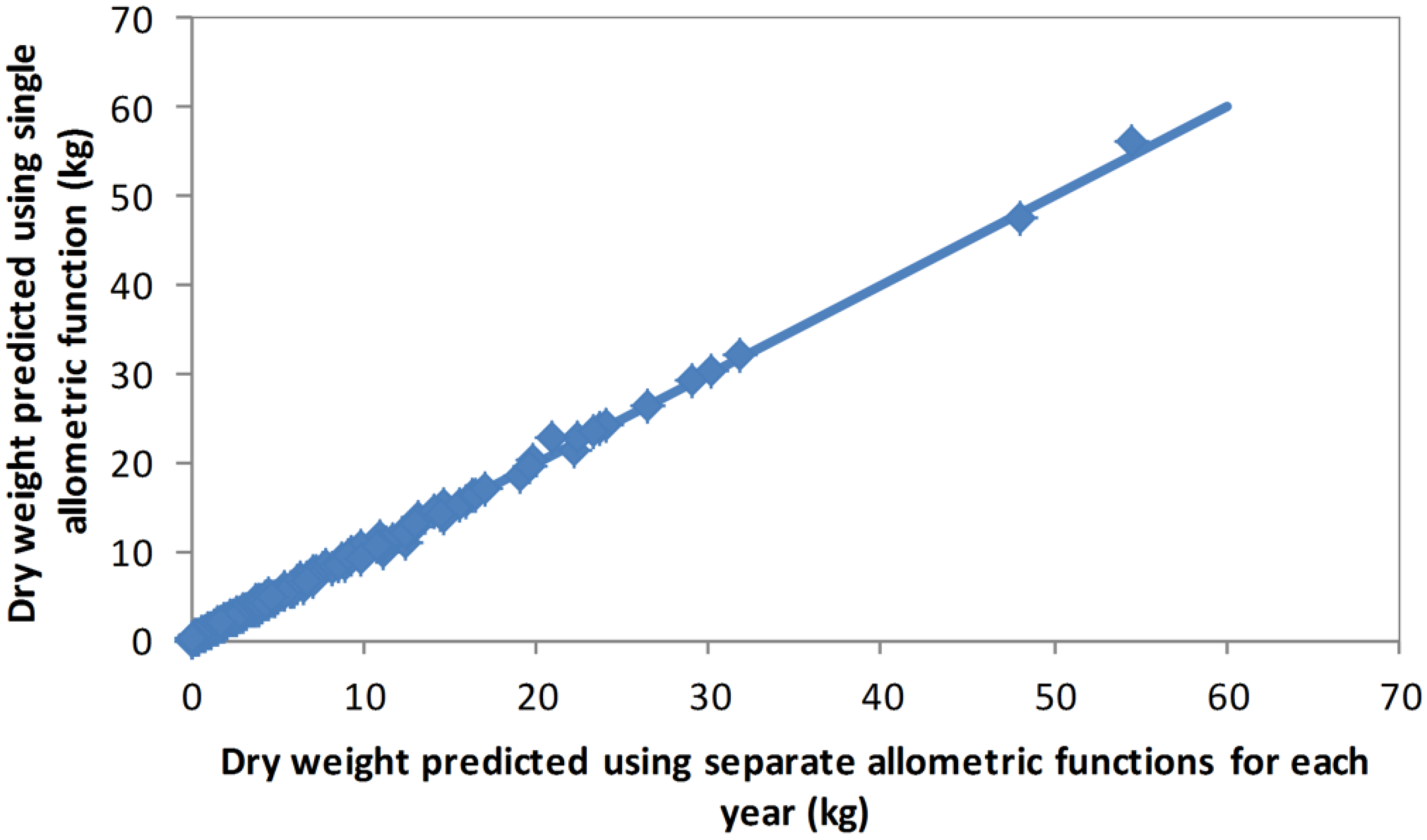
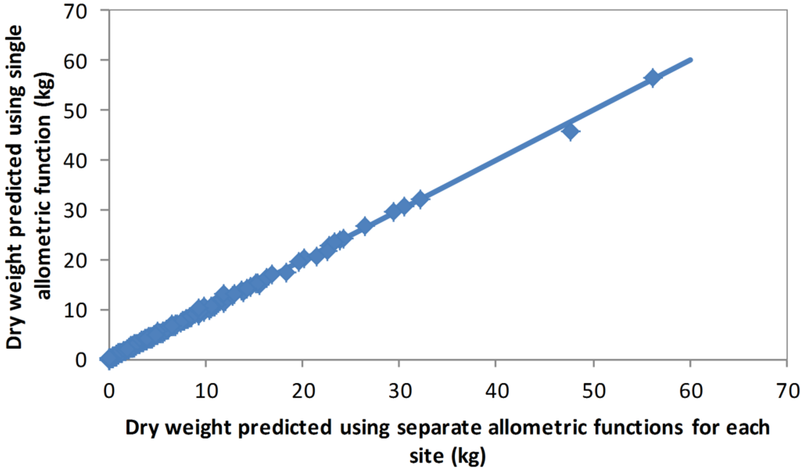
Separate models were fitted to the 2008 and 2012 biomass measurements to provide the best possible independent estimates of actual dry weight for each inventory (Table 2). However, for the backcast estimates, the 2012 allometric model was used as this method was intended to be based only on data collected in 2012. To test the sensitivity of the allometric model between years and across sites, predictions from the combined model were compared with predictions based on functions fitted separately for each year (2008 and 2012) and for each site (Oxford and d’Urville). These comparisons showed that differences in the allometric relationship between years and/or sites were negligible (Figure 1 and Figure 2).

Figure 1. Oven dry weights of individual shrubs estimated using a single allometric function developed from the combined biomass data, and using allometric functions developed separately for the 2008 and 2012 biomass data.

Figure 1. Oven dry weights of individual shrubs estimated using a single allometric function developed from the combined biomass data, and using allometric functions developed separately for the 2008 and 2012 biomass data.

Figure 2. Oven dry weights of individual shrubs estimated using a single allometric function developed from the combined biomass data, and using allometric functions developed separately for the Oxford and d’Urville biomass data.

Figure 2. Oven dry weights of individual shrubs estimated using a single allometric function developed from the combined biomass data, and using allometric functions developed separately for the Oxford and d’Urville biomass data.

Estimated carbon stocks in 2008 and 2012 obtained by applying these allometric models to the inventory plot data are summarised in Table 3. Carbon stocks were higher at d’Urville, where above-ground biomass (AGB) carbon averaged 12.2 t/ha in 2008 and 20.9 t/ha in 2012, and the calculated increase in carbon stock was 8.7 t/ha, than at Oxford, where AGB carbon averaged 6.2 t/ha in 2008 and 10.7 t/ha in 2012, and the calculated increase in carbon was 4.5 t/ha. The actual time interval between measurements varied somewhat between plots and sites, and was less than five complete years. Stems that died over the interval between measurements comprised almost 13% of the biomass increment at d’Urville and 11% at Oxford. While still evident on the plot, none of the stems that were dead in 2008 were still standing when these plots were re-measured in 2012, owing to decay at ground level. The dead matter would have increased the size of the litter pool. However losses owing to decay were not considered.

Table 3. Estimated carbon stock (t/ha) of above-ground live biomass carbon in 2008 and 2012, increase in the pool over 2008–2012, and carbon stock of stems that died between 2008 and 2012. In plots where only a sample of stems was re-measured in 2012, estimates have been adjusted for missing stems using the basal area ratio method.

Site	Plot	Live 2008	Live 2012	Increase in Live 2008–2012	Stems Died 2008–2012
D’Urville	D3	10.2	21.5	11.4	0.0
	D4	36.3	56.2	19.9	3.1
	D5	3.1	5.7	2.6	0.1
	D7	13.8	22.8	9.0	0.0
	D8	3.5	6.8	3.3	1.2
	D9	6.3	13.9	7.5	4.1
	D10	24.3	36.4	12.1	3.0
	D11	3.9	9.9	6.0	1.3
	D12	20.7	35.1	14.4	0.0
	D13	0.1	1.1	1.1	0.8
	Average	12.2	20.9	8.7	1.4
	std. error	3.7	5.5	1.9	0.5
Oxford	C1	10.8	21.0	10.2	2.5
	C2	9.8	12.9	3.1	0.3
	C3	4.2	7.9	3.7	0.0
	C4	14.0	26.8	12.8	0.7
	C5	1.3	2.0	0.7	0.0
	C6	1.5	2.7	1.2	0.1
	C7	3.3	5.1	1.8	0.2
	C8	4.6	7.1	2.4	0.7
	Average	6.2	10.7	4.5	0.6
	std. error	1.7	3.2	1.6	0.3

Table 3. Estimated carbon stock (t/ha) of above-ground live biomass carbon in 2008 and 2012, increase in the pool over 2008–2012, and carbon stock of stems that died between 2008 and 2012. In plots where only a sample of stems was re-measured in 2012, estimates have been adjusted for missing stems using the basal area ratio method.

Site	Plot	Live 2008	Live 2012	Increase in Live 2008–2012	Stems Died 2008–2012
D’Urville	D3	10.2	21.5	11.4	0.0
	D4	36.3	56.2	19.9	3.1
	D5	3.1	5.7	2.6	0.1
	D7	13.8	22.8	9.0	0.0
	D8	3.5	6.8	3.3	1.2
	D9	6.3	13.9	7.5	4.1
	D10	24.3	36.4	12.1	3.0
	D11	3.9	9.9	6.0	1.3
	D12	20.7	35.1	14.4	0.0
	D13	0.1	1.1	1.1	0.8
	Average	12.2	20.9	8.7	1.4
	std. error	3.7	5.5	1.9	0.5
Oxford	C1	10.8	21.0	10.2	2.5
	C2	9.8	12.9	3.1	0.3
	C3	4.2	7.9	3.7	0.0
	C4	14.0	26.8	12.8	0.7
	C5	1.3	2.0	0.7	0.0
	C6	1.5	2.7	1.2	0.1
	C7	3.3	5.1	1.8	0.2
	C8	4.6	7.1	2.4	0.7
	Average	6.2	10.7	4.5	0.6
	std. error	1.7	3.2	1.6	0.3

The test data were acquired to assess the reliability of backcasting growth in live stems from a single inventory measurement in 2012. This analysis was therefore restricted to live stems with a basal diameter measurement and a height measurement at both measurement dates. Restricting the analysis in this way allowed a direct comparison between measured and predicted basal areas and heights. Consequently, the resultant dry weight stock and stock change estimates of this analysis differ somewhat from those presented in Table 3. Across both sites, 82% (302) of the live plants re-identified in 2012 were measured for height and diameter in both 2008 and 2012.

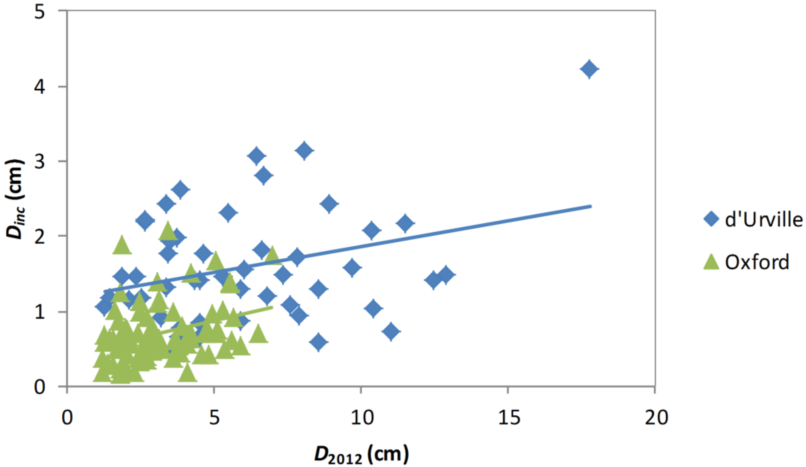
Stem analysis data revealed a positive relationship between D_inc and D₂₀₁₂ with growth rates greater at d’Urville than Oxford (Figure 3). 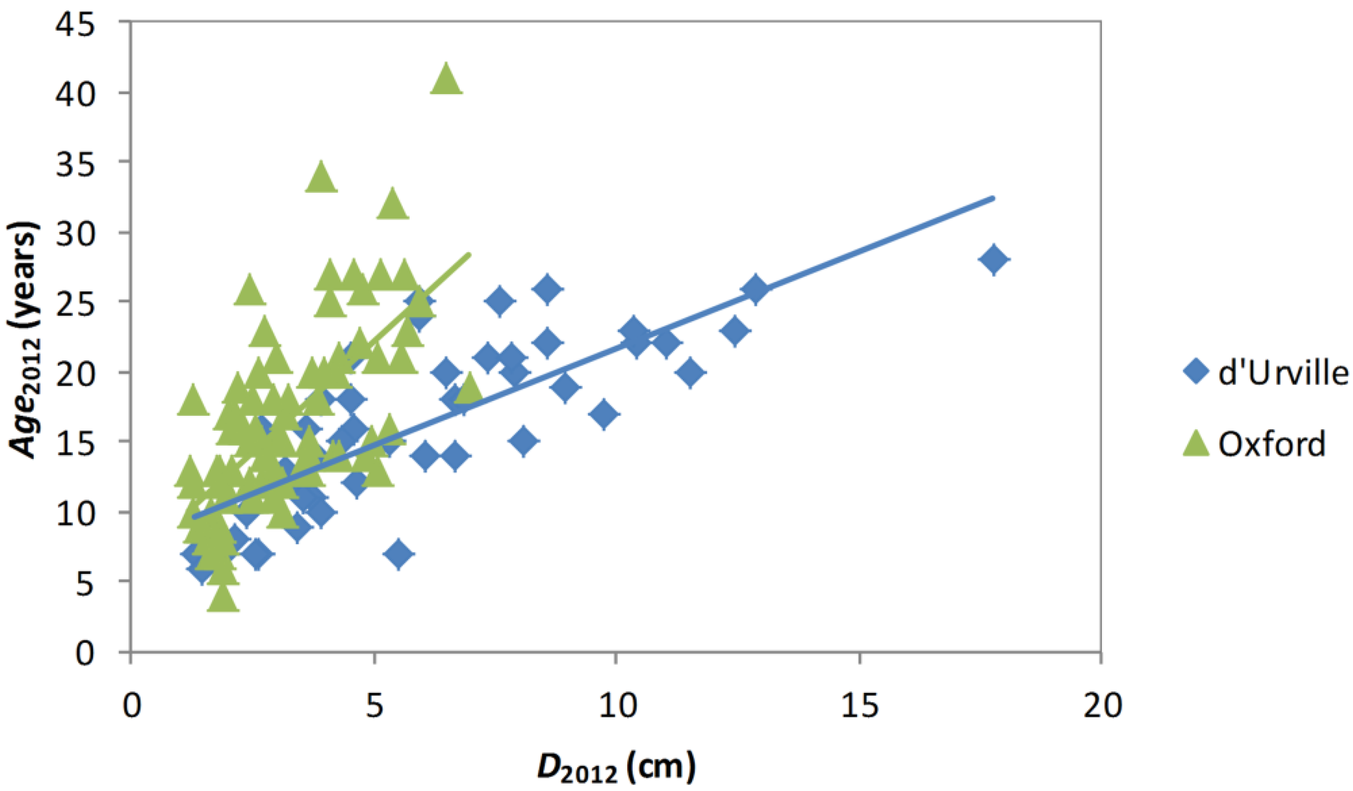When the model for predicting D_inc from D₂₀₁₂ was fitted to the diameter increment disc data (Equation (2), n = 130, R² = 0.78), the slope of the relationship varied significantly between plots (F_17,87 = 3.51, p < 0.0001), but species effects were not significant (F_7,87 = 2.10, p = 0.052). As expected, there was a positive relationship between stem age in 2012 and diameter, with the relationship varying between sites (Figure 4). When Equation (3) was fitted (n = 130, R² = 0.74), the slope of the relationship differed significantly between plots (F_17,87 = 3.03, p < 0.0001), but species effects were not significant (F_7,87 = 1.78, p = 0.16).

When testing the backcasting procedure, the species terms in Equations (2) and (3) were retained even though they were not statistically significant. This was done to maintain generality in the testing procedure as it might be expected that species differences in growth rates would be more apparent in larger-scale inventories. In practice, backcast estimates of carbon in this pilot study obtained using models with and without species effects were similar.

Figure 3. Relationships between D_inc and D₂₀₁₂ for d’Urville and Oxford. Lines show linear regressions for each site.

Figure 3. Relationships between D_inc and D₂₀₁₂ for d’Urville and Oxford. Lines show linear regressions for each site.

Figure 4. Relationships between Age₂₀₁₂ and D₂₀₁₂ for d’Urville and Oxford. Lines show linear regressions for each site.

Figure 4. Relationships between Age₂₀₁₂ and D₂₀₁₂ for d’Urville and Oxford. Lines show linear regressions for each site.

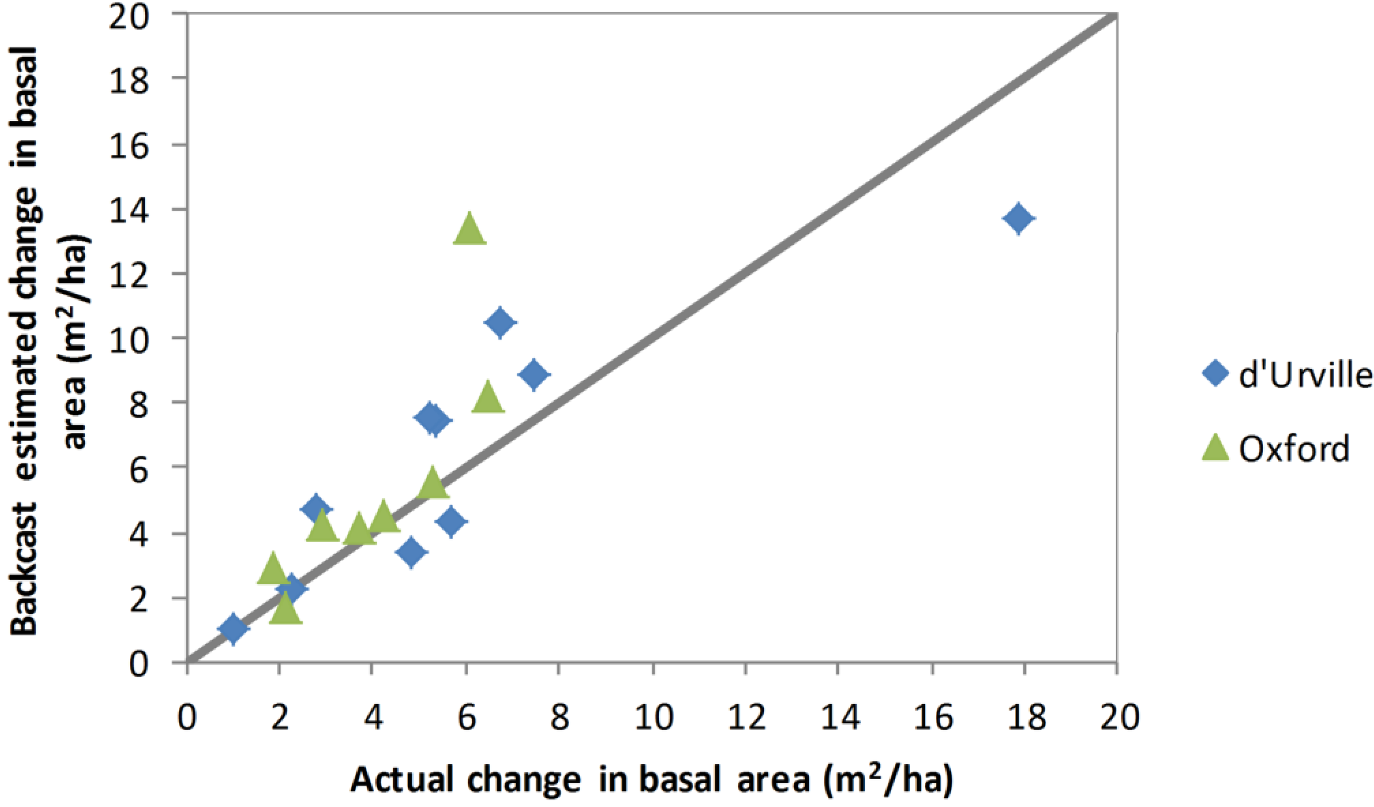
The results of estimating change in basal area of live stems from 2008 to 2012 from the 2012 inventory using diameter growth rates based on the basal disc analysis (the backcast method) are compared with the actual change in basal area in Figure 5. Although there were some outliers, the backcast estimate of change in basal area was in reasonably close agreement with actual change in basal area for both sites.

Figure 5. Backcast estimated 2008–2012 change in basal area versus actual change in basal area for plants measured for diameter and height in both 2008 and 2012. Values shown are plot means. The line indicates the y = x relationship.

Figure 5. Backcast estimated 2008–2012 change in basal area versus actual change in basal area for plants measured for diameter and height in both 2008 and 2012. Values shown are plot means. The line indicates the y = x relationship.

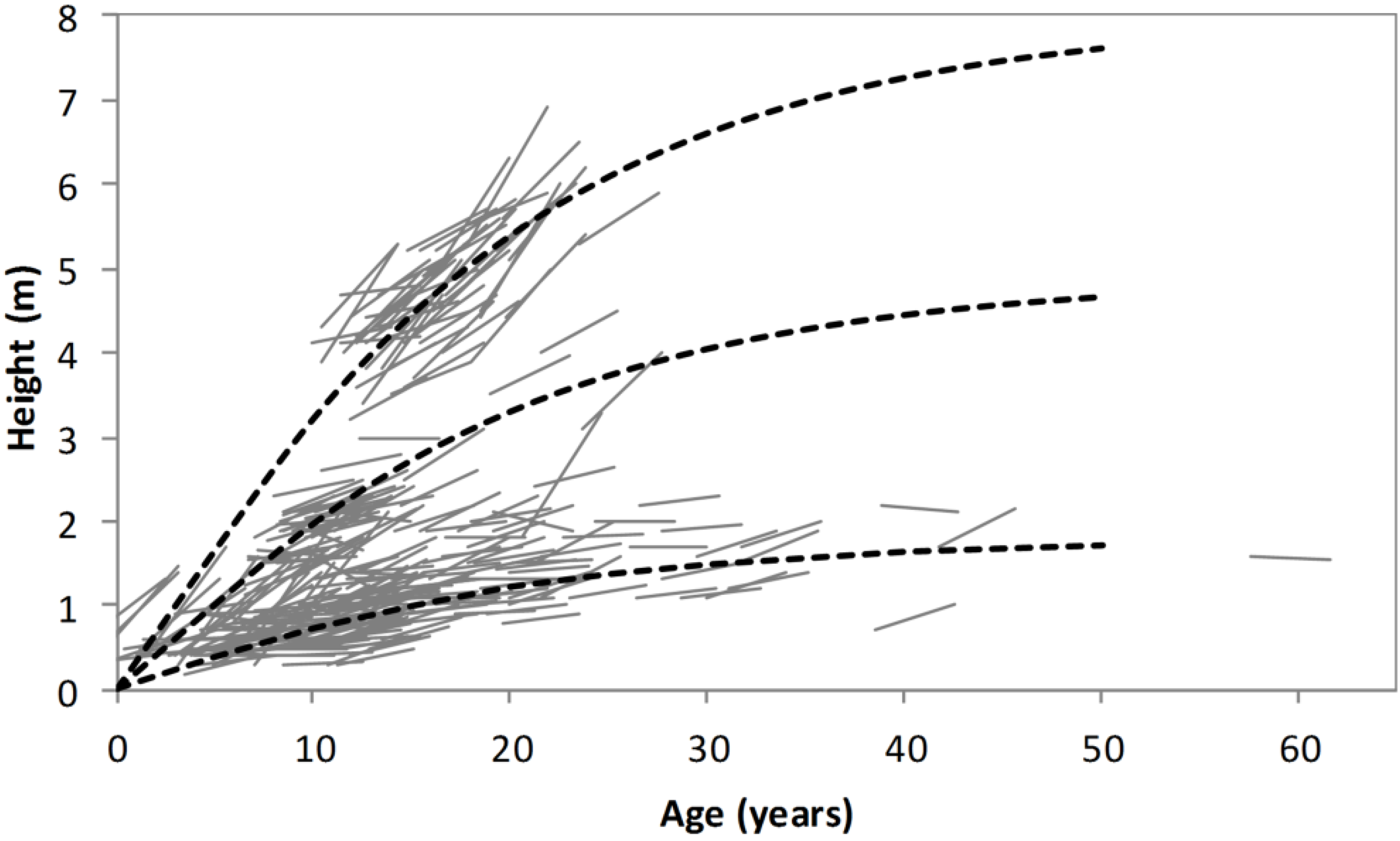
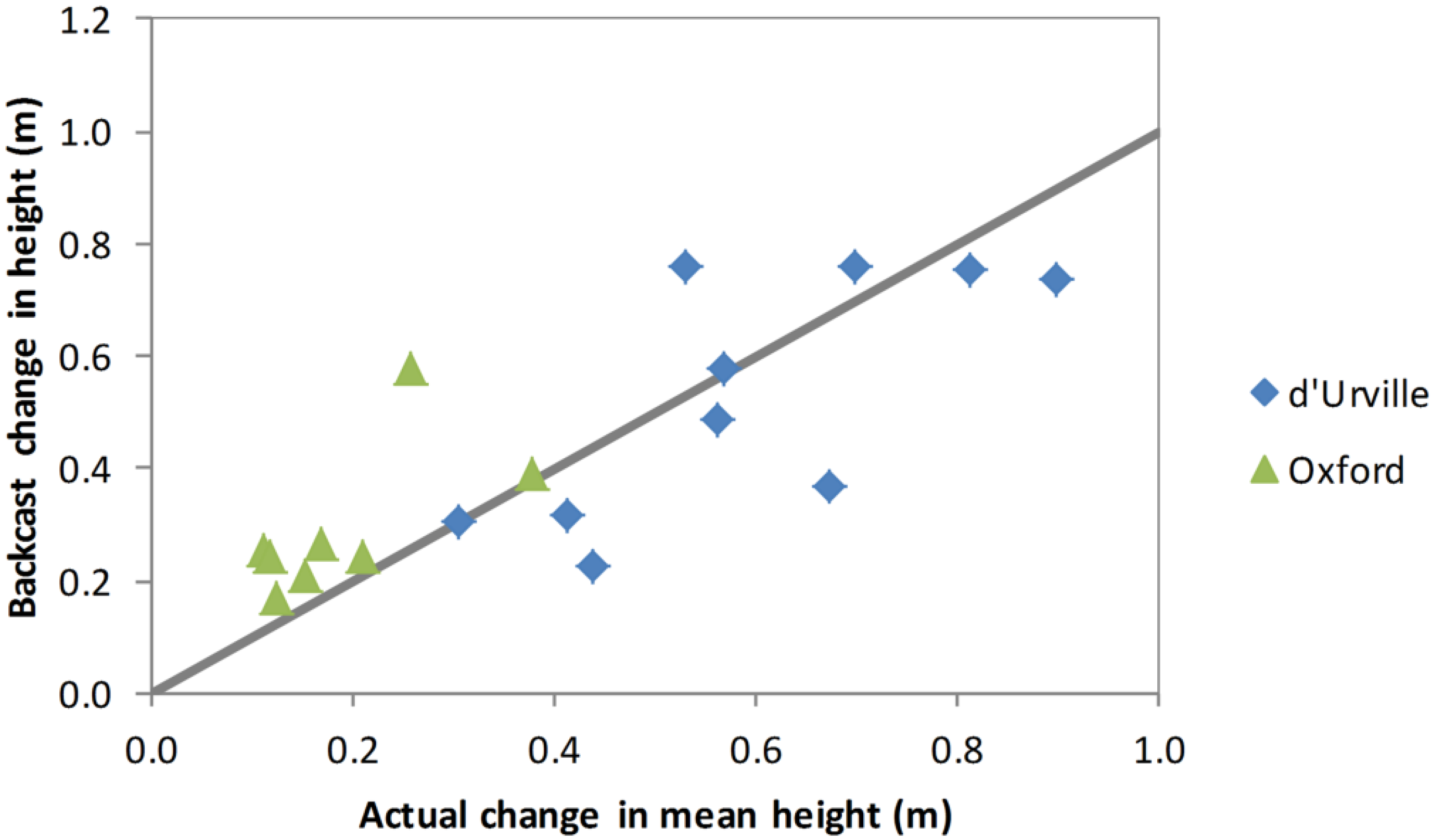
The method of backcasting shrub height is illustrated in Figure 6. Firstly, the age of each stem was estimated using Equation (3). Then, a generic height/age function (Equation (4)) was used to backcast the height of each stem the required number of years. The generic height/age function forms a family of anamorphic growth curves which are scaled for each stem to agree with height as measured in 2012. This backcasting procedure for shrub height accurately predicted the 2008–2012 change in height for d’Urville but slightly overestimated it for Oxford (Figure 7).

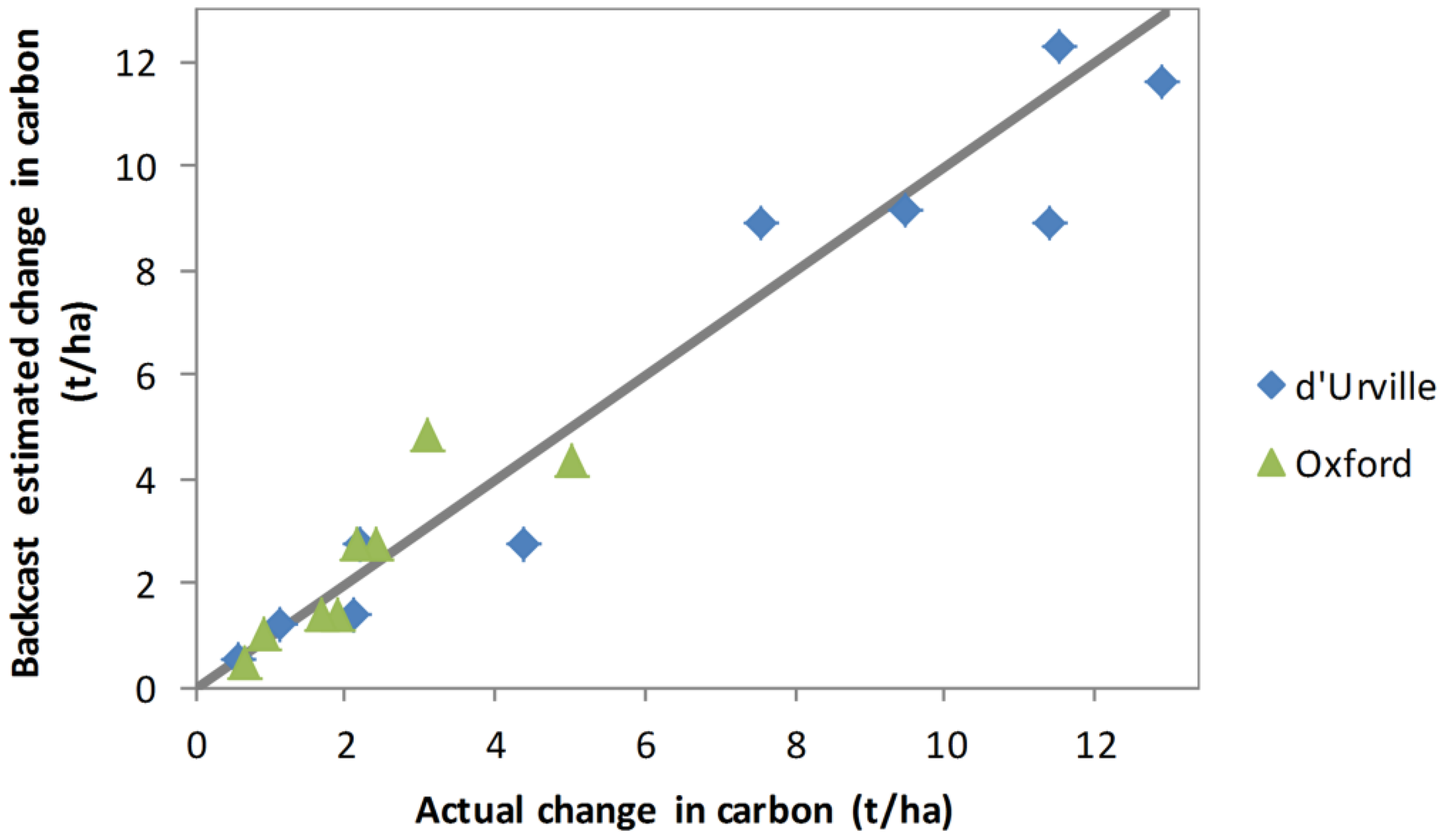
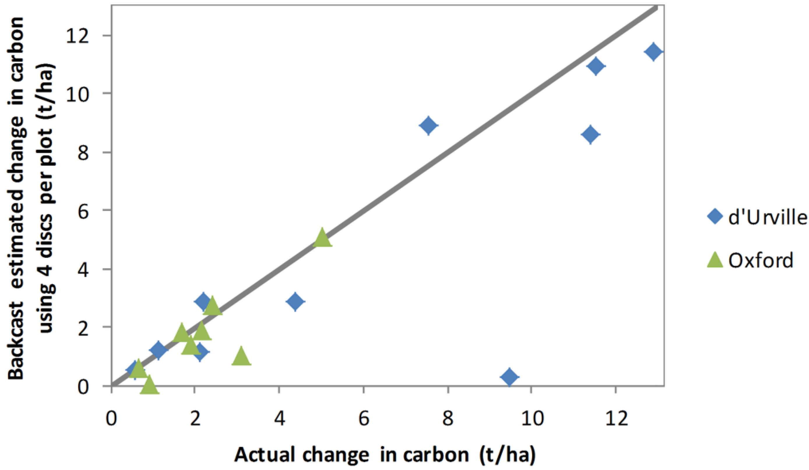
The results of estimating 2008–2012 carbon sequestration by applying the 2012 allometric model to the 2008 backcast estimates of basal area and height are compared with actual estimates in Table 4 and Figure 8. Backcast estimates of carbon sequestration were generally very satisfactory. Using this method, the estimated increase in live biomass carbon for d’Urville was 6.0 t/ha compared with an actual increase for the same plants based on the independent 2008 and 2012 inventories of 6.3 t/ha. At Oxford the estimated increase was 2.4 t/ha compared with an actual increase of 2.2 t/ha. The standard error of the backcast increase in live biomass carbon was similar to the standard error of the directly measured increase in carbon.

On average, 7.3 basal discs were sampled per plot, with numbers ranging between 4 and 14. To test whether the backcasting method was sensitive to the number of basal discs sampled, Equations (2) and (3) were refitted using only the 4 basal discs per plot from biomass samples. Backcast carbon sequestration estimates obtained using these equations are compared with actual sequestration (Figure 9). Although estimates for most plots were similar to those obtained using all discs (Figure 8), estimates for several plots were quite poor.

Figure 6. Illustration of the procedure used for backcasting height. The dashed lines show the family of height/age functions described by Equation (4) for low, medium and fast growing shrubs. The solid lines show 2008–2012 heights of measured stems, with ages estimated using Equation (3).

Figure 6. Illustration of the procedure used for backcasting height. The dashed lines show the family of height/age functions described by Equation (4) for low, medium and fast growing shrubs. The solid lines show 2008–2012 heights of measured stems, with ages estimated using Equation (3).

Figure 7. Backcast estimated 200–2012 change in height versus actual change in height for plants measured for diameter and height in both 2008 and 2012. Values shown are plot means. The line indicates the y = x relationship.

Figure 7. Backcast estimated 200–2012 change in height versus actual change in height for plants measured for diameter and height in both 2008 and 2012. Values shown are plot means. The line indicates the y = x relationship.

4. Discussion

4.1. Prediction of Stock Changes in 2008 by Backcasting from 2012 Inventory Data

Because no inventory of New Zealand’s post-1989 natural forest was performed in 2008, carbon stock changes since 2008 will need to be modelled from shrub basal diameter and height measurements made in 2012, supplemented with growth measurements and ring counts from basal disc samples. This pilot study showed that modelled above-ground live biomass carbon stocks in 2008 were comparable in accuracy and precision to directly measured estimates. Basal disc samples provide estimates of stem diameter increment annually and of plant age from ring counts, with the latter utilized in height/age functions, calibrated using field plot measurements of height in 2012, to estimate height in 2008. After taking species and age into account, predictions of carbon sequestration in live plants in field plots, derived by backcasting basal area and height from the 2012 measurement, were comparable in accuracy and precision to estimates obtained directly by re-measuring the plots.

Figure 8. Backcast estimated 2008–2012 change in carbon versus actual change in carbon for plants measured for diameter and height in both 2008 and 2012. Values shown are plot means. The line indicates the y = x relationship.

Figure 8. Backcast estimated 2008–2012 change in carbon versus actual change in carbon for plants measured for diameter and height in both 2008 and 2012. Values shown are plot means. The line indicates the y = x relationship.

Figure 9. Backcast estimated 2008–2012 change in carbon using 4 discs per plot versus actual change in carbon. Values shown are plot means. The line indicates the y = x relationship.

Figure 9. Backcast estimated 2008–2012 change in carbon using 4 discs per plot versus actual change in carbon. Values shown are plot means. The line indicates the y = x relationship.

Table 4. Estimated carbon stock (t/ha) of above-ground live biomass carbon in 2012, 2008, and backcast estimates for 2008, along with actual and backcast estimates of carbon change between 2008 and 2012. Values are for plants measured for diameter and height in both 2008 and 2012.

Site	Plot	2012	2008	Backcast 2008	Actual Increase 2008–2012	Backcast Increase 2008–2012
D’Urville	D3	21.5	10.2	12.7	11.4	8.9
	D4	27.1	17.7	18.0	9.5	9.1
	D5	4.9	2.8	3.5	2.1	1.4
	D7	20.5	12.9	11.6	7.5	8.9
	D8	2.9	1.8	1.7	1.1	1.2
	D9	5.7	3.5	3.0	2.2	2.8
	D10	34.6	23.1	22.3	11.5	12.3
	D11	8.1	3.7	5.4	4.4	2.8
	D12	31.5	18.7	20.0	12.9	11.6
	D13	0.6	0.1	0.1	0.6	0.6
	Average	15.8	9.4	9.8	6.3	6.0
	std. error	4.0	2.6	2.6	1.5	1.5
Oxford	C1	5.6	3.2	2.9	2.4	2.8
	C2	13.0	9.9	8.2	3.1	4.9
	C3	4.2	2.3	2.8	1.9	1.4
	C4	13.8	8.8	9.4	5.0	4.3
	C5	2.0	1.3	1.5	0.7	0.5
	C6	2.2	1.3	1.2	0.9	1.0
	C7	4.7	3.0	3.3	1.7	1.4
	C8	6.3	4.1	3.5	2.1	2.8
	Average	6.5	4.2	4.1	2.2	2.4
	std. error	1.6	1.2	1.1	0.5	0.6

Table 4. Estimated carbon stock (t/ha) of above-ground live biomass carbon in 2012, 2008, and backcast estimates for 2008, along with actual and backcast estimates of carbon change between 2008 and 2012. Values are for plants measured for diameter and height in both 2008 and 2012.

Site	Plot	2012	2008	Backcast 2008	Actual Increase 2008–2012	Backcast Increase 2008–2012
D’Urville	D3	21.5	10.2	12.7	11.4	8.9
	D4	27.1	17.7	18.0	9.5	9.1
	D5	4.9	2.8	3.5	2.1	1.4
	D7	20.5	12.9	11.6	7.5	8.9
	D8	2.9	1.8	1.7	1.1	1.2
	D9	5.7	3.5	3.0	2.2	2.8
	D10	34.6	23.1	22.3	11.5	12.3
	D11	8.1	3.7	5.4	4.4	2.8
	D12	31.5	18.7	20.0	12.9	11.6
	D13	0.6	0.1	0.1	0.6	0.6
	Average	15.8	9.4	9.8	6.3	6.0
	std. error	4.0	2.6	2.6	1.5	1.5
Oxford	C1	5.6	3.2	2.9	2.4	2.8
	C2	13.0	9.9	8.2	3.1	4.9
	C3	4.2	2.3	2.8	1.9	1.4
	C4	13.8	8.8	9.4	5.0	4.3
	C5	2.0	1.3	1.5	0.7	0.5
	C6	2.2	1.3	1.2	0.9	1.0
	C7	4.7	3.0	3.3	1.7	1.4
	C8	6.3	4.1	3.5	2.1	2.8
	Average	6.5	4.2	4.1	2.2	2.4
	std. error	1.6	1.2	1.1	0.5	0.6

The change in the litter carbon pool from plants that died between 2008 and 2012 was small relative to the change in the above-ground live biomass pool over this period, with the litter contribution averaging 11% at d’Urville and 7% at Oxford of the carbon stock change in live plants. Stems that died had fallen over within 5 years, so the contribution to the total carbon stock from litter could be modelled using decay functions and by making assumptions about the mortality date. Otherwise its contribution will be overestimated. Root biomass carbon has proved to be difficult to measure in naturally regenerating manuka/kanuka shrubland in New Zealand. Root/shoot ratios reportedly averaged approximately 0.15–0.2 [11,12], although the estimate of 0.15 was considered to be an underestimate. An average root/shoot ratio of 0.20 appears to be more reasonable for manuka and kanuka. More research on root/shoot ratios of arboreal shrubs in secondary forest is warranted.

4.2. Data Quality

The use of callipers to measure annual growth rings in the laboratory provided more accurate increment data than generally obtainable from repeated measurements of basal diameters in the field, because it was possible to take into consideration the non-circular nature of individual rings. For example, inner growth rings were often circular, while basal discs became increasingly elliptical due to asymmetric growth of outer rings. Two orthogonal diameter measurements (one being the maximum diameter) were therefore made for each growth ring. Further, the height above-ground at which diameters were measured was invariably the same when measuring basal disc samples in the laboratory. This was rarely possible in field plots assessed in 2008 and 2012 because in most cases the measurement point was not permanently marked. Nevertheless, when determining stock changes, shrub basal diameter and height measurement errors comprised a relatively small proportion of the overall error in stock estimates, which were mostly related to shrub allometry [13].

False rings were evident in some species which can lead to errors in diameter increment and age determination using cores, which can be avoided using basal disc samples. Growth rings needed to be continuous around the circumference of the disc to be able to distinguish false rings from true annual rings, and hence obtain an accurate estimate of shrub age and measurements of diameter increment. Some staining of growth rings was apparent, especially if disc samples had not been frozen while in storage, which made identification of annual rings more difficult. In a few instances a basal disc was hollow due to internal decay and diameter increment and age had to be extrapolated from increment trend evident in outer growth rings.

4.3. Considerations Regarding Post-1989 Natural Forest Inventory Plots

It proved time consuming to measure the basal diameter and height of individual shrubs in a 5 × 5 m subplot, so the methodology to be applied in national inventory plots could be modified. It is suggested that 4 small circular subplots be installed, one in the centre of each quadrant of the 20 × 20 m plot. A radius of 1.5 m would be practical, and four subplots will give a total assessment area of 28.27 m², which is slightly greater than for one 5 × 5 m subplot as used in the pilot study.

It will be necessary to cut basal disc samples from plants outside of the 20 × 20 m plot to develop relationships between diameter increment and basal diameter. We recommend that discs from 2 shrubs representing plants growing in each of the 1.5 m radius subplots (8 discs per plot) would be sufficient. In the pilot study, good estimates were obtained using an average of 7.3 discs per plot. In fact, good estimates were usually obtained using only 4 discs per plot, although this sample number produced poor estimates for several plots (Figure 9). We further recommend that biomass measurements be undertaken for half of the felled plants, because allometry is an important source of the overall field measurement/model estimation error [13]. More than four biomass plants per plot would seem to be unnecessary, based on the results from the pilot study. We feel that biomass sampling is necessary to cover species adequately, because differences in allometry may occur across the wide range of sites likely to be encountered in a national sample. The methods developed for post-1989 natural forest plots could potentially be used to estimate carbon stocks and changes in pre-1990 natural forest plots more precisely than is currently possible from dbh measurements. Stem dbh re-measurement errors can be significant in large trees. In contrast, precise measurements of stem diameter increment would be possible using breast height core samples from plot trees selected by species and size classes. In practice, this methodology could be difficult to implement for several reasons. For example, pith-to-bark core sampling, to determine tree age and growth rate, is not possible if trees are hollow and may not be feasible if trees are very large. Furthermore, dead organic matter pools can be substantial in mature forest ecosystems, and periodic assessments of tree status (live or dead) provides information on the year of mortality that allows carbon stocks and changes in dead wood to be modeled using decay functions [14]. For these reasons, periodic re-measurement of plots will be necessary when inventorying carbon stocks in pre-1990 forest.

5. Conclusions

• The plot measurement and biomass sampling procedures at Oxford and d’Urville allowed live biomass stocks to be estimated in 2008 and 2012. The measured stock changes were similar to stock changes predicted, using backcasting methods, from stem analysis of basal disc samples from representative shrubs growing adjacent to each plot.
• Above-ground live biomass comprised the majority of carbon stock in the pilot study, and these plots are likely to be representative of plots in New Zealand’s post-1989 natural forest. Nevertheless, in an inventory of post-1989 natural forest it will be important to measure the diameter and height of dead stems, and predict losses owing to decay.
• General allometric models could be applied to plot data to estimate carbon in individual shrubs and small trees, and while manuka and kanuka are likely to dominate, there is uncertainty around which species will be encountered and what growth rates will be found in national inventory plots, and therefore biomass and supplementary disc sampling will be necessary.
• The diameter, height, and decay class of dead stems, and assumptions around the stem mortality rate will allow carbon stocks and changes to be estimated for the dead wood and litter pools. However, dead organic matter is expected to comprise a small proportion of the total carbon stock (excluding soil C).